3. Load Analysis and Forecasting
1
Highlights
Ameren Missouri expects energy consumption to grow 23% and peak demand to grow 18% over the next 20 years.
The commercial class is expected to provide the most growth while federal efficiency standards slow residential growth compared to historical trends. The estimated range of peak demand uncertainty is 2,183 MW in 2030.
Key forecast uncertainties include growth in miscellaneous plug load, the adoption of electric vehicles, and the impact of rising prices.
Significant enhancements have been made throughout the forecasting process to include more end-use detail.
Ameren Missouri has developed a range of load forecasts consistent with the scenarios outlined in Chapter 2. These load forecasts provide the basis for estimating Ameren Missouri‟s future resource needs and provide hourly load information used in the modeling and analysis discussed in Chapter 9. In addition, the Statistically Adjusted End-use forecasting tools and methods End-used to the develop the forecasts provided a solid analytical basis for testing and refining the assumptions used in the development of the potential demand-side resource portfolios discussed in Chapter 7. The energy intensity of the future economy and the inherent energy efficiency of the stock of energy using goods are explored throughout the analysis to arrive at reasonable estimates of high, base, and low load growth.
3.1 Energy Forecast
This chapter describes the forecast of Ameren Missouri‟s energy, peak demand, and customers that underlies the analysis of resources undertaken in this IRP. In order to account for a number of combinations of possible economic and policy outcomes, ten different forecasts were prepared. Based on the subjective probabilities of these scenarios identified by Ameren Missouri, an eleventh case was developed to represent the base, or planning case for the study. The planning case forecast projects Ameren Missouri‟s retail sales to grow by 1.09% annually between 2010 and 2030, and retail peak demand to grow by 0.91% per year.
1 4 CSR 240-22.030(8)(H)
As with any forecast of energy, there are several underlying assumptions. Expectations for economic growth underlying the load forecast are from Moody‟s Analytics‟ (formerly Economy.com) forecast of economic conditions in the Ameren Missouri service territory. Expectations about future energy market conditions, such as fuel prices and the impact on electricity prices of different environmental policy regimes are based on modeling results from Charles River Associates (CRA) and their interviews with internal Ameren subject matter experts.
Compared to Ameren Missouri‟s last IRP, filed in 2008, both the level and the growth rate of the forecast are lower. In the 2008 IRP, the 2010 sales were expected to be 39,623 GWh, as compared to an expectation at the time of forecast in this IRP of 38,110 GWh. The initial level of sales is lower primarily because the unusually severe recession that Missouri and the US experienced between 2007 and 2009, and the impact that has had on energy consumption. The 1.09% growth rate in retail sales for the 2010-2030 time period in this filing is also lower than the 1.48% retail sales growth rate expected for the same time period in the 2008 IRP forecast largely due to the effects of energy efficiency codes and standards, many of which were established as a part of the Energy and Information Security Act of 2007 (EISA 2007) after the 2008 IRP forecast had been prepared. Finally, expectations of higher energy prices than were contemplated in the 2008 filing also slow the rate of growth through assumed customer conservation efforts. It should be noted that in the development of this forecast, only the underlying growth of energy efficiency due to market conditions was included. The energy efficiency impacts of Ameren Missouri‟s energy efficiency and demand side management (DSM) programs
were calculated in a separate and parallel process and then added to forecast results. So the energy efficiency changes embedded in the energy forecasts presented in this section of the IRP are only the result of changes other than Ameren Missouri‟s specific programs, such as changes to Federal law, or changes in consumer behavior. The impacts of Ameren Missouri‟s measureable DSM and energy efficiency programs are included in the
IRP and thus affect the choice of the optimal supply side plan, but were not part of the load forecast process. For that reason Ameren Missouri‟s DSM and energy efficiency programs are not discussed in forecasting section of the IRP documentation. They are discussed in great detail in Chapter 7.
The modeling of carbon policy and the other critical dependent uncertain factors is another key difference between this IRP and the 2008 IRP. For this IRP, ten scenario forecasts were produced based on different assumptions about the future path of load growth, natural gas prices, and carbon policy. Those scenarios and their development are discussed in more detail in section 3.1.5.
3.1.1 Historical Database
Ameren Missouri tracks its historical sales and customer counts2 by revenue class
(Residential, Commercial, and Industrial)3, and also by rate class (Small General Service,
Large General Service, Small Primary Service, and Large Primary Service). Ameren Missouri uses these rate classes as the sub-classes for forecasting, both because the data is readily accessible from the billing system and because it provides relatively homogeneous groups of customers in terms of size4. Historical billed sales are available
for all rate and revenue classes back to January 19955. At the time of the preparation of
the load forecast for this IRP, historical sales were known through December of 2009. Except as noted later in this document, any data presented for 2010 or beyond is forecasted data and data from 2009 and earlier is actual metered sales data. Historical energy consumption and customer count data is available in the Appendix to Chapter 36. Ameren Missouri routinely weather normalizes the observed energy consumption of its customers to remove the impact of unusual weather patterns. The process for weather normalizing sales is described in section 3.3, and weather normalized historical consumption from 1995 forward is also reported in the Appendix7. In Ameren Missouri‟s
2008 IRP, the historical sales for the wholesale class were normalized to remove the load associated with expired contacts. The load data in this IRP starts with that historical data set and reports sales from that point forward based on the mix of wholesale customers that existed at the time.
The appendix includes use per unit energy sales and demand data for all classes8. In each case, the unit included in the analysis is the customer count for the class. This is selected because it is a measured value for each class that is accessible and meaningful in all cases9.
3.1.2 Service Territory Economy
The Ameren Missouri electric service territory is comprised of 59 counties in eastern and central Missouri (It should be noted, however, that although Ameren Missouri serves customers in 59 counties, it does necessarily not serve every electric customer in those counties). As would be expected, the level of sales is highly correlated with the behavior of the economy in the service territory.
2 4 CSR 240-22.030(1)(B)1 3 4 CSR 240-22.030(1)(A) 4 4 CSR 240-22.030(1)(A)1-2 5 4 CSR 240-22.030(1)(D), 4 CSR 240-22.030(1)(D)1 6 4 CSR 240-22.030(1)(B)1 7 4 CSR 240-22.030(1)(B)1 8 4 CSR 240-22.030(1)(C) 9 4 CSR 240-22.030(1)(C)1, 4 CSR 240-22.030(5)(B)2
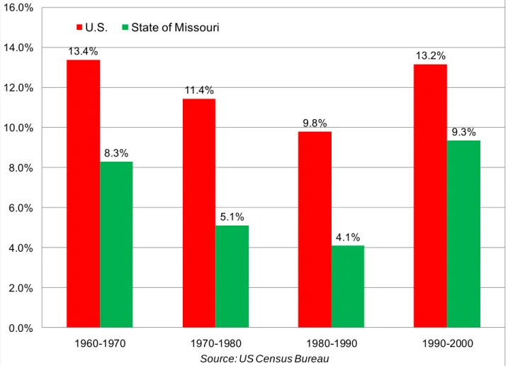
Figure 3.1: US and Missouri Population Change by Decade
Historically, the Ameren Missouri service territory has been characterized by slower demographic growth than the US as a whole. In that respect, the service territory‟s
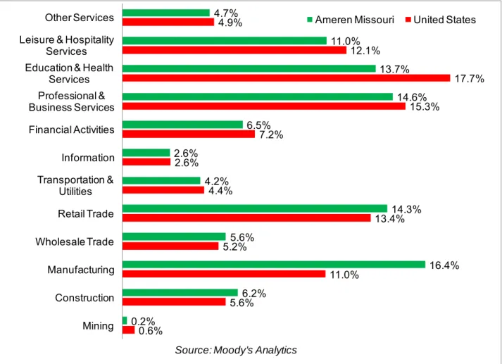
economy is not terribly different from most other Midwestern states and metropolitan areas. Like much of the Midwest, the region‟s economy was based on manufacturing for many years, but over the past several decades the share of the territory‟s employment in manufacturing has been declining while employment in services, particularly health care, has grown. So although the service territory still has a higher than average share of employment in manufacturing, it is no longer the employment growth engine it once was. The allocation of service territory employment by NAICS sector is shown in Figure 3.2; a list of some of the largest employers in the service territory is in Table 3.1.
13.4% 11.4% 9.8% 13.2% 8.3% 5.1% 4.1% 9.3% 0.0% 2.0% 4.0% 6.0% 8.0% 10.0% 12.0% 14.0% 16.0% 1960-1970 1970-1980 1980-1990 1990-2000
U.S. State of Missouri
Figure 3.1: US and Ameren Missouri Service Territory Employment by Industry
The territory‟s major employers are spread across a number of different industries, but the region‟s single biggest employer is a hospital system, BJC Healthcare. Two other healthcare systems and three universities are among the largest employers in the territory, highlighting the importance of the health and education services to both the growth and level of employment, as well as to electricity sales.
As noted above, the service territory economy has grown at a slightly slower pace than the US as a whole because of slower demographic growth. In addition to the trend of slower demographic growth, the St. Louis region did not experience as big of a boost from the housing bubble as some other markets did.
The service territory economy also contains a number of nationally know financial firms, including Stifel Financial, Scottrade, and Edward Jones. These firms, however, were not among those that garnered headlines during the financial crisis in 2008.
0.6% 5.6% 11.0% 5.2% 13.4% 4.4% 2.6% 7.2% 15.3% 17.7% 12.1% 4.9% 0.2% 6.2% 16.4% 5.6% 14.3% 4.2% 2.6% 6.5% 14.6% 13.7% 11.0% 4.7% Mining Construction Manufacturing Wholesale Trade Retail Trade Transportation & Utilities Information Financial Activities Professional & Business Services Education & Health
Services Leisure & Hospitality
Services
Other Services Ameren Missouri United States
Table 3.1: Major Employers in the Ameren Missouri Service Territory
Figure 3.3: US and Ameren Missouri Households
Going forward Ameren Missouri expects that the service territory economy will recover apace with the US economy. Moody‟s Analytics predicts, and Ameren Missouri concurs, that the number of households will grow at an accelerating pace in 2011 and 2012 before slowing in the longer term. The acceleration in 2011 and 2012 is a rebound from 2009-2010, when weak housing and labor markets slowed household formation to a below
Employer Industry Number of Employees
BJC Healthcare Education & Health 23,378 Boeing Integrated Defense Systems Manufacturing 16,600 Wal- Mart Stores, Inc Retail Trade 13,400 Washington University Education & Health 12,390 SSM Health Care System Education & Health 12,102 Schnuck’s Markets Retail Trade 11,000 AT & T Incorporated Information 8,990 St. John’s Mercy Health Care Education & Health 8,876 University of Missouri Columbia Education & Health 8,188 Saint Louis University Education & Health 8,016 McDonald’s Leisure & Hospitality 8,000 AB InBev Manufacturing 6,000 Dierberg’s Markets Retail Trade 5,000 Edward Jones Financial Activities 4,422
Source: Moody’s Analytics
0 20 40 60 80 100 120 140 160 1990 1995 2000 2005 2010 2015 2020 2025 2030 S c a le d H o u s e h o ld s ( 1 9 9 0 = 1 0 0 ) Ameren Missouri United States
trend rate; as labor markets recover and home prices remain low household formation should increase at an above trend rate for a time. In both the short and the longer term, however, the number of households in the Ameren Missouri service territory will likely grow at a slower rate than in the US as a whole.
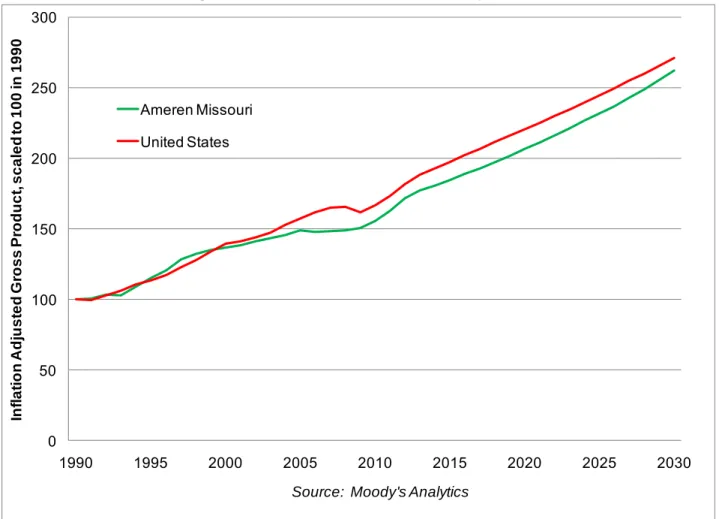
Figure 3.4: US and Service Territory GDP
Commercial sales are expected to be boosted by increased household formation and the attending demand for retail services as well the fact that the region‟s major employers in healthcare, education, and financial services are billed in our commercial class.
Long term risks to the service territory economic outlook include further declines in manufacturing such as the closure of the GM plant in Wentzville or the end of fighter aircraft production at Boeing. Upside risks would include faster population growth due to the area‟s low cost of living, faster than expected growth in the life sciences and financial sectors in the region, or faster than expected growth of energy intensive commercial customers such as data centers.
0 50 100 150 200 250 300 1990 1995 2000 2005 2010 2015 2020 2025 2030 In fl a ti o n A d ju s te d G ro s s P ro d u c t, s c a le d t o 1 0 0 i n 1 9 9 0 Ameren Missouri United States
3.1.3 Economic Drivers
10Several specific economic indicators were used as independent variables (independent variables in the forecasting models are often referred to as “drivers”) in our energy forecasting process.
For the residential class income, population, and the number of households in the service territory were used as drivers. For forecasts of commercial class sales, service territory GDP disaggregated by major industry group (NAICS sector), such as financial activities, educational & health services or professional & business services depending upon which sector or combination of sectors best correlates with each rate class‟ sales were used11.
For the forecast of industrial class sales, manufacturing employment and GDP were used as drivers depending upon the rate class and scenario. Table 3.2 illustrates key drivers and their expected growth over the IRP horizon12.
Table 3.2: Growth Rates of Selected Economic Drivers
Noteworthy in the forecast is the robust growth in manufacturing GDP. Moody‟s
Analytics forecast is for manufacturing output to grow faster than output in the other sectors of the service territory economy, but for manufacturing employment to grow slower than employment in the other sectors. This implies that service territory manufacturing will become more productive with respect to labor over the IRP forecast horizon. That implication is an important risk factor to the energy forecast. If industrial energy sales are closely correlated with manufacturing employment, then they will decline. If sales are more closely correlated with output, then they will grow more rapidly. The preferred strategy would be to let the past be the prologue in determining which variable to use, but in the past few years (specifically the time frame over which the forecasting models are estimated), manufacturing employment and output declined together. Therefore the effect of the predicted divergence is difficult to model. One could make a case for either variable as a driver, but if productivity growth is due to the
10 4 CSR 240-22.030(2)(A) 11 4 CSR 240-22.030(2)(C) 12 4 CSR 240-22.030(5)(B)1.A
Economic Driver CAGR, 2010-2030
Real Personal Income 1.9%
Population 0.4% Households 0.5% GDP 2.6% Manufacuring GDP 3.5% Employment 0.6% Manufacturing Employment 0.1%
replacement of workers with electricity consuming capital equipment, than output may be a better predictor of industrial electricity sales. As discussed below, this uncertainty was used to help shape the high, base, and low load growth scenarios.
The uncertainty about industrial sales is not the only source of uncertainty related to the economic drivers. The growth in residential sales over the next several years is dependent upon growth in households and the growth in use per household. Obviously, then, unforeseen changes in the number of households would cause changes in the amount of residential electricity demand.
3.1.4 Energy Forecasting
13This forecast of Ameren Missouri energy sales was developed with traditional econometric forecasting techniques, as well as a functional form called Statistically Adjusted End-Use (SAE). In the SAE framework, variables of interest related to economic growth, the price of electricity, and energy efficiency and intensity of end-use appliances, are combined into a small number of independent variables, which are used to predict the dependent variable (typically energy sales or sales per customer by class). The SAE framework was used to forecast energy sales in our residential general service rate class, and for all four of our commercial rate classes.
Statistically Adjusted End-Use (SAE)14
The advantage of the SAE approach is that it combines the benefits of engineering models and econometric models. Engineering models, such as REEPS, COMMEND and INFORM, modeled energy sales with a bottom up approach by building up estimates of end use by appliance type, appliance penetration, and housing unit or business type. These models are good at forecasting energy because they can be used to estimate the effects of future changes in saturations or efficiency levels, even if the changes are not present in observable history. In a traditional econometric model, it can be difficult to model precisely how the changing appliance efficiency standards will affect sales if the standards have been unchanged during the estimation period.
Econometric models, however, are estimated rather than calibrated, and it is easier to detect and correct any systematic errors in the forecasting model. For that reason, a system that combines the bottom up approach of engineering models with an econometric approach should produce more accurate forecasts. The SAE approach allows us to do that for our residential and commercial class sales. For the industrial classes, we used an econometric approach that was influenced by the SAE approach. The SAE framework used in this forecast was developed by ITRON, a consulting firm Ameren Missouri has worked with for many years. In it there are specific end uses for
13 4 CSR 240-22.030(2)(B), 4 CSR 240-22.030(5)(B)2.A 14 4 CSR 240-22.030(3)(A)1-4
which saturation and efficiency must be estimated, as well as a miscellaneous category. The residential end uses are heating, cooling, water heating, cooking, two refrigeration (primary and secondary), freezers, dishwashing, clothes washing, clothes drying, television, lighting, and miscellaneous. For the commercial class, the end uses are heating, cooling, ventilation, water heating, cooking, refrigeration, outdoor lighting, indoor lighting, office equipment, and miscellaneous15.
To predict future changes in the efficiency of the various end uses for the residential class16, an excel spreadsheet model obtained from ITRON was utilized. That model
contains stock accounting logic that projects appliance efficiency trends based on appliance life and past and future efficiency standards. The model embeds all currently appropriate laws and regulations regarding appliance efficiency, along with life cycle models of each appliance17. The life cycle models are based on the decay and replacement rates, which are necessary to estimate how fast the existing stock of any given appliance turns over and newer more efficient equipment replaces older less efficient equipment. The underlying efficiency data is based on estimates of energy efficiency from the US Department of Energy‟s Energy Information Administration (EIA). The EIA estimates the efficiency of appliance stocks and the saturation of appliances at the national level and for the Census Regions.
Missouri is in the West North Central Census region, so data for that Census Region is the default information provided in Itron‟s spreadsheet analysis. That raises some interesting issues for our forecast, however, as Missouri is at the southern end of the West North Central region, and Ameren Missouri‟s service territory is probably more
urbanized than the bulk of the region and also has a generally warmer climate. Fortunately there were several sources of primary data and more closely related secondary data available to use to customize the analysis. The structure of the end-use analysis spreadsheets allows the utility to customize the saturation trends and efficiency trends to local data. The trends in future efficiency of the various end uses that are ultimately used in the sales forecast were based on the relationships that EIA has developed and Itron has analyzed that characterize the tradeoff between upfront capital costs and ongoing operating costs. Those relationships apply generally to the census region, but utility specific energy costs are introduced into the tradeoff equation in order to generate a forecast of the marginal efficiency mix that will be observed in the future in Ameren Missouri‟s service territory. The stock accounting mechanism then is used to
15 4 CSR 240-22.030(3)(A)1-4
16 For the Commercial class, the stock accounting spreadsheet has not been made available from Itron.
Additionally, saturation survey data was not available from additional sources to supplement the 2009 Ameren Missouri Market Potential Study. For these reasons, the trends from the West North Central region EIA data were more heavily relied on for the Commercial classes, although that data was adjusted to match the saturations and building type mix from the Market Potential Study in 2009.
translate that marginal efficiency of new stock into an average efficiency forecast for the end use for the entire customer base.
The saturation trends for the end use appliances from the Census Region were generally discarded in the residential analysis in favor of more locally relevant information. The primary source for up to date saturation information was the Ameren Missouri Market Potential Study survey conducted by Global Energy Partners in 200918. This study was conducted in order to provide primary data for Ameren Missouri‟s energy efficiency and
demand side management programs. The results of the survey, however, represent only one point in time. Since a historical and forecast time series of appliance saturations are necessary for the SAE forecasting models, some additional information was utilized in order to develop the saturation trends.
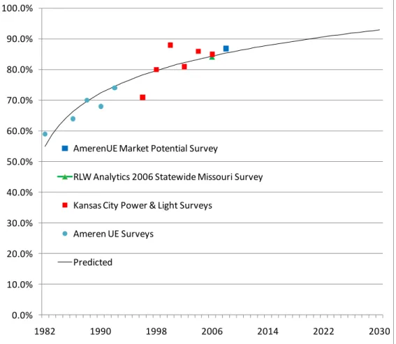
Figure 3.5: Air Conditioning Saturation, Survey Data Points and Fitted Curve
Three other sources of survey information were used to complement Ameren‟s Market Potential Study survey and make the process of developing the saturation trend time series easier and more accurate. One was a series of surveys conducted by Ameren Missouri (then Union Electric Company) of its service territory households between 1982 18 4 CSR 240-22.030(3)(B)1 0.0% 10.0% 20.0% 30.0% 40.0% 50.0% 60.0% 70.0% 80.0% 90.0% 100.0% 1982 1990 1998 2006 2014 2022 2030
AmerenUE Market Potential Survey
RLW Analytics 2006 Statewide Missouri Survey Kansas City Power & Light Surveys
Ameren UE Surveys Predicted
and 1992. Next, a series of surveys of its households conducted by Kansas City Power and Light between 1996 and 2006 and published publicly in their IRP document was used. The geographic proximity of KCP&L to Ameren Missouri is much better than the entire West North Central Census Region and the demographic make-up is more similar, and therefore it is a preferable source of secondary data to the EIA information. Finally, information from a statewide survey of Missouri households conducted by RLW Analytics in 2006 was also incorporated. The Ameren Market Potential Study was conducted in 2009, so a set of observations spanning the period between 1982 and 2009 was ultimately available. The approach used to develop the complete time series of saturation data for the historical and forecast period was to plot the points from all four survey sources and then fit a curve through the points. This methodology took advantage of all of the best information available and resulted in what is almost certainly a more accurate representation of the Ameren Missouri customer base than the regional EIA data. Figure 3.5 is a graph of this process for residential central air conditioning. In this case, one can see how this approach allows the incorporation of different survey data, and also allows us to incorporate a trend in saturation that is reasonable – in this case growth at a decreasing rate. In the example above for central air conditioning, this methodology predicted a saturation of 92.9% in 203019.
Appliance saturation and efficiency data is an obvious and important explanatory variable in modeling electricity sales, but there are other important variables that need to be included. Other logical predictors of electricity sales include the number of households in the service territory, income, and weather. Although this sales forecast is based on 30 year normal weather, actual historical weather is used to estimate model coefficients. In the SAE framework, elasticities with respect to price and income are determined exogenously and included in the calculation of the independent variables. The estimation of price and income elasticities is a complicated subject, and, especially with regard to price elasticity, there is a great deal of literature on the subject. One paper that was reviewed identified 36 different studies with 123 estimates of short run residential price elasticity, and those estimates ranged from -2.01 to -0.004. (Epsey, James A. and Molly Espey. “Turning on the Lights: A Meta-Analysis of Residential Electricity Demand Elasticities.” Journal of Agricultural and Applied Economics, 36, 1 (April 2004):65-81.). Ameren Missouri‟s approach to estimating elasticity parameters for each model was to
start with a figure that was close to a central tendency from the literature reviewed where possible, incorporating recommendations from the consultant firm Itron where necessary to supplement the available information20. After determining an appropriate starting point,
the elasticity parameters were then adjusted up or down by small amounts to determine
19 4 CSR 240-22.030(5)(B)2.C
whether model statistics improved from the change. The elasticities used in the base case load (the differences between the base, high, and low load growth scenarios are discussed in section 3.1.5) forecast models were values that minimized the model mean absolute percent error (MAPE) over the estimation period. The price elasticity in the base case load growth residential model is -0.15. This is also consistent with the value used in the 2008 Ameren Missouri IRP, which included a study of company specific data in a model that produced an estimate of -0.157 as reported in the Supplemental filing made by Ameren Missouri in that docket.
Ameren Missouri also considered the use of retail natural gas prices in the forecast as a competing fuel for certain end uses. After evaluating how the sales models performed with and without retail natural gas prices, retail natural gas prices were not included in the model as explanatory variables. When the natural gas prices were introduced to the forecasting model, a very strong trend appeared in the model residuals. Exclusion of the retail natural gas price produced slightly better model statistics and specifically an improved Durbin-Watson statistic which indicates a reduction in the correlation of the error term of the model (i.e. removal of gas prices eliminated the strong trend in the residuals).
Each model used a different economic driver, or a set of economic drivers. In the SAE model framework for residential sales, household income and the number of people per household in the service territory act as drivers for use per customer, and the number of households.
The functional framework of the SAE model is:
In each term the “index” variable captures past and future trends in appliance saturation and efficiency. The “use” variable is a combination of variables that characterize the utilization of the appliances, including household income, the number of people per household, heating & cooling degree days, and the relevant elasticities. The specific form of cooling use, for example, is:
The heating and other use variables are similar, except that the heating use variable includes heating degree days and the other use variable does not include a weather term. The coefficients B1, B2, and B3 are estimated with ordinary least squares (OLS) regression. One advantage of the SAE approach is that it produces very high, relative to most econometric models, t-statistics for each variable. In the base case residential model, for example, the t-statistics for the heating, cooling, and other variables are 55.68, 67.41, and 54.79 respectively. The adjusted r-square for that model is 0.987.
The SAE framework was also used for the four classes of commercial electricity sales: small general service (SGS), large general service (LGS), small primary service (SPS), and large primary service (LPS).
The functional form of the commercial SAE model is:
The coefficients B1, B2, and B3 were estimated with OLS regression.
The SAE approach used to forecast sales for the commercial rate classes is very similar to that used in the residential model. As with the residential class, the “index” variable includes past and forecasted data on appliance efficiency and saturation, while the “use” variable includes an economic driver, electricity prices, weather, and the appropriate elasticities. The commercial SAE model also includes building types and electric intensity that we matched to our customer base with data from the Ameren Missouri Market Potential Study.
One difference between the commercial class SAE models and the residential SAE model is that in the residential model the SAE function is used to forecast use per customer, and separate regression model predicts customers. Total MWh sales in the residential class are the product of the result of the customer model and the SAE model. In the case of the commercial class, we are forecasting MWh sales with the SAE models rather than use per customer.
Econometric
The four industrial rate classes were forecasted without including estimates of appliance saturation or efficiency that distinguish the SAE models from more traditional econometric models. The four industrial rate classes, small general service (SGS), large general service (LGS), small primary service (SPS), and large primary service (LPS) lack the homogeneity necessary to make the SAE approach useful. Across households, appliance use and saturation is fairly homogeneous, and even within the commercial class there is some homogeneity, especially within building types. Our industrial
customers are much less homogenous, however. The way that, for example, a brewery uses electricity is likely to be quite different from the way that an aircraft manufacturer uses electricity, and the way an aircraft manufacturer uses electricity is likely to be quite different from a cement factory.
In order to produce a forecast of energy that is reasonable and is able to incorporate future changes in the economic environment and electricity prices, it is necessary to include a price term, a price elasticity term, an economic driver, and some elasticity with respect to the economic driver in a sales model. The SAE framework does this very well, but as noted above that form is not appropriate for Ameren Missouri‟s industrial class sales. In a typical econometric model this would be done by including price and an economic driver in the model as independent variables. The regression estimated coefficients would then serve as de facto elasticities.
In the case of Ameren Missouri‟s industrial sales data, however, that approach does not always work, so a slightly different approach was used. Price in particular is problematic because real prices have trended flat to down over most of the estimation period of the sales models, and this tends to produce coefficients for the price term that are either statistically insignificant, practically insignificant (ie, a positive sign on the price coefficient), or both. A modification was chosen that combined price, output, and their respective elasticities into one composite independent variable.
The functional form was different from, but inspired by the SAE framework:
Price, output, and their elasticities were combined into one term. As was the case with the SAE residential and commercial models, estimating elasticity was a challenge, because estimates of elasticity in electricity consumption vary widely. Initial elasticities were chosen that reflected a mid-point of estimates from the literature. Through an iterative process elasticities were chosen that minimized the MAPE (Mean Absolute Percentage Error) over the sample period. A measure of billing or calendar days was added to the variable, to better reflect the volume of energy used in a month.
Obviously, the composite independent variable didn‟t include a weather term. In each rate class, an index of CDD and HDD were added as separate independent variables. In each of the four cases, the weather terms remained in the model if they were both practically and statistically significant.
Other
There are four other classes of energy sales which fell into neither the SAE nor econometric form of forecasting. Those four were Noranda, Street Lighting and Public Authority (SLPA), Dusk to Dawn lighting (DTD), and wholesale sales to cities and partial requirements customers. For Noranda sales (Noranda is an aluminum smelter which is its own rate class) the assumption is that they will operate at constant level, and require a constant amount of energy, for the foreseeable future. Noranda is part of a vertically integrated aluminum company, with its inputs coming from and outputs going to other parts of a common corporate parent. Load at Noranda would decline if the facility closed, and load could only expand if the facility were to add more production lines. The most likely case is that Noranda will continue to operate at its present capacity; if that assumption is correct then the only factor that will explain variation in monthly sales is the number of days in the month. Therefore Noranda sales are modeled as a function of the number of calendar days in the month.
Street lighting and public authority (SLPA) and dusk to dawn lighting (DTD) sales are both functions of the light in a day and other seasonal factors. We do not anticipate meaningful growth of sales in the DTD category; while we anticipate some very slight growth associated with population growth in the SLPA class. So the DTD classes are modeled such that monthly energy sales are functions of seasonal factors (specifically dummy variable for months) and the number of calendar days in the month. The SLPA class is similar, except that service territory population is included as an independent variable because we expect some slight growth dependent upon population growth.
Ameren Missouri served two types of wholesale customers at the time the IRP forecast was developed, full requirements municipal customers and partial requirements customers. The contracts for both types of customers expire during the IRP horizon. The partial requirements customers are AEP, an investor owned utility, and Wabash Valley Power Authority. For the partial requirements customers the forecasting process was straightforward; electricity sales were the product of the amount of capacity and energy called for by the contract.
For four municipal utilities, the cities of Perry, Kahoka, Marceline, and California, Ameren Missouri is the full provider of required electricity, as opposed to partially meeting their energy needs. For a fifth, the city of Kirkwood, Ameren Missouri is contracted as full provider for the term of one contract and then transitions to a partial provider under a second contract for an additional term. Sales to these five customers were modeled econometrically, but the process was not the same as that used for Ameren Missouri‟s
retail sales. This was partially because the cities include a mix of customer types, rather than being strictly residential or commercial, although a majority of the load is residential. The independent variables in those sales models were GDP and persons per household.
Since an exact tabulation of GDP and persons per household was not available for those five, relatively small cities, the corresponding value for Ameren Missouri‟s service territory was used. This is defensible as the five cities are within Ameren Missouri‟s service territory, and we have no reason to expect a systematic and sustained difference between the economic performance of those five cities and the Ameren Missouri service territory. Customer History and Forecasts
Forecasts of customer counts were produced at the rate class level, although in charts and tables they are aggregated to revenue class21. In each case, an econometric
approach was used with customers modeled as a function of an appropriate driver, such as households, employment, or GDP22. Normally this would be a straight forward process, but it was complicated by the fact that GDP and employment both contracted rather severely in 2008 and 2009, and to a greater extent than the number of customers did. There was a similar, but opposite problem in the residential class, as the growth in households under-predicted the rate of residential customer growth between 2003 and 2008 (the period now recognized as a housing bubble). The customer models therefore included dummy variables to capture the fact that customer growth and driver growth diverged over the last few years, and also included auto-regressive and moving average terms to smooth out the customer forecast.
3.1.5 Sensitivities and Scenarios
23The nature of the forecasting models used in this IRP forecast is such that the dependent variable (energy sales) is sensitive to changes in the independent variables as well as to the parameter estimates used to represent elasticity. This is a feature of econometric and SAE models, but it is worth mentioning here because it means that the forecast of energy sales is highly sensitive to changes in any one of the driver variables. The forecast of residential sales is sensitive to changes in households, electricity prices, income, population, and changes in appliance saturation and efficiency. Commercial and industrial sales are sensitive to changes in service territory GDP, employment, electricity prices.
In this IRP, ten different scenarios were modeled that stemmed from the permutations of independent assumptions about load growth (low, medium, high24), natural gas prices
(high, base, or low), and carbon prices (no carbon policy, energy bill mandates, EPA regulation, or a cap and trade system). Charles River Associates (CRA) produced different forecasts of retail electricity prices to match each permutation. They also produced forecasts of national and regional economic conditions associated with those scenarios that were used to adjust the Ameren Missouri service territory specific
21 4 CSR 240-22.030(5)(B)1 22 4 CSR 240-22.030(2)
23 4 CSR 240-22.030(6), 4 CSR 240-22.030(7), 4 CSR 240-22.030(8)(C) 24 EO-2007-0409 – Stipulation and Agreement #13
assumptions used in the modeling. CRA developed these forecasts based on interviews with Ameren subject matter experts, and results of the interviews were translated in to quantitative forecasts. The overall scenario development process is discussed fully in Chapter 2.
The different carbon policy and natural gas price scenarios affected the forecasts of energy sales through the retail price term and economic drivers, as changes in wholesale natural gas prices and regulatory regimes flowed through CRA‟s model to set different
levels and growth rates of retail electricity prices and different national and regional economic conditions. Since the retail price of electricity and economic drivers are inputs into the sales models (both SAE and econometric), the different carbon and natural gas scenarios result in different forecasts of energy sales25. Additionally, the energy bill mandates cases included some assumptions regarding new future federal energy efficiency standards that were implemented in the SAE framework.
In order to forecast high, base and low load growth consistent with the scenarios envisioned by the load growth subject matter experts, Ameren Missouri developed different levels of selected independent variables and elasticity parameters. The variables and parameters that were selected to be varied in the scenario forecasts differed by class. In each case, it was important to consider not only which variable or parameter had the biggest impact on load, but also which ones had the greatest inherent uncertainty over the planning horizon.
For example, in the residential model the forecast of miscellaneous end use energy was modified to produce high and low load growth scenarios. Miscellaneous load is generally considered to be one of the most challenging categories to forecast amongst industry forecasters. Since miscellaneous load makes up a significant share of total residential energy consumption (approximately 20% in 2010), changes in the growth rate of this end use grouping will certainly have a material impact on the load forecast. Implied in the EIA information is a historical trend in miscellaneous growth that in individual years is over 5% and for a sustained period of time exceeded 3%. However, over the forecast period, EIA‟s forecast implies reductions in miscellaneous load growth such that it remains in only the 1-1.5% range. The difference between the historical and forecast EIA trends alone make meaningful differences in the total residential load forecast. Part of the appeal of miscellaneous growth as the variable through which to capture uncertainty is its inherent unpredictability. It is impossible to know what new devices might be invented in the future that will consume more or less electricity than what is currently anticipated. A forecast of 2010 energy sales prepared in 1990 for example, might have underestimated the number of mobile phone chargers, not have predicted the adoption of technologies like digital video recording devices, or not have expected that some households would have a
device called a wireless router. It is also conceivable that technologies could converge in the future and multiple plug devices are replaced by more efficient and fewer devices. Electric vehicles (EVs) are another example of a category of miscellaneous sales growth that could affect the forecast of energy sales. It is also a category of sales about which there is a great deal of uncertainty. Ameren Missouri has and continues to research the potential of plug in EVs as a source of load growth, but at present the state of technology leads to a wide spectrum of possible outcomes. Currently Ameren Missouri does not see the likelihood of electric vehicle sales reaching levels high enough to meaningfully affect electricity sales in the near to medium term, as a survey of Ameren Missouri customers showed that 65% of respondents described themselves as “not very likely” to buy an electric or hybrid electric car. Only 8% of respondents characterized themselves as “very likely” to purchase such a vehicle.
Under an aggressive scenario envisioned where electric vehicle production ramped up significantly such that the market penetration of EVs reached 15% as fast as 2015 and 25% by 2020, the total estimated impact to residential load would only be about 4%. That means that if EVs take off immediately, load growth from 2010 to 2020 would only be 0.4% per year higher. However, over the entire IRP planning horizon, it is easily conceivable that EVs could provide much of the growth envisioned in the high load growth case.
For the commercial class, the output and price elasticity parameter estimates were identified as the largest source of uncertainty for the forecast period. As mentioned in Section 3.1.4, the academic literature and even the opinions of the forecasting community present a wide spread of supportable estimates of elasticity. However, much of the literature that does cover elasticity actually focuses on the residential class. Therefore the evidence for a single parameter estimate for Commercial price or output elasticity is scarce. The impact of these estimates is, however, significant. Since we are in a time period during which retail electric prices have been and are forecasted to continue rising, the price elasticity term has a pronounced effect.
Additionally, economic growth in the commercial sector is not uniformly energy intensive. So the addition of load like data centers and medical facilities could use more energy per unit of economic output than retail space or offices. Therefore using the output elasticity to model sensitivity accurately captures one of the larger uncertainties in this sector. The industrial class had three different variables/parameters that were affected in the load growth scenario modeling. First, similar to the commercial class, different output and price elasticity parameters were introduced across the cases for reasons similar to those described for the commercial class. Second, the handling of the recovery from the severe recession in 2007-2009 was handled differently across scenarios. In the high and base
growth cases, a modeling technique was used that produced more of a “V” recovery. This is how many past recessions have occurred, with economic decline being followed by a period of above trend growth that quickly brings the economy close to where it was pre-recession. In the low load growth scenario, the recession variable in the model did not indicate a rapid recovery, and a permanent loss in load was the ultimate effect.
The final mechanism used to differentiate the load growth cases in the industrial class models was the choice of economic driver variables. As discussed earlier, both manufacturing output and manufacturing employment correlate with electricity sales. The key difference between the two in this forecast, however, is that Moody‟s Analytics‟
forecast of Ameren Missouri‟s service territory activity predicts growth in manufacturing output but declining manufacturing employment. This is not an illogical outcome; it merely implies manufacturing productivity growth at a rate greater than the growth of output. That logic non-withstanding, the choice of employment as opposed to output as a driver has big implications for electricity sales in the future. If industrial sales are driven by output then Ameren Missouri‟s industrial energy sales will grow over the IRP horizon, but if they are instead driven by manufacturing employment they will decline.
For our base case, we essentially split the difference by creating an industrial output index that was the average of indexed levels of manufacturing employment and output. The rationale for this combination is that in some instances electricity consumption will be a complement to employment, but in others it will be a substitute for employment. Some industries will cut their employment and electricity use as their output grows, while others will cut employment but increase use. For the high load growth case the assumption is that manufacturers in the region become more efficient by replacing labor with electricity intensive capital, while for the low load case the assumption is that manufacturers become more efficient users of both labor and electricity, so their use of both declines as output grows.
As described in the paragraphs above, careful consideration was given to the factors in the forecast of each class that would drive the differences between the high, base, and low load forecast scenarios. In each case, an assessment was made that not only considered the model‟s sensitivity to a given variable, but also the inherent uncertainty in that variable. By using this approach, Ameren Missouri developed a range of load growth outcomes that realistically reflects the uncertainty that is truly present in the details underlying the load forecasting process. The results of this modeling served to reinforce the results of the surveys that CRA conducted with the subject matter experts.
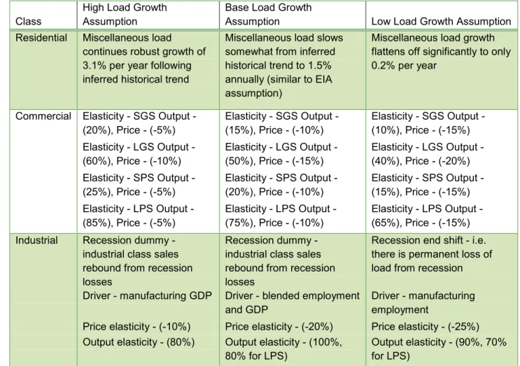
A summary detailing all of the changes between high, base, and low load forecast scenarios can be found in Table 3.3.
Table 3. 3: Scenario Driver and Parameter Differences
Class High Load Growth Assumption Base Load Growth Assumption Low Load Growth Assumption Residential Miscellaneous load
continues robust growth of 3.1% per year following inferred historical trend
Miscellaneous load slows somewhat from inferred historical trend to 1.5% annually (similar to EIA assumption)
Miscellaneous load growth flattens off significantly to only 0.2% per year
Commercial Elasticity - SGS Output -
(20%), Price - (-5%) Elasticity - SGS Output - (15%), Price - (-10%) Elasticity - SGS Output - (10%), Price - (-15%) Elasticity - LGS Output -
(60%), Price - (-10%) Elasticity - LGS Output - (50%), Price - (-15%) Elasticity - LGS Output - (40%), Price - (-20%)
Elasticity - SPS Output -
(25%), Price - (-5%) Elasticity - SPS Output - (20%), Price - (-10%) Elasticity - SPS Output - (15%), Price - (-15%) Elasticity - LPS Output -
(85%), Price - (-5%) Elasticity - LPS Output - (75%), Price - (-10%) Elasticity - LPS Output - (65%), Price - (-15%) Industrial Recession dummy -
industrial class sales rebound from recession losses
Recession dummy - industrial class sales rebound from recession losses
Recession end shift - i.e. there is permanent loss of load from recession Driver - manufacturing GDP Driver - blended employment
and GDP Driver - manufacturing employment Price elasticity - (-10%) Price elasticity - (-20%) Price elasticity - (-25%) Output elasticity - (80%) Output elasticity - (100%,
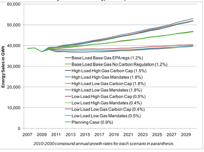
Figure 3.6: Total Energy Sales by Scenario
3.1.6 Planning Case Forecast
26The ten scenarios described in section 3.1.5 describe the range of likely outcomes for load growth over the planning horizon. The single forecast that represents the expected value of load growth over the planning horizon is referred to as the planning case. This forecast is needed in order to have a base expectation against which the candidate resource plans can be developed. The integration modeling is actually run against each scenario forecast, but the plans were created in order to maintain an appropriate amount of capacity given expectations in the planning case.
The initial calculation of the planning case forecast was a fairly simple exercise. The subjective probabilities of each scenario, as determined by the subject matter experts for the various uncertain factors, were used to weight together the different scenarios. The planning case did not have its own set of forecast models with case specific drivers, but instead was derived from the modeling results for all other scenarios.
26 4 CSR 240-22.030(5), 4 CSR 240-22.030(5)(A) 0 10,000 20,000 30,000 40,000 50,000 60,000 2007 2009 2011 2013 2015 2017 2019 2021 2023 2025 2027 2029 E n e rg y S a le s in G W h
Base Load Base Gas EPA regs (1.2%)
Base Load Base Gas No Carbon Regulation (1.2%) High Load High Gas Carbon Cap (1.5%)
High Load High Gas Mandates (1.8%) High Load Low Gas Carbon Cap (1.8%) High Load Low Gas Mandates (1.8%) Low Load High Gas Carbon Cap (0.5%) Low Load High Gas Mandates (0.4%) Low Load Low Gas Carbon Cap (0.4%) Low Load Low Gas Mandates (0.5%) Planning Case (0.9%)
Following completion of the original planning case calculation as described above, but before integration analysis had begun in earnest, a review was undertaken to determine how well the forecast was performing against first quarter 2010 observed weather normalized loads. Because there is a very long lead time required to prepare all of the load analysis and forecasting work, the forecast assumptions are a few months old before the forecast is even used. There was a short window of opportunity to get updated information into the forecast, and Ameren Missouri chose to take one last look at it before proceeding with integration analysis.
It turns out that the forecast for the first quarter was significantly lower than the observed loads were coming in. Specifically, total weather normalized load was 2.7% higher than the forecast. This was most pronounced in the residential class which was 5.7% above the original planning case forecast.
Ameren Missouri determined that, although it was very confident in the subjective probabilities over the duration of the planning horizon, due primarily to the observed deviation of the actual load to the forecast, the high case load growth was more likely in the very near term. To reflect this reality, an additional model was executed that included the base load and base gas assumptions, but that incorporated for the most part the high load growth assumptions27. This additional model also incorporated 2010 loads through May in
the estimation and weather normalized observed first quarter 2010 loads through April in the results.
The results of the new model described above were utilized for the planning case for the first two years (recall the near term expectation for high load growth described above). After 2011, the annual growth rates from the original planning case were applied to the level of sales in 2011 produced by these new models on a class by class basis.
3.1.7 Forecast Results
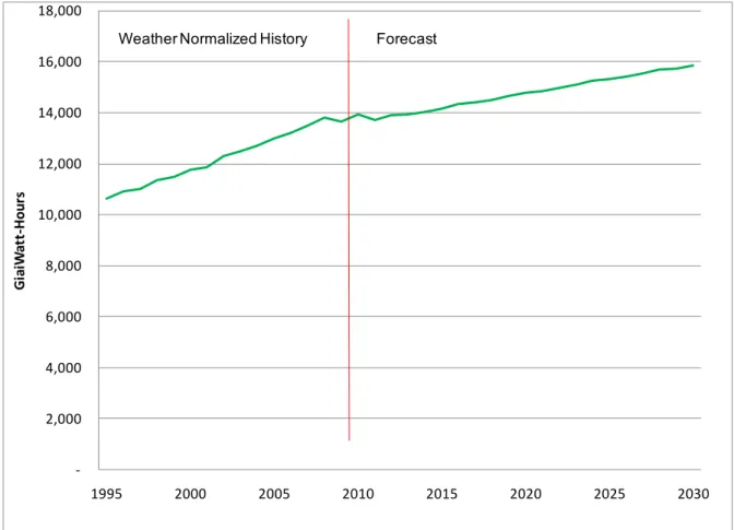
28For the planning case, total retail energy sales are forecast to grow at 1.09% compound annual rate between 2010 and 2030. Between 1996 and 2009, total retail sales grew at a compound annual rate of 2.2%. Sales dipped sharply in 2009, but are expected to recover in 2010 and 2011 and then grow at a relatively stable and slow rate through 2030. Because of expiring wholesale contracts that cause and artificial decline in load, Ameren Missouri‟s total load obligation is expected to grow by only 0.94% per year from 2010 to 2030.
27 The industrial class forecast for the revised planning case did not fully incorporate the high load growth
assumptions. Specifically, it was modeled with a “fuzzy” recession variable. This in effect produced neither a “V” recovery in industrial load nor a permanent load loss, but a slower recovery of load to pre-recession levels.
Sales increased noticeably in 2005 when Ameren Missouri began serving the Noranda aluminum smelting facility. In 2009 an ice storm caused the failure of some transmission lines (not owned by Ameren Missouri) that served the plant, and the resulting power outage damaged the plant. It did not return until full capacity until mid 2010.
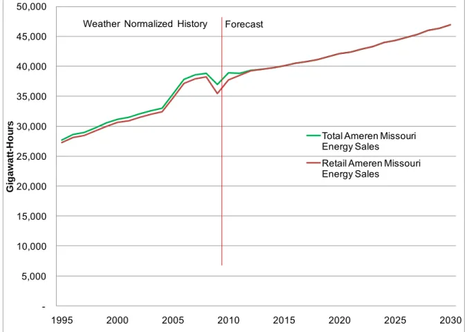
Figure 3.7: Planning case energy sales forecast
The outage at Noranda is not the only reason why sales slumped in 2009, however, as the severe recession that the US experienced depressed service territory electricity sales. Residential sales fell by 1.3% in 2009, commercial sales fell by 1.5%, and Industrial sales, exclusive of Noranda, fell by a staggering 14.5%. The planning case assumes that recovery from those declines takes several years, as can be seen in Figure 3.7.
-5,000 10,000 15,000 20,000 25,000 30,000 35,000 40,000 45,000 50,000 1995 2000 2005 2010 2015 2020 2025 2030 G ig a w a tt -H o u rs
Total Ameren Missouri Energy Sales
Retail Ameren Missouri Energy Sales
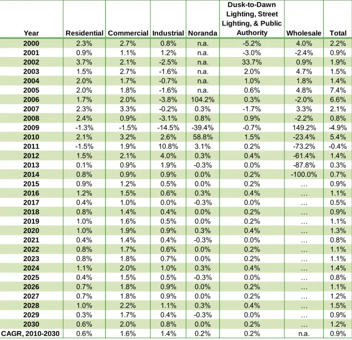
Table 3.4: Planning Case Annual Sales Growth by Class
One seemingly trivial feature of our sales modeling does impact sales growth. In each of our models, the number of calendar days in the month is included as an explanatory variable; either on its own or combined with another. Each leap year is one day, or 0.27% longer than normal, and that extra day is in a month when we typically experience meaningful heating load. That causes sales growth in every leap year to be slightly higher than it otherwise would be, and growth in each year that follows a leap year to be slightly lower. This isn‟t noticeable in Figure 3.6, but is noticeable in Table 3.4. The effect of leap
years on sales is in one sense trivial, and doesn‟t meaningfully affect capacity planning, which is of course the central goal of the IRP. It is, however, a logical and observable result of the forecasting process.
Year Residential Commercial Industrial Noranda
Dusk-to-Dawn Lighting, Street Lighting, & Public
Authority Wholesale Total
2000 2.3% 2.7% 0.8% n.a. -5.2% 4.0% 2.2% 2001 0.9% 1.1% 1.2% n.a. -3.0% -2.4% 0.9% 2002 3.7% 2.1% -2.5% n.a. 33.7% 0.9% 1.9% 2003 1.5% 2.7% -1.6% n.a. 2.0% 4.7% 1.5% 2004 2.0% 1.7% -0.7% n.a. 1.0% 1.8% 1.4% 2005 2.0% 1.8% -1.6% n.a. 0.6% 4.8% 7.4% 2006 1.7% 2.0% -3.8% 104.2% 0.3% -2.0% 6.6% 2007 2.3% 3.3% -0.2% 0.3% -1.7% 3.3% 2.1% 2008 2.4% 0.9% -3.1% 0.8% 0.9% -2.2% 0.8% 2009 -1.3% -1.5% -14.5% -39.4% -0.7% 149.2% -4.9% 2010 2.1% 3.2% 2.6% 58.8% 1.5% -23.4% 5.4% 2011 -1.5% 1.9% 10.8% 3.1% 0.2% -73.2% -0.4% 2012 1.5% 2.1% 4.0% 0.3% 0.4% -61.4% 1.4% 2013 0.1% 0.9% 1.9% -0.3% 0.0% -87.8% 0.3% 2014 0.8% 0.9% 0.9% 0.0% 0.2% -100.0% 0.7% 2015 0.9% 1.2% 0.5% 0.0% 0.2% … 0.9% 2016 1.2% 1.5% 0.6% 0.3% 0.4% … 1.1% 2017 0.4% 1.0% 0.0% -0.3% 0.0% … 0.5% 2018 0.8% 1.4% 0.4% 0.0% 0.2% … 0.9% 2019 1.0% 1.6% 0.5% 0.0% 0.2% … 1.1% 2020 1.0% 1.9% 0.9% 0.3% 0.4% … 1.3% 2021 0.4% 1.4% 0.4% -0.3% 0.0% … 0.8% 2022 0.8% 1.7% 0.6% 0.0% 0.2% … 1.1% 2023 0.8% 1.8% 0.7% 0.0% 0.2% … 1.1% 2024 1.1% 2.0% 1.0% 0.3% 0.4% … 1.4% 2025 0.4% 1.5% 0.5% -0.3% 0.0% … 0.8% 2026 0.7% 1.8% 0.9% 0.0% 0.2% … 1.1% 2027 0.7% 1.8% 0.9% 0.0% 0.2% … 1.2% 2028 1.0% 2.2% 1.1% 0.3% 0.4% … 1.5% 2029 0.3% 1.7% 0.4% -0.3% 0.0% … 0.9% 2030 0.6% 2.0% 0.8% 0.0% 0.2% … 1.2% CAGR, 2010-2030 0.6% 1.6% 1.4% 0.2% 0.2% n.a. 0.9%
Residential29
Between 1996 and 2009, residential class weather normalized sales grew at a compound annual rate of 1.8%. Total US residential sales, according to the EIA, also grew by 1.8% (although it is important to note that EIA numbers are not weather normalized), so Ameren Missouri‟s residential electricity consumption growth was similar to the US as a whole.
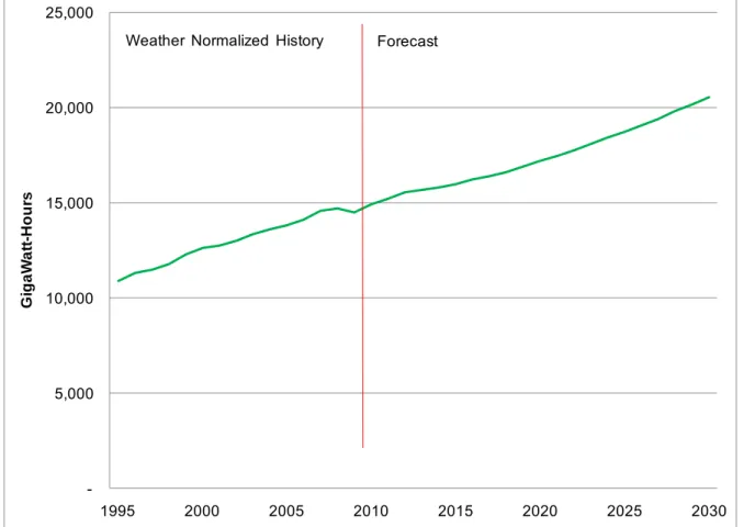
Figure 3.8: Planning Case Forecast of Residential Energy Sales
In the planning case forecast, that growth slows to a compound annual rate of 0.6% between 2010 and 2030 because of higher electric rates, slower growth in households, and increasing adoption of energy efficient technologies. According to the EIA, US residential electricity sales are expected to grow at a compound annual rate of 0.8% over the same time period. The slightly lower growth of Ameren Missouri electricity sales is consistent with the idea that the Ameren Missouri service territory will experience slightly slower demographic growth than the US in the long term.
In the near term, sales will decline in 2011. This is due to the inclusion of the weather normalized observed results for the first quarter of 2010 in the updated planning case. As 29 4 CSR 240-22.030(5)(A) -2,000 4,000 6,000 8,000 10,000 12,000 14,000 16,000 18,000 1995 2000 2005 2010 2015 2020 2025 2030 G ia iW at t-Ho u rs
mentioned above, particularly high load growth was observed in this period (which led to the decision to update the planning case). Although these months were also included in the estimation of the planning case forecast model, the three additional months of strong load were not enough to force the model to repeat this level of load in 2011. Therefore returning to a more “normal” winter sales level in 2011 actually caused a reduction in load compared with 2010. Additionally, a significant rate increase in June 2010 drives conservation impacts in 2011 through the 1 year moving average of price treatment in the model described just below. The surge in growth in 2012 is due to an expected rebound in household formation. In 2013 the effects of efficiency standards partially offset favorable economic trends. Growth is robust, again due to higher rates of household formation and income growth, through 2016, but then decelerates over time. The effect of higher prices also depresses sales growth. Prices were relatively flat in real terms between 1995 and 2008, but began to rise in 2009. The forecasting models use a 1-year moving average of prices because we believe that although prices rise immediately after a rate case, our customers respond more slowly. That means that the demand reducing effects of higher prices show up over the year following the rate increase.
The number of residential customers is expected to grow at a compound average rate of 0.8% between 2010 and 2030. Customers grow more rapidly, at a rate of 1.5%, between 2010 and 2015 as a recovery from the 2007-2009 recessions spurs an above trend rate of household formation. Between 2015 and 2030 growth slows to 0.5% as slow demographic growth leads to low rates of household formation.
Use per customer growth in the residential class is expected to slow relative to historical trends. Over the 1995-2009 time period, user per customer grew at approximately 1.1%. Over the forecast horizon, use per customer is expected to be very close to flat, with all usage growth coming from a modestly increasing customer base30.
Commercial31
Ameren Missouri commercial class sales are the fastest growing segment of sales, partially reflecting the shift away from manufacturing toward health and education in the service territory economy, and partially because of the growth of new types of commercial load such as data centers. Between 1996 and 2009, weather normalized sales grew at a compound annual rate of 2.0%. According to the EIA, total US commercial sales grew at a compound annual rate of 3.1% between 1996 and 2001, so Ameren Missouri‟s growth was slower than the US average.
Sales are expected to grow at a compound annual rate of 1.6% between 2010 and 2030. The EIA‟s estimate of commercial electricity sales growth over that same period is 1.8%,
30 4 CSR 240-22.030(5)(B)2.D 31 4 CSR 240-22.030(5)(A)
so the planning case for Ameren Missouri anticipates slightly slower growth that the US average.
Use per customer growth in the commercial class has been negligible over the historical period of 1995-2009 with growth being driven by an increasing customer base. This trend is expected to continue, with essentially flat commercial use per customer over the forecast horizon32.
Figure 3.9: Planning Case Forecast of Commercial Class Energy Sales
Industrial33
Ameren Missouri Industrial class sales grew at a compound annual average rate of 2.0% between 1995 and 2001, before a structural decline in service territory manufacturing output began to depress sales. The decline in manufacturing activity was not one confined to the Ameren Missouri service territory; between 2001 and 2009, manufacturing employment fall by 27.7% nationwide, 31.7% in the State of Missouri, and by 25.9% in the St. Louis metropolitan area.
32 4 CSR 240-22.030(5)(B)2.D 33 4 CSR 240-22.030(5)(A) -5,000 10,000 15,000 20,000 25,000 1995 2000 2005 2010 2015 2020 2025 2030 G ig a W a tt -H o u rs
Casualties of this secular decline in the service territory include the Ford Assembly plant in Hazelwood, MO, which closed in 2003, and the Chrysler plant in Fenton MO, which closed in 2010. Between 2001 and 2009, Ameren Missouri‟s Industrial sales declined at a compound annual rate of 3.6%; according to the Energy Information Administration US industrial electricity sales fell by a compound annual rate of 1.5% between 2001 and 2009. The fact that Ameren Missouri‟s sales declines are larger than the US is partly due
to the complete loss of the large customers mentioned above.
Figure 3.10: Planning Case Forecast of Industrial Class Energy Sales
The planning case forecast calls for industrial sales growth at a compound annual rate of 1.4% between 2010 and 2030. That may seem aggressive given the decline in sales since 2001, but it is also the case that the forecast does not anticipate that industrial sales will reach 2001 levels until after 2030. The EIA‟s forecast for US industrial sales anticipates compound annual growth of 0.8%, slower than the planning case forecast. The difference between the planning case forecast for Ameren Missouri and the EIA‟s is primarily due to Moody‟s Analytics‟ fairly robust forecast of manufacturing activity in the service territory, which calls for manufacturing GDP to grow at a compound annual rate of 3.4% between 2010 and 2030. The EIA, on the other hand, sees shipments of manufactured goods (an analogous but not identical measure to manufacturing GDP) to grow at a compound annual rate of 2.3%.
-1,000 2,000 3,000 4,000 5,000 6,000 7,000 1995 2000 2005 2010 2015 2020 2025 2030 G ia iW a tt -H o u rs
The earlier discussion of forecast drivers detailed the difference that the use of manufacturing output as opposed to employment as a forecast driver has on manufacturing sales. The base load growth case forecast essentially splits that difference, using an equally weighted blend of the growth of manufacturing employment and GDP.
While total sales declined over the historical period from 1995-2009, this was driven primarily by a declining customer base. Use per customer actually grew at 0.6% per year over the same years. Over the forecast horizon, that is expected to continue and actually accelerate. Use per customer is forecast to grow by 1.8% per year as output expands despite declining employment in the sector34.
CustomerForecast
The forecasts of customers for the residential, commercial and industrial classes are reasonable given the performance of customer growth over the prior decade and a half35.
For the residential class, forecasted growth rates are very close to the rate of the past fifteen years. For the commercial class, we expect growth to decelerate slightly. The commercial class does remain the fastest growing retail class, however.
Table 3.5: Customer Growth Rates
Year Residential Commercial Industrial
1995-2009 0.73% 2.21% -1.83% 2010-2030 0.77% 1.50% -0.38%
The number of industrial customers decline at a slower rate over the forecast horizon than it is over the last fifteen years by a significant margin, over 140 basis points. This is primarily because the Ameren Missouri service territory has experienced a secular decline in manufacturing over the last several decades, but we believe that decline is slowing. This is partially because the sustained declines in industrial customers are leaving a customer base that is more concentrated with competitive firms that are more likely to survive.
Wholesale36
Ameren Missouri sells electricity to five full requirements wholesale customers; the cities of California, Kahoka, Kirkwood, Marceline, and Perry, and two partial requirements wholesale customers; AEP and Wabash Valley. At the time of the forecast, Ameren Missouri anticipated, because of existing contracts, sales to Kahoka and Marceline to continue through December of 2011, sales to Kirkwood to extend through August of 2012, sales to California through May of 2013, and sales to Perry to continue through 2013.
34 4 CSR 240-22.030(5)(B)2.D
35 4 CSR 240-22.030(5)(B)1.B, EO-2007-0409 – Stipulation and Agreement #12 36 4 CSR 240-22.030(5)(A)