ScholarWorks@UNO
ScholarWorks@UNO
Computer Science Faculty Publications Department of Computer Science
10-2015
DisPredict: A Predictor of Disordered Protein Using Optimized RBF
DisPredict: A Predictor of Disordered Protein Using Optimized RBF
Kernel
Kernel
Sumaiya Iqbal
University of New Orleans
Md Tamjidul Hoque
University of New Orleans
Follow this and additional works at: https://scholarworks.uno.edu/cs_facpubs
Part of the Bioinformatics Commons Recommended Citation
Recommended Citation
Iqbal S, Hoque MT (2015) DisPredict: A Predictor of Disordered Protein Using Optimized RBF Kernel. PLoS ONE 10(10): e0141551. doi:10.1371/journal.pone.0141551
This Article is brought to you for free and open access by the Department of Computer Science at
ScholarWorks@UNO. It has been accepted for inclusion in Computer Science Faculty Publications by an authorized administrator of ScholarWorks@UNO. For more information, please contact [email protected].
DisPredict: A Predictor of Disordered Protein
Using Optimized RBF Kernel
Sumaiya Iqbal, Md Tamjidul Hoque*
Department of Computer Science, University of New Orleans, New Orleans, LA, United States of America
Abstract
Intrinsically disordered proteins or, regions perform important biological functions through their dynamic conformations during binding. Thus accurate identification of these disor-dered regions have significant implications in proper annotation of function, induced fold prediction and drug design to combat critical diseases. We introduce DisPredict, a disorder predictor that employs a single support vector machine with RBF kernel and novel features for reliable characterization of protein structure. DisPredict yields effective performance. In addition to 10-fold cross validation, training and testing of DisPredict was conducted with independent test datasets. The results were consistent with both the training and test error minimal. The use of multiple data sources, makes the predictor generic. The datasets used in developing the model include disordered regions of various length which are categorized as short and long having different compositions, different types of disorder, ranging from fully to partially disordered regions as well as completely ordered regions. Through com-parison with other state of the art approaches and case studies, DisPredict is found to be a useful tool with competitive performance. DisPredict is available athttps://github.com/ tamjidul/DisPredict_v1.0.
1 Introduction
Many protein regions and some entire proteins do not adopt well-defined, stable three-dimensional (3D) structures in an isolated state and under different non native environments
[1–3]. These proteins or partial regions of proteins are called intrinsically disordered proteins
(IDPs) or disordered regions in proteins (IDRs), also known as natively unstructured, dena-tured or unfolded. The coordinates of their backbone atoms have no specific equilibrium states and can vary largely due to variable physiological conditions, and thus adopt dynamic structural ensembles. Structurally, IDPs (or IDRs) encompass proteins or protein-regions with extended disorder, collapsed disorder and semi-collapsed disorder. These reflect differ-ences in the underlying biophysical characteristics including low hydrophobicity and high
net charge, marginal level of residual secondary structure [4,5], dynamic side chains and
sec-ondary structures [6,7], rapidly exchanging backbone side-chain hydrogen bonds which
make a region unable to form specific secondary structure [3]. Recognition of these protein
OPEN ACCESS
Citation:Iqbal S, Hoque MT (2015) DisPredict: A Predictor of Disordered Protein Using Optimized RBF Kernel. PLoS ONE 10(10): e0141551. doi:10.1371/ journal.pone.0141551
Editor:Alexandre G. de Brevern, UMR-S665, INSERM, Université Paris Diderot, INTS, FRANCE Received:January 4, 2015
Accepted:October 9, 2015 Published:October 30, 2015
Copyright:This is an open access article, free of all copyright, and may be freely reproduced, distributed, transmitted, modified, built upon, or otherwise used by anyone for any lawful purpose. The work is made available under theCreative Commons CC0public domain dedication.
Data Availability Statement:All relevant data are available via GitHub (https://github.com/tamjidul/ DisPredict_v1.0.git) as well as via the University of New Orleans, Department of Computer Science website (http://cs.uno.edu/*tamjid/Software/ DisPredict/DisPredict_v1.0.tar.gz).
Funding:SI and MTH gratefully acknowledge the Louisiana Board of Regents through the Board of Regents Support Fund, LEQSF (2013–16)-RD-A-19. Competing Interests:The authors have declared that no competing interests exist.
disordered regions is important for appropriate protein structure prediction, disease causing protein identification, proper annotation of function, induced folding and binding region prediction.
For the last two decades, many works have been presented in evidence that many proteins do not follow the well-known paradigm of sequence to stable structure to function. Rather
these proteins adopt disordered state for complex and essential biological functions [1,6,8,
9] such as cell cycle control and cellular signal transduction, transcriptional and translational
regulation, membrane fusion and control pathways [1,10,11]. They participate in molecular
recognition, molecular assembly and protein modification [12,13] via protein-protein,
pro-tein-nucleic acid and protein-ligand interactions as well. Disorder proteins are found to be
highly associated with critical human diseases [14–16], such as cancer, amyloidoses,
cardio-vascular and neurodegenerative diseases, genetic diseases. Thus, identifying them assists in
effective drug development [17,18].
In reality the IDPs are abundant. Approximately 70% of the structures released by Protein
Data Bank (PDB) [19] contain some disordered residues [20,21]. A curated database of
disor-dered proteins, called DisProt [22] contains annotation for 694 protein sequences and 1539
disordered regions in its current version 6.02. The IDEAL [23,24] and MobiDB [25,26]
data-bases also provide useful collections for annotation of intrinsic disorder. PDB [19] database,
which gives provision of finding disordered regions in the solved secondary or tertiary struc-ture incorporates 105,097 protein entries. To compare, the overall number of non-redundant protein sequences is 46,968,574 according to the most recent 68 release of RefSeq database
[27]. However, due to highly flexible characteristics of the residues of IDRs or, IDPs [28]),
experimentally verified annotation of intrinsic disorder is growing slowly. Thus to keep pace with this large-scale increase in protein database, effective computational methods for correct identification of disordered residues in IDPs or, IDRs are necessary.
Several computational methods have been developed to fulfill the fast annotation require-ments for the rapidly growing known protein sequences. Machine learning based some of these
well-known approaches are PONDR series [20,29,30], DISOPRED [31], DISOPRED2 [32],
DisEMBL [33], DISpro [34], RONN [35], Spritz [36], PROFbval [28,37], DisPSSMP [38,39],
PrDOS [40], POODLE series [41,42], NORSnet [43], IUP [44], OnD-CRFs [45], PreDisOrder
[46], SPINE-D [47] and ESpritz [48]. Several existing tools, for instance GlobPlot [49], IUPred
[50], FoldIndex [51] and Ucon [52], usage knowledge such as the relative composition and
pro-pensity of amino acids. On the other hand, DISOclust [53] is based on the analysis of how
dis-order is related with protein folding and uses predicted three-dimensional structural
characteristics. Combination of individual methods in a complementary method gave raise to
effective disorder predictors, such as metaPrDOS [54], MD [55], MFDp [56], PONRD-FIT
[21] and very recent MFDp2 [57].
In this article, we propose a new disorder predictor, named“DisPredict (Disorder
Predictor)”[58]. DisPredict classifies ordered and disordered residues in a protein sequence
with higher accuracy, specifically in terms of Mathews Correlation Coefficient (MCC) and Area Under the receiver operating characteristics Curve (AUC). Dispredict is based on Sup-port Vector Machine (SVM) using Radial Basis Function (RBF) as kernel. We further strengthened the classification performance of DisPredict by selecting optimized parameters of SVM which significantly improved the performance. We utilized a comprehensive set of
56 features to characterize disorder in protein sequence. We compared DisPredict’s
perfor-mance with existing predictors, SPINE-D [47] and MFDp [56], followed by an analysis of its
performance with respect to different types of amino acid, length of disorder region and datasets.
2 Materials and Methods
In this section, we discuss the data-sources, data-processing, input-feature generations, soft-ware design and platform and performance evaluation.
2.1 Preliminary Disordered Data Sources
In the prior studies, PDB [19] and DisProt [22] are considered as the primary repositories of
IDPs. Disorder regions are composed of residues with missing coordinates in structure solved by X-ray crystallography, whereas the residues show highly variable coordinates within ensem-ble solved by NMR. We selected two datasets which combine sequences from PDB having dis-ordered residues without coordinates (recorded in REMARK 465) and sequences from DisProt, having curated annotations of disorder regions including properties such as short
(30 residues) and long (>30 residues) disordered regions, partial as well as fully ordered or
disordered chains.
2.2 Datasets
We used two different datasets, MxD and SL, to train, test and cross-validate our proposed
Dis-Predict. MxD and SL datasets were used to train two disorder predictors, SPINE-D [47] and
MFDp [56], respectively. We collected and utilized these datasets to be able to consistently
compare DisPredict with these two predictors.
The Mixed Disorder (MxD) dataset is a combination of protein sequences with disordered
residues from both PDB and DisProt. Originally developed MxD dataset [56] has 514 protein
sequences including 205 chains from PDB and 309 chains from DisProt. We carried out further purification by removing sequences with unknown amino acid (X-tag) since they do not have specific physicochemical properties to get corresponding features in our methodology. This led to the MxD444 dataset, with 444 chains and 214,054 residues, that mixes 49,090 (about 23%) disordered residues and 164,964 (about 77%) ordered residues.
SL477 dataset was prepared by the developers of SPINE-D predictor from the benchmark
SL (Short Long) dataset [59]. The SL dataset encompasses short and long disordered regions as
well as ordered regions. It was built by re-annotating the sequences extracted from DisProt to include reliable order and disorder contents. Among the annotated regions in the SL dataset, 50% of the regions are of the short-disordered category. The short regions in SL dataset are of
length 20 residues or less [59]. It is important to incorporate this disorder annotation in a
data-set since these short disordered regions are found functionally important as they obtain induced folding with the close proximity of appropriate partners. SL477 also includes very long disordered regions as well as completely disordered proteins, called intrinsically disordered proteins (IDPs). SL dataset comprises of proteins with disorder regions annotated by NMR experimental method as well. To achieve combination of sequences with low sequence identity,
SL dataset’s sequences were clustered and filtered using BLASTCLUST [60] which resulted in
477 chains with<25% sequence identity between each pair. SL477 has total 215,343 residues,
of which 56,887 (about 25%), 72,808 (about 34%) and 85,648 (about 40%) residues are anno-tated as disorder, order and unknown, respectively. Unknown residues are those which are marked unknown in the source datasets. We disregarded the residues with unknown annota-tion during both in training and in evaluating our proposed approach.
Moreover, to test our predictor with less overlapped sequences from training dataset, we extracted two independent test datasets from the two training datasets using BLASTCLUST
[60]. We filtered 171 protein chains from SL477 datasets with less than 10% similarity with any
sequence from MxD444 dataset. We call these 171 protein chains with 42,572 residues as
it is trained by MxD444 dataset. Similarly, we extracted 134 sequences from MxD444 dataset that are independent from SL477 dataset at 10% identity cut off. We call these 134 protein sequences with 38,823 residues as MxD134. We utilized MxD134 as test dataset to
indepen-dently test our predictor’s performance while it is trained by SL477 dataset.
Further, we prepared a completely new dataset that is completely independent of the
train-ing sets of DisPredict, SPINE-D [47] and MFDp [56]. We collected 48 new protein chains from
DisProt [22] released after version 5.1 upto current version of 6.02. These protein sequences
were combined with another 25 protein chains culled from PDB [19]. Protein chains were
extracted from PDB x-ray structures with resolution3.0 angstroms, length50, sequence
identity cut-off of 30% and by choosing single chain proteins. We randomly selected 25 chains from the output of this experiment so that no sequence is more than 25% similar with the training sequences. To have a proper combination of ordered and disordered proteins, we ensured that none of these 25 proteins can contain disordered residues expect terminal regions. Altogether, it gave us 73 protein sequences which is a combination of 37 full disorder chains, 23 full ordered chains and 13 protein chains with disordered and ordered regions. We call this Disorder Dataset as DD73. DD73 dataset allows us to perform a robust comparison among
DisPredict, SPINE-D [47] and MFDp [56], as it is independent of both SL and MxD dataset.
2.3 Input Features
Our input features were carefully chosen to be able to include useful properties such as the sequence information, evolutionary information as well as the structural information (listed in
Table 1). Studies suggest that necessary information for the correct folding of a protein is
encoded in its amino acid sequence including disorder contents [31]. Moreover, disordered
regions are abundant in low complexity regions and in regions with low content of
hydropho-bic amino acids [28,61]. The physicochemical properties [62] of amino acid are also found to
have some degree of correlation with the length of disordered regions; as short disordered
regions are mainly negatively charged while long disordered regions are nearly neutral [28,55].
These observations motivated us to use amino acid type (AA), indicated by one numerical value out of twenty and seven physicochemical properties (PP) as features to predict disordered residues in our proposed approach.
Disordered regions and their related functions are conserved within the sequence during
evolution [63], thus we considered position specific scoring matrix (PSSM) as input features to
capture evolutionary information. PSSM (sequence length × 20) was generated for each
sequence by executing three iterations of PSI-BLAST [60] against NCBI’s non-redundant
Table 1. List of features used in DisPredict.
Feature Category Feature Count
Amino Acid (AA) 1
Physicochemical Property (PP) 7
PSSM Profile (PSSM) 20
Secondary Structure Content (SS) 3
Accessible Surface Area (ASA) 1
Torsion Angle Fluctuation (Φ,Ψ) 2
Monogram (MG) 1
Bigram (BG) 20
Terminal Indicator (T) 1
Total 56
database [27,64]. The PSSM values were normalized further using numeric value nine [65],
which we call asPSSM normalizing factor. We employed sequence based predicted secondary
structure (SS) probabilities for helix, sheet and coil residues [65], predicted solvent accessibility
(ASA) [66] and predicted backbone dihedral torsion angles (FandC) fluctuations [67] as
fea-tures. We included these six features since disordered residues can be characterized by the lack
of stable secondary structure [7,8,28] and also the unstructured regions are found to have
large solvent accessible area [68].
Literature suggests that the conserved evolutionary information given by PSSM can be transformed from primary structure (amino acid sequence) level to three dimensional
struc-ture level by computing monograms and bigrams from PSSM values [69]. The
monogram-bigram probabilities characterize the subsequence of a protein sequence that can be conserved
within a fold in terms of transition probabilities from one amino acid to another [70]. Thus the
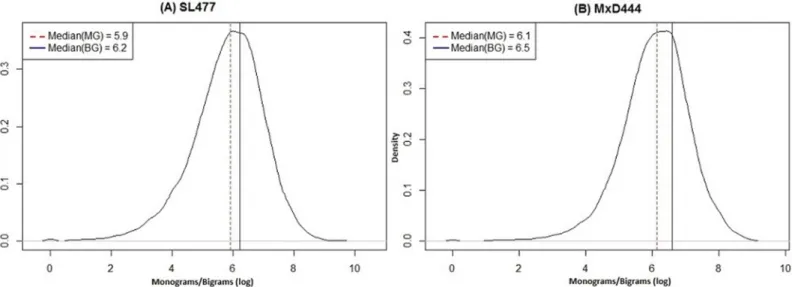
monogram-bigram features are useful in identifying the evolutionary folded (ordered) or, unfolded (disordered) region of proteins, which motivated us to utilize them as features in dis-order prediction. We computed monogram feature matrix (1 × 20) and bigram feature matrix (20 × 20) for each sequence from its PSSM. Monogram feature matrix consists of one mono-gram value (MG) for each type of amino acid and bimono-gram feature matrix consists of one bimono-gram value (BG) for each pair of 20 possible amino acids, respectively. Further, our analysis based on multiple datasets collected from PDB and DisProt shows that both the monograms and bigrams follow a normal density distribution in their logarithmic space with approximately
consistent median value equals to 6.0 within any dataset (Fig 1). Therefore, we used exp(6.0) to
normalize these values and reduce the noise. To distinguish the terminal residues for their posi-tion specific disorder like behavior, we included terminal indicator feature (T) by encoding five
residues of N-terminal as {−1.0,−0.8,−0.6,−0.4,−0.2} and C-terminal as {+1.0, +0.8, +0.6,
+0.4, +0.2} respectively, whereas rest of the residues were labeled 0.0. Note that, we included the fundamental features to characterize disorder in protein in our feature set which are well
studied and utilized in the literature [47]. Further, we enhanced the feature set by including
new features, like MGs and BGs.
Fig 1. Density distribution curves of monograms and bigrams for (A) SL477 and (B) MxD444 dataset.The x-axis and y-axis show the monograms/ bigrams in logarithmic scale and density index of the distribution, respectively. For each figure, the dotted (red) and solid (blue) vertical lines correspond to median values of the distribution for monograms (MG) and bigrams (BG), respectively.
We included the information of neighboring residues within the features of each residue by using a sliding window, keeping the target residue at the center of the window. The motivation was to incorporate the native interactions and contacts of neighboring residues which are found to play essential roles in determining protein structures and protein folding dynamics
[71,72]. We determined the 10-fold cross-validation performance of DisPredict for 13
differ-ent window sizes (1, 3, 5,. . ., 23, 25) to find the optimal window size 21. Thus, there were 1176
(since,window size×total feature count= (21 × 56) = 1176) features used for each residue. The
features were finally scaled within the range [−1, + 1] before using.
2.4 SVM Design and Parameterization
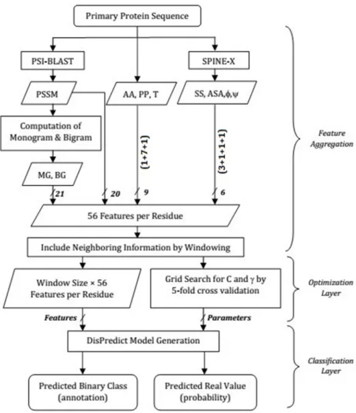
DisPredict is a two-layer disorder predictor that integratesoptimization-layerand
classifica-tion-layer. The classification-layer is developed using a single support vector machine (SVM),
namely LIBSVM [73]. Due to the working principle of SVM of simultaneously minimizing the
empirical classification error (training error) and generalized error (test error) by maximizing the geometric margin of the separating hyperplane, it can be regarded as an effective technique in hard classification problems specially in bioinformatics and computational biology area. We used Gaussian or, radial basis function (RBF) kernel for the SVM to extend its capability to handle non-linearly separable classes. RBF transforms the input feature space into infinite
dimension space (i.e.Hilbert space), which results in a linear separating hyperplane. On the
other hand, in the optimization-layer of DisPredict, we selected two parameters,Candγ,
whereCis the cost of misclassification andγis the parameter of fitting best mode of RBF. The
optimal values for the parametersCandγare determined by grid search using 5 fold cross
vali-dation. However, in our case the grid search turned out to be computationally very intensive. Thus, we used 5% of the training dataset to determine the optimal parameters instead. The Dis-Predict output classes such as disordered or ordered residue, in terms of probability, is opti-mized by another round of 5-fold cross validation. Using the threshold value 0.5, the
probabilities are converted into binary decision variables, where probability ranges 0.5
ran-ged1.0 is considered as disordered and 0.0rangeo<0.5 is considered as ordered.Fig 2
shows the detail paradigm of DisPredict.
We implemented our software in C++. The software is developed and tested on Linux
plat-form. It is dependent on two external packages, namely PSI-BLAST [60] and NR database [27,
64], which are publicly available. DisPredict software is also available online athttps://github.
com/tamjidul/DisPredict_v1.0with a user manual.
2.5 Performance Evaluation and Statistical Test Criteria
The performance of DisPredict is evaluated using the criteria followed in the past Critical
Assessment of protein Structure Prediction (CASP) competitions [74–76]. The measures and
procedures used in CASP experiments are comprehensive. The predictions are done in two levels:
1. Binary value, defining whether a residue is disorder or not (“+1”for disorder and“−1”for
order) and
2. Real value, quantifying the probability of a residue being disorder (“0.5”for disorder and
“<0.5”for order).
Binary prediction evaluation. In binary (two-class) prediction of disorder,TP(True
Posi-tive) = number of correctly predicted disordered residues,TN(True Negative) = number of
disordered residues andFN(False Negative) = number of incorrectly predicted ordered
resi-dues. To determine the total number of correct prediction (both ordered and disordered),N
cor-rect=TP+TNis calculated. Sensitivity(SENS)and specificity(SPEC)are two complementary
statistical measures identifying the proportionate values of correct prediction of disordered (positive class) and ordered (negative class) residues, respectively.
SENS¼ TP TPþFN¼ TP Nd and SPEC¼ TN TNþFP¼ TN No
Here,NdandNoare the total number of disordered and ordered residues, respectively. As
increment of one of these measures (SENS and SPEC) usually leads towards the decrement of another measure, neither of these two measures is a suitable indicator of performance for an
Fig 2. Overview of feature aggregation, optimization-layer and classification-layer in DisPredict.In the feature aggregation step, features are shown in their abbreviated form according toTable 1and the arrows are labeled by the number of features involved. The classification-layer receives final feature set from the feature aggregation step and optimal parameters from the optimization-layer. Then, it generates the predictor model and outputs both binary annotation and real-valued class probabilities.
imbalanced dataset. On the contrary, the balanced accuracy (ACC), weighted score (Sw) and
Mathews correlation coefficient (MCC) are the measures that take all four components of
pre-diction quality (TP, TN, FP and FN) into account and thus can be regarded as more important indicators. ACC¼1 2ð TP TPþFNþ TN TNþFPÞ MCC¼ ffiffiffiffiffiffiffiffiffiffiffiffiffiffiffiffiffiffiffiffiffiffiffiffiffiffiffiffiffiffiffiffiffiffiffiffiffiffiffiffiffiffiffiffiffiffiffiffiffiffiffiffiffiffiffiffiffiffiffiffiffiffiffiffiffiffiffiffiffiffiffiffiffiffiffiffiffiffiffiffiffiffiffiffiffiffiðTPTNÞ ðFPFNÞ ðTPþFPÞðTPþFNÞðTNþFPÞðTNþFNÞ p Sw¼ wdTPwoFPþwoTNwdFN wdNdþwoNo
where,wdis the weight forNd= percentage of ordered residues¼NoNþoNdandwois the weight for
No= percentage of disordered residues¼NoNþdNd[75]. TheSwmeasure includes weight to address
the imbalance in the ratio of ordered and disordered residues and rewards correct disorder
classification over correct classification of ordered residues, which is later found to have a linear
relationship withACC(Sw= 2 ×ACC−1) [77]. Since both of these measures (ACC andSw)
have been used in CASP assessment, we have also included both of them in our paper instead
of just one.MCCscore, another measure that accounts for all four parameters of the prediction
quality, is the most reasonable and consistent measure for disorder prediction assessment
because of not being favorable to over prediction of any class (order/disorder).MCCandSw
scores vary from−1 to 1, where−1 and 1 represent perfect misclassification and classification,
respectively with a random classification scoring by 0. More recently, precision (PPV¼ TP
TPþFP) has been appeared as a good measure for binary disorder prediction as it is totally insensitive to the prediction of the dominant class (i.e., here the order state), is therefore computed to evalu-ate DisPredict. As the prediction becomes better, the values of these metrics also get higher.
We calculated Mean Absolute ErrorðMAEÞ ¼
Pn i¼1jcadðiÞc
p dðiÞj
n to quantify the error of disorder
prediction in content level. Here,nis the total number of protein chains, andcadðiÞandcp
dðiÞare
the actual and predicted disorder content (fraction of disordered residues) for theithprotein
chain, respectively. The lower value of MAE corresponds to better prediction.
Evaluation of predicted probability. The SVM model of DisPredict generates a predicted probability value for each residue which signifies the disorder confidence of that residue. This probability value is then binarized using a threshold of 0.5 to generate class annotation. If the
probability is greater than or equal to 0.5, the predicted class is‘disorder’and if the probability
is less than 0.5, the predicted class is‘order’. Assessment of the predicted probability by a
Dis-Predict is performed by receiver operating characteristic (ROC) curve, which depicts the
corre-lation between the true positive rate (TPRor,SENS) and false positive rate (FPR= 1—SPEC)
for a probability threshold. The area under the ROC curve (AUC) quantifies the predictive
quality of a classifier, where the AUC value equal to 1 indicates a perfect prediction and 0.5 cor-responds to a random prediction. Moreover, 95% confidence interval (CI) for the AUC score is
evaluated using DeLong’s [78] variance estimated by bootstrapping. The evaluation of AUC
and CI are performed using the statistical R package with the pROC [79] library.
3 Test Procedures and Results
3.1 Performance of 10-Fold Cross Validation
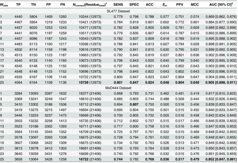
We evaluated the 10-fold cross validation performance of DisPredict separately on SL477 and MxD444 dataset. Regarding the optimum selection of the window size, we ran cross validation
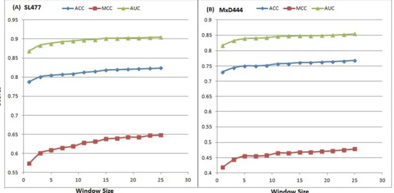
individually for 13 different windows, shown inTable 2, for both of the SL477 and MxD444 dataset with default parameters for SVM. The best result for window size 25 was found with ACC, MCC and AUC values equal to 0.82, 0.65 and 0.91, respectively for SL477 dataset, whereas for MxD444 dataset the values are 0.77, 0.48 and 0.85, respectively. The gradual
increase in performance becomes a plateau as window goes higher above size 23 (Fig 3).
Table 2also depicts the inverse relationship between SENS and SPEC scores with increasing window size for MxD444 dataset. The best SENS (0.74) is achieved by window size 25 while the best SPEC (0.81) is achieved at window size 5. Overall, the consistent increment in balanced accuracy (ACC) and PPV prove our methodology to be well balanced.
Table 2. 10-fold Cross Validation Performance of DisPredict (Default Parameter).
Wsize TP TN FP FN Ncorrect(Residuetotal)
1
SENS SPEC ACC Sw PPV MCC AUC [95% CI]
2 SL477 Dataset 1 4440 5804 1469 1260 10244 (12973) 0.779 0.798 0.788 0.577 0.751 0.574 0.869 [0.862, 0.876] 3 4467 5954 1319 1233 10421 (12973) 0.784 0.819 0.801 0.602 0.772 0.601 0.884 [0.877, 0.890] 5 4457 6020 1253 1243 10477 (12973) 0.782 0.828 0.805 0.609 0.781 0.609 0.889 [0.882, 0.896] 7 4441 6076 1197 1259 10517 (12973) 0.779 0.835 0.807 0.614 0.787 0.615 0.893 [0.886, 0.899] 9 4457 6086 1187 1243 10543 (12973) 0.782 0.837 0.809 0.618 0.789 0.619 0.895 [0.888, 0.902] 11 4483 6113 1160 1217 10596 (12973) 0.786 0.841 0.813 0.627 0.794 0.628 0.898 [0.891, 0.905] 13 4502 6114 1159 1198 10616 (12973) 0.790 0.841 0.815 0.630 0.795 0.631 0.899 [0.892, 0.905] 15 4513 6150 1123 1187 10663 (12973) 0.792 0.845 0.819 0.637 0.801 0.638 0.902 [0.896, 0.909] 17 4540 6133 1140 1160 10673 (12973) 0.796 0.843 0.820 0.640 0.799 0.640 0.902 [0.895, 0.902] 19 4545 6148 1125 1155 10693 (12973) 0.797 0.845 0.821 0.643 0.802 0.643 0.903 [0.896, 0.910] 21 4548 6148 1125 1152 10696 (12973) 0.798 0.845 0.822 0.643 0.802 0.643 0.903 [0.896, 0.910] 23 4555 6167 1106 1145 10722 (12973) 0.800 0.847 0.823 0.647 0.804 0.647 0.904 [0.898, 0.911] 25 4564 6164 1109 1136 10728(12973) 0.801 0.847 0.824 0.648 0.804 0.648 0.905 [0.898, 0.911] MxD444 Dataset 1 3284 13093 3397 1632 16377 (21406) 0.668 0.793 0.731 0.462 0.491 0.419 0.817 [0.810, 0.825] 3 3369 13241 3249 1547 16610 (21406) 0.685 0.803 0.744 0.488 0.509 0.444 0.832 [0.826, 0.840] 5 3410 13302 3188 1506 16712 (21406) 0.694 0.807 0.750 0.500 0.516 0.456 0.839 [0.833, 0.847] 7 3419 13275 3215 1497 16694 (21406) 0.695 0.804 0.750 0.501 0.515 0.455 0.840 [0.833, 0.847] 9 3446 13253 3237 1470 16699 (21406) 0.700 0.805 0.752 0.505 0.516 0.458 0.842 [0.834, 0.849] 11 3503 13232 3258 1413 16735 (21406) 0.712 0.802 0.757 0.515 0.517 0.466 0.846 [0.839, 0.853] 13 3523 13188 3302 1393 16711 (21406) 0.717 0.800 0.758 0.516 0.516 0.466 0.847 [0.839, 0.853] 15 3564 13145 3345 1352 16709 (21406) 0.725 0.797 0.761 0.522 0.515 0.469 0.848 [0.842, 0.855] 17 3578 13097 3393 1338 16675 (21406) 0.728 0.794 0.761 0.522 0.513 0.469 0.848 [0.841, 0.855] 19 3607 13068 3422 1309 16675 (21406) 0.734 0.792 0.763 0.526 0.513 0.471 0.849 [0.842, 0.856] 21 3613 13078 3412 1303 16691 (21406) 0.735 0.793 0.764 0.528 0.514 0.473 0.850 [0.843, 0.857] 23 3640 13059 3431 1276 16699 (21406) 0.740 0.792 0.766 0.532 0.515 0.476 0.851 [0.845, 0.859] 25 3658 13064 3426 1258 16722(21406) 0.744 0.792 0.768 0.536 0.517 0.479 0.852 [0.847, 0.861]
Wsizeindicates the size of sliding window.
Best values of each metric are marked in bold for each dataset separately.
1N
correctis reported with total number of residues (Residuetotal) to be predicted in parentheses. Both of the counts correspond to one subset (fold) of the
full dataset which is generated for performing cross validation.
2For AUC, the values within bracket indicate 95% confidence interval with 2000 stratified bootstrap replicas.
As the window size continues to increase, the rate of increase in scores becomes slow. Increase of scores is0.001, as the windows size grows from 23 to 25 for SL477 dataset and0.004 for MxD444 dataset, respectively.
Note that, this preliminary extensive analysis of performance with multiple window sizes is
done without selection of optimal parameters for SVM. For a specific window size (Wsize) and
total number of residues (Residuetotal) in a dataset, we have a feature matrix of dimension,
Resi-duetotal× (Wsize× 56). Therefore, the increase in window size leads towards the increase in the
dimensions of the feature space, which in turn makes the time expensive grid search for param-eters slower. To trade off between performance with optimization and time complexity of parameter selection along with model generation, we determined the optimal values of parame-ters with a 5% randomly selected subset of residues from training dataset for 3 window sizes
(15, 21 and 25). The optimal parameters (Candγ) found from grid search are reported in
Table 3. Furthermore, we inserted repeated disordered residue information only in case of training to balance the dataset as the support vector points for the less dominant class may not be sufficient to determine the optimal SVM margin. Specifically, duplicates (2 times for SL477 dataset and 3 times for MxD444 dataset) of disorder samples were provided during generation
Fig 3. Increase of performance in 10-fold cross validation (default parameter) according to ACC, MCC and AUC scores with the increase of window size for (A) SL477 and (B) MxD444 dataset.The x-axis and y-axis represent the window sizes and scores, respectively.
doi:10.1371/journal.pone.0141551.g003
Table 3. Optimized Parameters used to build DisPredict Models.
SL477 Dataset MxD444 Dataset
Wsize C γ C γ
15 8.0 0.001953125 8.0 0.0312500
21 2.0 0.007812500 2.0 0.0078125
25 0.5 0.007812500 2.0 0.0078125
Cis the soft penalty parameter to handle overlapped class.
γis the parameter for radial basis kernel for SVM. doi:10.1371/journal.pone.0141551.t003
of predictor model. However, in case of testing, no repeated information was inserted.Table 4
illustrates the detail of the cross validation results with optimized parameters for 3 different window sizes.
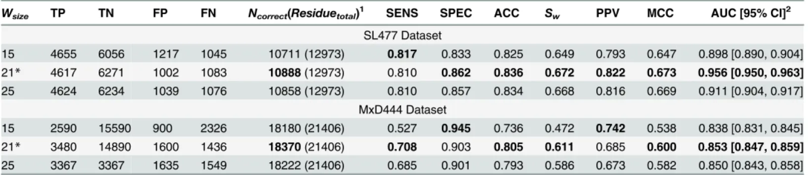
The improvement of performance with optimized parameters over non-optimized one was significant. To compare, for SL477 dataset (window size 21), FP and FN values are reduced to 1,002 and 1,083 from 1,125 and 1,152 due to optimization. In case of MxD dataset (window size 21), the FN value is increased by 133 residues. However, the FP value is also decreased by 1,812 residues which maintains the overall increase in the total number of correctly predicted residues from 16,691 to 18,370. The improvement of prediction, both in terms of increased correct classi-fication and decreased misclassiclassi-fication, is also visible from both the sensitivity and specificity
scores. For window size 21, the values ofSw, precision and MCC are improved by 4.5%, 2.5%
and 4.5% respectively due to optimized training on SL477 dataset. At the same time, for MxD444 dataset, these progresses are 15.7%, 33.3% and 26.8% respectively. Note that, this
sig-nificant improvement in MCC strongly supports our method’s capability in handling the
imbal-ance ratio of ordered and disordered residues. Further, the AUC score is also increased by 4.4% and 0.4% as the result of optimization for SL477 and MxD444 dataset, respectively. A
compara-tive analysis ofTable 2andTable 4also shows that optimized DisPredict model with window
size 21 outperforms all the other models of its own kind. Thus we select 21 as the optimal win-dow size for our proposed DisPredict. Furthermore, to understand the relevance of the new
fea-tures (MGs and BGs) with protein disorder, we separately evaluated optimized DisPredict’s
performance without monograms and bigrams. We performed 10-fold cross validation on SL477 dataset with the optimal window size 21 and optimal parameters of SVM as reported in
Table 3for SL477 dataset with window size 21. The result of this experiment in terms of ACC,
MCC andSwscore are 0.810, 0.651 and 0.621, respectively. The comparison of these scores
excluding MGs and BGs with those of including MGs and BGs (reported inTable 4for SL477
dataset) shows that involvement of MGs and BGs along with PSSM leads to a further increase in binary prediction accuracy in terms of 3.2% improved ACC (0.810 to 0.836), 3.8% improved
MCC (0.651 to 0.673) and 8.2% improvedSwscore (0.621 to 0.672).
To uniformly distribute the residues into ten subsets for cross validation, we applied modu-lar arithmetic operation to split the dataset in residue level. As the residues are already included within the neighboring information based on the window, they are detachable from their
Table 4. 10-fold Cross Validation Performance of DisPredict (Optimized Parameter).
Wsize TP TN FP FN Ncorrect(Residuetotal)
1
SENS SPEC ACC Sw PPV MCC AUC [95% CI]
2 SL477 Dataset 15 4655 6056 1217 1045 10711 (12973) 0.817 0.833 0.825 0.649 0.793 0.647 0.898 [0.890, 0.904] 21* 4617 6271 1002 1083 10888(12973) 0.810 0.862 0.836 0.672 0.822 0.673 0.956 [0.950, 0.963] 25 4624 6234 1039 1076 10858 (12973) 0.810 0.857 0.834 0.668 0.816 0.669 0.911 [0.904, 0.917] MxD444 Dataset 15 2590 15590 900 2326 18180 (21406) 0.527 0.945 0.736 0.472 0.742 0.538 0.838 [0.831, 0.845] 21* 3480 14890 1600 1436 18370(21406) 0.708 0.903 0.805 0.611 0.685 0.600 0.853 [0.847, 0.859] 25 3367 3367 1635 1549 18222 (21406) 0.685 0.901 0.793 0.586 0.673 0.582 0.850 [0.843, 0.858]
Wsizeindicates the size of sliding window and*mark represents window size with overall optimal (best) performance. Best values of each metric are marked in bold for each dataset separately.
1N
correctis reported with total number of residues (Residuetotal) to be predicted in parentheses. Both of the counts correspond to one subset (fold) of the
full dataset which is generated for performing cross validation.
2For AUC, the values within bracket indicate 95% confidence interval with 2000 stratified bootstrap replicas.
original sequence. However, this inclusion of residue information within window may yield overlap of information between training and test sets in case of residue level splitting of dataset for cross validation. We analyzed the probability of this residual overlap between training and
test sets. Let, there areNsequences in the dataset and the expected length of the sequence isL.
Then, the possibility of picking two residues for training and test subsets of 10 fold cross
valida-tion which belongs to same sequence isð9N1
10
1
N 10Þ ¼
100
9N2. Since the expected length of a sequence
isL, the chance of training and test overlap for a specific window size (Wsize) isWsizeL1.
Alto-gether, the probability of a train and test residue overlap from the same sequence is ð100
9N2 Wsize1
L Þ ¼ ð1009Þ
Wsize1
N2L . For SL477 dataset withN= 477, approximateL¼400andWsize=
21, the probability of the overlap is 2.44 × 10−06, which is significantly low and thus can be
safely ignored. Further, we reevaluated DisPredict’s 10 fold cross validation performance with
sequence level sampling by modular operation for SL477 dataset to generate training and test
subsets.Table 5quantifies the difference in performance between residue level and state of the
art practice of sequence level splitting of dataset for cross validation with window size 21 and
default parameters for SVM. It justifies that DisPredict’s performance remains consistent
with-out any significant over prediction in terms of all the metrics.
3.2 Evaluation of Independent Training and Testing
With optimized parameters and balanced dataset, we carried out independent training on SL477 and MxD444 datasets followed by testing the resulting predictor model with MxD134 and SL171 dataset, respectively. Note that, these independent test datasets (MxD134 and SL171) were generated at low sequence identity (10%) with the corresponding training datasets (SL477 and MxD444). The consistent results of these two tests done through cross validation and independent test confirm the usage of robust technique and effective feature set in
DisPre-dict as well as training efficacy avoiding possible over-fittings.Table 6further illustrates the
Table 5. DisPredict’s cross validation performance with residue level and sequence level splitting of SL477 dataset.
Splitting Method SENS SPEC ACC Sw PPV MCC AUC [95% CI] Residue Level 0.798 0.845 0.822 0.643 0.802 0.643 0.903 [0.896, 0.910] Sequence Level 0.784 0.844 0.814 0.628 0.793 0.627 0.892 [0.886, 0.898]
Default values ofCandγare applied for SVM. Window size 21 is used.
doi:10.1371/journal.pone.0141551.t005
Table 6. Performance Comparison of Cross Validation and Independent Tests. Model Evaluation Procedure1 SENS (STDEV) SPEC (STDEV) ACC (STDEV) Sw(STDEV) PPV (STDEV) MCC (STDEV) AUC (STDEV) MAE (STDEV)
10-fold cross validation on SL477
0.810 (0.004) 0.862 (0.001) 0.836 (0.002) 0.672 (0.005) 0.822 (0.002) 0.673 (0.004) 0.956 (0.007) 0.032 (0.002)
Train by SL477, Test on MxD134
0.744 (0.002) 0.923 (0.002) 0.833 (0.002) 0.667 (0.003) 0.574 (0.002) 0.598 (0.004) 0.906 (0.001) 0.023 (0.001)
10-fold cross validation on MxD444
0.708 (0.006) 0.903 (0.001) 0.805 (0.003) 0.611 (0.006) 0.685 (0.002) 0.600 (0.004) 0.853 (0.007) 0.208 (0.001)
Train by MxD444, Test on SL171
0.718 (0.003) 0.860 (0.001) 0.789 (0.001) 0.577 (0.003) 0.748 (0.003) 0.583 (0.002) 0.872 (0.007) 0.151 (0.001)
1All the evaluations are carried out using a sliding window of length 21 and optimized parameters for SVM.
results of these tests, where we reported the average of the scores computed for equally divided 10 subsets of the full dataset along with the corresponding standard deviation (STDEV).
Table 6reveals that training by SL477 dataset gives consistent performance regardless of test datasets and test procedures (cross validation or independent test) in terms of ACC: 0.836,
0.833 andSw: 0.672, 0.667. These consistencies are also evident in case of training with
MxD444 dataset while tested by different datasets and the evaluations are, ACC: 0.805, 0.789
andSw: 0.611, 0.577. We calculated the Mean Absolute Error (MAE) which is also reported
along with its corresponding STDEV from mean. The score indicates that the error does not increase from cross validation to independent test as the test-results were robust.
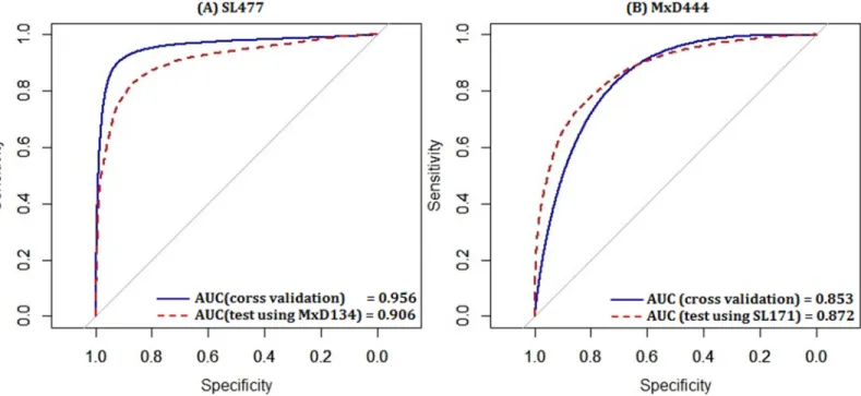
To analyze the probability prediction, the ROC curves given by DisPredict are plotted inFig
4in continuous scale between 0.0 and 1.0. In each figure, two ROCs are plotted keeping the
training dataset same with varying test datasets and evaluation procedure. Finally, we reported the AUC values which are found consistent for cross validation and independent test indicating
our predictor’s capability to avoid over-fitting.
3.3 Comparison with Existing Predictors
The performance of DisPredict is compared with the state-of-the-art disorder predictors,
MFDp [56] and SPINE-D [47]. To remain fair while comparing DisPredict with each of the
above two predictors, we train DisPredict separately with respective datasets and compare with each of them separately. Thus, DisPredict is compared with MFDp based on dataset MxD444,
while dataset SL477 is used to compare DisPredict with SPINE-D (Table 7).
In particular, MFDp [56] is a meta predictor that combines the predictions from three
dis-order predictors (DISOPRED2 [32], IUPred [50] and DISOclust [53]). Further, MFDp
com-bines the outputs from three SVMs with linear kernel using a threshold of 0.37, used to output
Fig 4. ROC curves given by DisPredict for the probability prediction per residue while the training is performed with (A) SL477 and (B) MxD444 dataset.In each figure, the solid (blue) curve corresponds to the cross validation test on the same dataset and the dotted (red) curve corresponds to the independent test. The AUC values given in each figure correspond to the values inTable 6. The x-axis and y-axis show the Specificity and Sensitivity, respectively.
binary prediction. In contrast, we utilized single SVM with RBF kernel and optimized parame-ters combined with a comprehensive set of features to develop the standalone predictor.
How-ever, the performance of MFDp inTable 7is of 5-fold cross validation whereas DisPredict is
evaluated by 10-fold cross validation and hence to be considered reliable rather than over-fitted by chance. In terms of MCC, DisPredict improved significantly, which is 36.36% better than
MFDp. The improvement inSwscore is also 19.6%. DisPredict showed lower sensitivity (7%)
than MFDp while at the same time improved specificity by 20%, which in turn improved the balanced accuracy by 6.67%. Moreover, DisPredict outperformed MFDp in AUC score by 1.29% which is used to assess the probability based prediction.
The other state of the art predictor, SPINE-D [47] utilizes ANN technique which was at first
developed to output three state prediction and later reduced into two state predictor of ordered and disordered residues. SPINE-D employs a disorder probability threshold of 0.06 that was
optimized to achieve maximum Swscore. On the contrary, DisPredict is a SVM based two state
disorder predictor using a more meaningful threshold for two-class classification of value 0.5. DisPredict outperformed SPINE-D in terms of sensitivity as well as specificity by 5.19% and 1.18% respectively which leads to 3.7% improvement in overall accuracy. DisPredict also
out-performed SPINE-D in terms of Sw, MCC and AUC by 8.06%, 6.34% and 10.34% respectively.
In addition to the comparison on cross validation test, we evaluated DisPredict, SPINE-D
[47] and MFDp [56] on independent DD73 dataset. The comparison among these three
meth-ods is illustrated inTable 8. It shows that DisPredict gives better performance among three
pre-dictors except in case of sensitivity. DisPredict yielded 2.63% lower sensitivity than that of
SPINE-D [47], whereas DisPredict gave 4.25% higher specificity than that of SPINE-D [47].
Table 8also shows that DisPredict outperformed SPINE-D [47] and MFDp [56] in terms of MCC by 3.76% and 0.76%, respectively. At the same time, DisPredict gave 1.26% and 5.36%
improved precision (PPV) than MFDp [56] and SPINE-D [47], respectively. However,
Table 7. Comparative predictive quality of DisPredict with MFDp on MxD444 dataset and SPINE-D on SL477 dataset.
Method SENS SPEC ACC Sw MCC AUC
DisPredict2 0.71 0.90 0.80 0.61 0.60 0.85
MFDp1 0.76 0.75 0.75 0.51 0.44 0.81
DisPredict3 0.81 0.86 0.84 0.67 0.67 0.96
SPINE-D4 0.77 0.85 0.81 0.62 0.63 0.87
15-fold cross validation performance of MFDp on MxD dataset of 514 protein chains [56].
210-fold cross validation performance of DisPredict on MxD444 which is a subset of 444 chains out of 514 chains with no X-tag. 310-fold cross validation performance of DisPredict on SL477.
410-fold cross validation performance of SPINE-D [47] on SL477.
doi:10.1371/journal.pone.0141551.t007
Table 8. Performane comparison among DisPredict, SPINE-D and MFDp on independent DD73 dataset.
Predictor SENS SPEC ACC Sw PPV MCC AUC [95% CI]
DisPredict* 0.775 0.883 0.829 0.658 0.806 0.663 0.89 [0.88, 0.90]
SPINE-D 0.796 0.847 0.822 0.644 0.765 0.639 0.89 [0.88, 0.90]
MFDp 0.780 0.875 0.828 0.656 0.796 0.658 0.88 [0.87, 0.89]
Best results are marked in bold.
*Window size = 21,C= 2.0 andγ= 0.0078125. doi:10.1371/journal.pone.0141551.t008
DisPredict resulted slightly lower sensitivity than those of SPINE-D [47] and MFDp [56]. At
the same time, both SPINE-D [47] and MFDp [56] gave lower specificity than that of
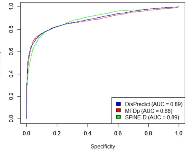
DisPre-dict. Figs5and6compare the ROC curves and precision-recall curves, respectively, given by
DisPredict, SPINE-D [47] and MFDp [56].Fig 5shows that the ROC curves given by the three
predictors are comparative. At the same time, the precision-recall curves (Fig 6) depicts that
DisPredict achieves consistently higher precision upto less than 65% sensitivity (recall). MFDp and SPINE-D have been established as the best disorder predictor among 8 and 11
existing disorder predictors [47,56], respectively, covering different approaches in their
rele-vant publication. In this article, our predictor is shown to be comparable with both of these methods. Therefore, DisPredict can be considered to be one of the finest disorder predictor and can be utilized to produce more reliable annotation of disorder versus order residues.
3.4 Case Studies: Characteristic Region and Protein Function
Proteins with disordered regions are found to contain several regions of interest, such as self-stabilizing folded regions, DNA or, nucleotide binding regions, short (up to 20 amino acids) conserved regions of biological significance (known as motif), mediating regions for protein interaction with different partners etc. These characteristic regions undergo various conforma-tional changes, gain structure and affect many important biological functions. We selected three proteins as cases (UniProt IDs: P41212, P01116 and P04637) with experimentally verified
Fig 5. ROC curves for disorder prediction on DD73 dataset given by DisPredict(blue), SPINE-D(green) and MFDp(red).The AUC values shown in the figure correspond to the values inTable 8. The x-axis and y-axis show the Specificity and Sensitivity, respectively.
regions of interest to analyze per residue disorder confidence score assigned by DisPredict,
SPINE-D and MFDp.Fig 7illustrates the disorder probability of each residue with respect to
residue index. P41212 (Fig 7(A)) is a human ETV6 protein for transcriptional repressor
func-tion, which is also involved in several kinds of leukemia and syndrome. For this protein, Dis-Predict and SPINE-D showed comparable performance in detecting the highly conserved
region of PNT (pointed) domain [80] [residues 40−124] and ETS (E26
transformation-spe-cific) DNA binding region [81] [residues 339−420], respectively, while MFDp outperformed
both of them with relatively less noise. P01116 (Fig 7(B)) is a human KRAS protein with
intrin-sic GTPase activity (binds GDP/GTP [82]) and related to several diseases, such as gastric
can-cer (GASC), acute myelogenous leukemia (AML), cardiofaciocutaneous syndrome 2 (CFC2) etc. DisPredict could identify its GTP (guanosine triphosphate) binding region [residues 10
−17] and effector region [residues 32−40] respectively, with close to cut-off (0.5) probabilities.
Note that, these two regions are experimentally verified unstructured regions, which are strongly suggested as structured by both SPINE-D and MFDp. However, the C-terminal
hyper-variable region [residues 166−185] is consistently detected by all three of these predictors.
P04637 corresponds to human p53 protein which acts as a tumor suppressor.Fig 7(C)
illus-trates that DisPredict and MFDp outperformed SPINE-D with relatively sharp detection of
N-terminal TADI (transcriptional repression domain-I) motif [83] [residues 17−25]. On the
other hand, DisPredict and SPINE-D outperformed MFDp in determining oligomerization
Fig 6. Precision-Recall curves for disorder prediction on DD73 dataset given by DisPredict(blue), SPINE-D(green) and MFDp(red).The x-axis and y-axis show the Recall(Sensitivity) and Precision (PPV), respectively.
Fig 7. Disorder probability plot for (A) human ETV6 (P41212), (B) human KRAS (P01116) and (C) human p53 (P04637) proteins, given by DisPredict (red), SPINE-D (blue) and MFDp (green).In (P41212, A), the yellow (40−124 residues) and pink bar (339−420 residues) represent to the PNT domain [80] and ETS DNA binding region [81], respectively. In (P01116, B), the orange (10−17 residues), cyan (32−40 residues) and purple bar (166−185 residues) correspond to the GTP binding region [82], effector region and hypervariable region, respectively. In (P04637, C), the dark green (17−25 residues), red (325−356 residues) and gray bar (370−372 residues) highlight to the TADI motif [83], oligomer region and [KR]-[STA]-K binding motif, respectively.
domain [84] of residues 325−356.Fig 7(C)also shows that both SPINE-D and MFDp missed
the very short, 3 residue (370−372) long [KR]-[STA]-K binding motif at C-terminal, while
DisPredict detected it correctly. The overall comparison depicts that DisPredict’s performance
is more biologically relevant with correct identification of these short regions. Therefore, it would be interesting to utilize DisPredict in a broader scope in near future.
4 Discussion
In this article, we proposed a canonical support vector machine which uses a RBF kernel and includes useful and advanced features for predicting disordered residues, called DisPredict. Dis-Predict not only generates the binary class annotation for ordered and disordered residues but also provides order-disorder probabilities that can be treated as the confidence level of the diction too. The DisPredict outperforms other existing top performing predictors both in pre-dicting binary annotation and probability. The competitive performance of DisPredict is mainly due to the use of a novel methodology that incorporates firstly, radial basis kernel function (RBF) that can implicitly map the feature space in infinite dimension, secondly and most impor-tantly the optimization of the parameters and thirdly, the novel features monogram (MG) and bigram (BG) assisted in determining an optimal as well as effective class separating hyperplane.
This overall performance of DisPredict is also persuaded by the use of a comprehensive set of features that well captures the sequential (amino acid composition) and structural
character-ization of ordered and disordered residues or, proteins. We used SPINE X [65] to generate the
secondary structure related fine features. The distinguishing property of our feature set in parison with existing predictors is the inclusion of monogram (MG) and bigram (BG), com-puted from PSSM. When a region of a protein is evolutionary conserved in a fold, then all the proteins within that fold are likely to have a conserved group of MGs and BGs. As some intrin-sic disordered regions are conserved, addition of these features provides important structural evolutionary characteristics. By determining the appropriate window size, we have also included the effect of optimal interactions due to the contacts among neighboring residues.
The robust performance of DisPredict is also justified by training and testing the predictor with multiple datasets: SL477, SL171 and MxD444, MxD134. The datasets used to train DisPre-dict encompass disorder annotation from several complementary sources (X-ray and NMR defined disorder from PDB and DisProt) as well as disorder region of various lengths. The SL dataset comprises of 81 full disordered proteins (IDPs) while the rest of the chains contain 928 disordered regions (IDRs). On the other hand, the MxD dataset is composed of 55 full disor-dered chains, 4 full ordisor-dered chains and 385 chains, sharing both structured and disordisor-dered regions, which include 730 disordered regions (IDRs). Furthermore, 70% of the IDRs included
within partially disordered proteins are short (30 residues) and 30% of them are long (>30
residues). This combination of several length disordered regions (Fig 8) included within
train-ing confirms the consistent performance of DisPredict for disordered regions of all sizes as well as different types of disordered residues.
It is interesting to note that, regardless of cross validation or independent test, DisPredict’s
performance is relatively better while it is trained on SL477 dataset than that of MxD444 (Table 6). To further insight into this discrepancy, we investigated the correlation of true anno-tation provided in the dataset with the actual structural characterization of disordered and ordered residues. Disordered residues are distinguished from ordered residues by low content
of secondary structure [8,28], therefore high probability of coil residues than helical or beta
strand residues and disordered regions are likely to have large solvent accessible (exposed) area
[55]. We represented the correlation of the fraction of secondary structure content and fraction
predicted probability of each residue to be coil and predicted per residue solvent accessibility
provided by SPINE-X [65] since all residues do not have defined coordinates (structure) to
compute secondary structure and solvent accessibility.
We calculated the average coil probability (Pcoil) for each ordered or disordered region and
computed the fraction of exposed residues with greater than 25% solvent accessibility (Fexposed)
of that region. In this analysis, we discarded 5 residues from N and C-terminal regions of each
Fig 8. Distribution of disordered regions of different lengths in MxD444 (left) and SL477 (right) dataset.Legends are shown for different range of lengths (with interval size 15) and each bar is labeled with total number of occurrence of a disordered region of this specific length.
doi:10.1371/journal.pone.0141551.g008
Fig 9. Correlation plot between structural characterizations of ordered (blue) and disordered (red) regions within (A) SL477 and (B) MxD444 dataset.The x-axis and y-axis correspond to the probability of having well defined secondary structure (in terms of probability being coil) and fraction of exposed residues of that region, respectively.
protein sequence as they are mostly found on the surface of a protein chain (not buried in the core) and more likely to be affected by the interaction with nearby structured protein, yielding to a highly flexible and dynamic conformation. The plots for both datasets show that the ordered regions are mostly concentrated in the portion with relatively low coil probability, 0.3
Pcoil<0.5 (high content of well defined helical or strand secondary structured residues) and
low exposure, 0.2Fexposed<0.5. While on the contrary, the disorder regions are found
abun-dant in the area of high coil probability, 0.5Pcoil0.9 (low content of helical or strand
sec-ondary structured residues) and high exposure, 0.5Fexposed1.0. However, we found the
intrinsic difference between these two datasets according to their annotation of residues as order and disorder. This difference is also evident from the top right location of the correlation
plot, 0.6Pcoil0.8 and 0.4Pcoil0.9, designated for disordered regions. For SL477
data-set (Fig 9(A)), the number disordered regions are predominant over the number of ordered
regions in this top right location of disordered regions in the plot. In contrast, the same loca-tion of the plot is overlapped by both ordered and disordered regions in case of MxD444. We
further quantified the difference as 13% of the data in MxD444’s ordered set are more likely to
be coil as well as highly exposed while 6% of the data in SL477’s ordered set are exposed as well
as coil. This higher proportion of misleading annotation in MxD444 dataset contributes rela-tively lower signal to noise ratio (SNR) of 87/13 compared to 94/6 for SL477 which is the most compelling reason of the better performance of DisPredict in case of training dataset SL477 over MxD444. As the prediction produced by DisPredict is well capable of detecting such dis-crepancies in the native annotation of the datasets, it can be utilized as a reliable source of cor-rect annotation of the ordered and disordered residues. We should also focus that, a similar proportion of 11% and 13% of the disordered data are also mixed with the ordered residues in the low coil probability region of the plot for both MxD444 and SL477 dataset, respectively.
We would like to highlight that the amino acid residue compositions may vary in different
datasets as well as within short (30 residues) and long (>30 residues) disordered regions
[28,29]. Specifically, short disordered regions are enriched with aspartic acid (D), glycine (G)
and serine (S). On the contrary, glutamic acid (E), lysine (K) and proline (P) are likely to be abundant in long disordered regions. To give further insight into this residue composition and confirm the ability of DisPredict to detect the residue preferences of short and long disordered
regions, we determined the residual composition profile for our two test datasets, SL171 (Fig
10(A)) and MxD134 (Fig 10(B)). It is to be noted that, these two datasets contain experimen-tally annotated disorder from two different sources. SL171 contains sequences with disorder
Fig 10. Percentage of amino acid type residues in actual composition (blue, or left adjacent bar) and predicted composition (red, or right adjacent bar) of (A) SL171 and (B) MxD134 dataset.Thex-axis andy-axis represent the 20 different amino acids and their relative proportions in the composition. doi:10.1371/journal.pone.0141551.g010
annotation from DisProt while MxD134 contains that from PDB. The composition profile
con-sists of the actual ratio (ra) and predicted ratio (rp) of each amino acid type out of total
anno-tated and predicted disordered residues.
The composition profile demonstrates that SL171’s disordered residue set accommodates
relatively higher ratio of amino acid type E (10%) and K (9%), which are long disorder prone
residues. In contrast, MxD134’s disordered residue set is enriched with high ratio of amino
acid type S (11%), G (10%) and D (9%), known as short disorder prone residues. Another sig-nificant difference between the intrinsic compositions of these two datasets is in the proportion of histidine (H). Disorder annotation from PDB includes higher ratio of H-tag (8% in
MxD134, compared to 2% in SL171), which is sometimes used for protein purification. The predicted proportion of all these amino acids given by DisPredict ensures its capability of detecting residues in disordered region of all length accurately with no significant over predic-tion. Moreover, DisPredict could also accurately predict methionine (M) at highly flexible
N-terminal region. To further quantify DisPredict’s performance in detecting residue
composi-tion, we evaluated the Root Mean Square Difference (RMSE) and Pearson Correlation
Coeffi-cient (PCC) between actual and predicted ratio (raandrp) for each amino acid type. For
MxD134 test dataset, we found RMSE of 0.0046, which was comparatively higher than the RMSE value computed for SL171 which equals to 0.0018. However, the correspondence between actual composition and predicted composition by DisPredict measured with PCC
(P-Value<10−5) was found equally positive, 0.9976 and 0.9897 for SL171 and MxD134
data-set, respectively. It is important to note that, this consistent result is corresponding to the inde-pendent test where the dataset used to train DisPredict shared significantly low sequence identity (at most 10%) with test dataset, which once again implicates the strength of the classifi-cation methodology of DisPredict.
Finally, accurate prediction of disorder has useful implication in proteomic studies due to its direct involvement in the proper function of a protein. Successful detection of disordered region of a protein is considered to be the first step in drug design to combat critical diseases. We have built DisPredict using the canonical SVM classifier with RBF kernel and established it as a successful fine predictor of disorder by utilizing the benchmark datasets. In addition to that, our case studies ensure biologically relevant performances of DisPredict.
Acknowledgments
We gratefully acknowledge the Louisiana Board of Regents through the Board of Regents
Sup-port Fund, LEQSF (2013–16)-RD-A-19. We also acknowledge the discussion with Md Nasrul
Islam, Avdesh Mishra and Denson Smith. Special thanks to Denson Smith for critically review-ing the paper.
Author Contributions
Conceived and designed the experiments: SI MTH. Performed the experiments: SI. Analyzed the data: SI MTH. Contributed reagents/materials/analysis tools: SI MTH. Wrote the paper: SI MTH.
References
1. Wright PE, Dyson HJ. Intrinsically unstructured proteins: re-assessing the protein structure-function paradigm. Journal of Molecular Biology. 1999; 293: 321–331. doi:10.1006/jmbi.1999.3110PMID: 10550212
2. Uversky VN, Dunker AK. Understanding protein non-folding. Biochimica Et Biophysica Acta (BBA)— Proteins And Proteomics. 2010; 1804: 1231–1264. doi:10.1016/j.bbapap.2010.01.017
3. Uversky VN, Gillespie JR, Fink AL. Why are“natively unfolded”proteins unstructured under physiologic conditions? Proteins. 2000; 41: 415–427. doi: 10.1002/1097-0134(20001115)41:3%3C415::AID-PROT130%3E3.3.CO;2-ZPMID:11025552
4. Uversky VN. Natively unfolded proteins: A point where biology waits for physics. Protein Science. 2002; 11: 739–756. doi:10.1110/ps.4210102PMID:11910019
5. Tompa P. Intrinsically unstructured proteins. TRENDS in Biochemical Sciences. 2002; 10: 527–533. doi:10.1016/S0968-0004(02)02169-2
6. Dunker AK, Obradovic Z. The protein trinity–linking function and disorder. Nat Biotechnol. 2001; 19: 805–806. doi:10.1038/nbt0901-805PMID:11533628
7. Vucetic S, Brown CJ, Dunker AK, Obradovic Z. Flavors of protein disorder. Proteins: Structure, Func-tion, Bioinformatics. 2003; 52: 573–584. doi:10.1002/prot.10437
8. Radivojac P, Iakoucheva LM, Oldfield CJ, Obradovic Z, Uversky VN, Dunker AK. Intrinsic Disorder and Functional Proteomics. Biophysical Journal. 2007; 92: 1493–1456. doi:10.1529/biophysj.106.094045
9. Whitford PC. Disorder guides protein function. Proc Natl Acad Sci USA. 2013; 110: 7114–7115. doi:10. 1073/pnas.1305236110PMID:23610426
10. Dyson HJ, Wright PE. Coupling of folding and binding for unstructured proteins. Current opinion in structural biology. 2002; 12: 54–60. doi:10.1016/S0959-440X(02)00289-0PMID:11839490
11. Uversky VN, Oldfield CJ, Dunker AK. Showing your ID: intrinsic disorder as an ID for recognition, regu-lation, cell signaling. J. Mol. Recogn. 2005; 18: 343–384. doi:10.1002/jmr.747
12. Dunker AK, Brown CJ, Obradovic Z. Identification and functions of usefully disordered proteins. Adv. Protein Chem. 2002; 62: 25–49. doi:10.1016/S0065-3233(02)62004-2PMID:12418100
13. Dunker AK, Brown CJ, Lawson JD, Iakoucheva LM, Obradovic Z. Intrinsic disorder and protein function. Biochemistry. 2002; 41: 6573–6582. doi:10.1021/bi012159+PMID:12022860
14. Xue B, Dunker AK, Uversky VN. The Roles of Intrinsic Disorder in Orchestrating the Wnt-Pathway. Journal of Biomolecular Structure and Dynamics. 2012; 29: 843–861. doi:10.1080/
073911012010525024PMID:22292947
15. Kulkarni P, Rajagopalan K, Yeater D, Getzenberg RH. Protein folding and the order/disorder paradox. J Cell Biochem. 2011; 112: 1949–1952. doi:10.1002/jcb.23115PMID:21445877
16. Uversky VN, Oldfield CJ, Midic U, Xie H, Xue B, Vucetic S, et al. Unfoldomics of human diseases: link-ing protein intrinsic disorder with diseases. BMC Genomics. 2009; 10: S1–S7. doi: 10.1186/1471-2164-10-S1-S7
17. Babu MM, Lee R, Groot NS, Gsponer J. Intrinsically disordered proteins: regulation and disease. Cur-rent Opinion in Structural Biology. 2011; 21: 432–440. doi:10.1016/j.sbi.2011.03.011PMID:21514144
18. Cheng Y, LeGall T, Oldfield CJ, Mueller JP, Van Y-YJ, Romero P, et al. Rational drug design via intrinsi-cally disordered protein. Trends Biotechnol. 2006; 24: 435–442. doi:10.1016/j.tibtech.2006.07.005 PMID:16876893
19. Berman HM, Westbrook J, Feng Z, Gilliland G, Bhat TN, Weissig H, et al. The Protein Data Bank. Nucleic Acids Res. 1999; 28: 235–242. doi:10.1093/nar/28.1.235
20. Obradovic Z, Peng K, Vucetic S, Radivojac P, Brown CJ, Dunker AK. Predicting intrinsic disorder from amino acid sequence. Proteins. 2003; 53: 566–572. doi:10.1002/prot.10532PMID:14579347
21. Xue B, Dunbrack RL, Williams RW, Dunker AK, Uversky VN. PONDR-FIT: A Meta-Predictor of Intrinsi-cally Disordered Amino Acids. Biochim Biophys Acta. 2010; 1804: 996–101. doi:10.1016/j.bbapap. 2010.01.011PMID:20100603
22. Sickmeier M, Hamilton JA, LeGall T, Vacic V, Cortese MS, Tantos A, et al. DisProt: the Database of Dis-ordered Proteins. Nucleic Acids Res. 2007; 35: 786–793. doi:10.1093/nar/gkl893
23. Fukuchi S, Amemiya T, Sakamoto S, Nobe Y, Hosoda K, Kado Y, et al. IDEAL in 2014 illustrates inter-action networks composed of intrinsically disordered proteins and their binding partners. Nucleic Acids Res. 2014; 42: D320–D325. doi:10.1093/nar/gkt1010PMID:24178034
24. Fukuchi S, Sakamoto S, Nobe Y, Murakami SD, Amemiya T, Hosoda K, et al. IDEAL: Intrinsically Disor-dered proteins with Extensive Annotations and Literature. Nucleic Acids Res. 2012; 40: D507–D511. doi:10.1093/nar/gkr884PMID:22067451
25. Potenza E, Domenico TD, Walsh I, Tosatto SCE. MobiDB 2.0: an improved database of intrinsically dis-ordered and mobile proteins. Nucl. Acids Res. 2014; 43: D315–D320. doi:10.1093/nar/gku982PMID: 25361972
26. Domenico TD, Walsh I, Martin AJM, Tosatto SCE. MobiDB: a comprehensive database of intrinsic pro-tein disorder annotations. Bioinformatics. 2012; 28(15): 2080–2081. doi:10.1093/bioinformatics/bts327 PMID:22661649