Border Feature Detection And Adaptation: A New Algorithm For Classification Of Remote Sensing Images

İSTANBUL TECHNICAL UNIVERSITY  INSTITUTE OF SCIENCE AND TECHNOLOGY

Ph.D. Thesis by

N. Gökhan KASAPOĞLU, M.Sc.

Department : Electronics and Communication Engineering

Programme: Electronics and Communication Engineering

MAY 2007

BORDER FEATURE DETECTION AND ADAPTATION: A NEW ALGORITHM FOR CLASSIFICATION OF

İSTANBUL TECHNICAL UNIVERSITY  INSTITUTE OF SCIENCE AND TECHNOLOGY

Ph.D. Thesis by

N. Gökhan KASAPOĞLU, M.Sc. (504002207)

Supervisors (Chairmen): Prof. Dr. Bingül YAZGAN

Prof. Dr. Okan K. ERSOY (Purdue) Members of the Examining Committee Prof. Dr. Ahmet H. KAYRAN (İTÜ)

Prof. Dr. Osman N. UÇAN (İÜ) Prof. Dr. Aydın AKAN (İÜ) Prof. Dr. Metin YÜCEL (YTÜ)

Assoc. Prof. Dr. Sedef KENT (İTÜ) BORDER FEATURE DETECTION AND ADAPTATION:

A NEW ALGORITHM FOR CLASSIFICATION OF REMOTE SENSING IMAGES

MAY 2007

Date of submission : 8 February 2007 Date of defence examination : 25 May 2007

İSTANBUL TEKNİK ÜNİVERSİTESݐ FEN BİLİMLERİ ENSTİTÜSÜ

SINIR ÖZNİTELİKLERİNİN BELİRLENMESİ VE ADAPTASYONU: UZAKTAN ALGILAMA GÖRÜNTÜLERİNİN SINIFLANDIRILMASI İÇİN

YENİ BİR ALGORİTMA

DOKTORA TEZİ

Y. Müh. N. Gökhan KASAPOĞLU (504002207)

MAYIS 2007

Tezin Enstitüye Verildiği Tarih : 8 Şubat 2007 Tezin Savunulduğu Tarih : 25 Mayıs 2007

Tez Danışmanları: Prof. Dr. Bingül YAZGAN

Prof. Dr. Okan K. ERSOY (Purdue) Diğer Jüri Üyeleri Prof. Dr. Ahmet H. KAYRAN (İTÜ)

Prof. Dr. Osman N. UÇAN (İÜ) Prof. Dr. Aydın AKAN (İÜ) Prof. Dr. Metin YÜCEL (YTÜ)

PREFACE

I would like to express my gratitude to my advisor Prof. Dr. Okan K. Ersoy for his guidance and reviewing my thesis. Without his constant support this thesis would not materialize.

I would like to express my special thanks to my advisor, Prof. Dr. Bingül Yazgan and steering committee members; Prof. Dr. Ahmet H. Kayran and Prof. Dr. Osman N. Uçan for their support.

AVIRIS and Landsat data used in chapter 5 were obtained from Purdue LARS (Laboratory for Applications of Remote Sensing) and GLCF (Global Land Cover Facility) respectively. Therefore, I would like to thank both LARS and GLCF for sharing their data resources.

My family has always encouraged me during my Ph.D. study. I appreciate to my mother Nimet Kasapoğlu, my sister Nurgül Kınacı and my nephew, Yarkın Kınacı

for their support and patience. At last, I wish to dedicate this thesis to my father, Mehmet Kasapoğlu.

TABLE OF CONTENTS

LIST OF ABBREVIATIONS vi

LIST OF TABLES vii

LIST OF FIGURES viii

ÖZET ix SUMMARY xii

1. INTRODUCTION 1

1.1. Multispectral and Hyperspectral Data Structure 1

1.2. General Classification Problem 4

1.3. Problem Description and Aims of This Thesis 4

1.4. Organization of the Thesis 7

2. FEATURE EXTRACTION 8

2.1. Methods for Feature Dimension Reduction 9

2.1.1. Dimension Reduction via Projection Pursuit (PP) 11

2.2. Spatial Feature Extraction 15

3. TYPES OF CLASSIFIERS 17

3.1. Statistical Classifiers 18

3.1.1. Maximum Likelihood Classifier 18

3.1.2. Expectation Maximization (EM) 21

3.2. Nonparametric Methods 23

3.2.1. K-Nearest Neighbor (KNN) 24

3.2.2. Grow and Learn (GAL) 26

3.2.3. Self Organizing Map (SOM) 28

3.3. Kernel Methods 32

3.3.1. Support Vector Machines (SVMs) 35

4. BORDER FEATURE DETECTION AND ADAPTATION (BFDA) 39

4.1. Border Feature Detection 44

4.2. Adaptation Procedure 47

4.3. Additional Methods for Accuracy Enhancement in the BFDA 50 4.3.1. Consensus Strategy with Cross Validation 50

4.3.2. Refinement of Training Samples 53

4.3.3. Spatial Feature Extraction 53

5. EXPERIMENTS 54

5.1. Data Sets Used in the Experiments 54

5.2.1. Experiment 1: Synthetic Data 56

5.2.2. Experiment 2: AVIRIS Data 59

5.2.3. Experiment 3: Satimage Data 69

5.2.4. Experiment 4: Karacabey Data 70

6. SUMMARY, CONCLUSIONS AND FUTURE WORK 74

6.1. Summary and Conclusions 74

6.2. Future Work 75

REFERENCES 76

LIST OF ABBREVIATIONS

AVIRIS : Airborne Visible/Infrared Imaging Spectrometer BFDA : Border Feature Detection and Adaptation

DAFE : Discriminate Analysis Feature Extraction DBFE : Decision Boundary Feature Extraction EM : Expectation Maximization

EO : Earth Observation

FLD : FisherLinear Discriminate GAL : Grow and Learn

GML : Gaussian Maximum Likelihood

K : Kappa

KNN : K-Nearest Neighbor

LVQ : Learning Vector Quantization MAP : Maximum a Posteriori

ML : Maximum Likelihood NN : Neural Network OAA : One-Against-All OAO : One-Against-One

PCA : Principle Component Analysis PP : Projection Pursuit

PSHNN : Parallel, Self Organizing Hierarchical Neural Network RBF-SVM : Radial Basis Function- Support Vector Machine SAR : Synthetic Aperture Radar

SNR : Signal to Noise Ratio SOM : Self Organizing Map SVM : Support Vector Machine SWIR : Short Wave Infrared TIR : Thermal Infrared TM : Thematic Mapper VNIR : Visible Near Infrared

LIST OF TABLES

Page Number

Table 5.1 Classification accuracies for the synthetic data set ... 59

Table 5.2 Numbers of training and testing samples used in experiments ... 60

Table 5.3 Numbers of training and testing samples used in the experiments ... 61

Table 5.4 Average training ,testing accuracies and kappa statistics... 62

Table 5.5 Class by class accuracies obtained by the proposed algorithm BFDA .. 64

Table 5.6 Average number of border feature vectors obtained with the BFDA .... 69

Table 5.7 Numbers of training and testing samples used in the Satimage data set 69 Table 5.8 Classification results for the Satimage data set ... 70

Table 5.9 Number of samples for training testing and whole scene ... 72

LIST OF FIGURES

Page Number

Figure 1.1 : Spectral signature of 17 classes ... 2

Figure 1.2 : The hyperspectral cube... 3

Figure 2.1 : The basic classification flow graph ... 8

Figure 2.2 : Dimensionality reduction by projection pursuit ... 11

Figure 2.3 : Band grouping in projection pursuit ... 13

Figure 2.4 : PP based preprocessing technique used for dimensionality reduction14 Figure 3.1 : The GAL network structure... 27

Figure 3.2 : Kohonen’s feature-mapping model ... 29

Figure 3.3 : a) Linearly inseparable original feature space b) Mapped feature spacevia φ(.) is linearly separable, c) Using kernel functions makes discriminant function nonlinear in the original space. ... 33

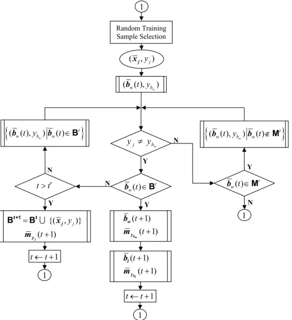
Figure 3.4 : Optimal separating hyperplane in SVM for a linearly nonseparable case. 36 Figure 4.1 : Flow graph of the BFDA algorithm. ... 43

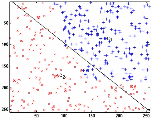
Figure 4.2 : Binary classification problem: class centers and selected initial border features depicted as circles, and the initial border line between classes when the decision is made based on only class centers... 46

Figure 4.3 : Partitioning of the two-dimensional feature space by using initial border feature vectors obtained at the end of the border feature selection procedure. ... 47

Figure 4.4 : Flow graph of the adaptation stage of the BFDA. ... 49

Figure 4.5 : Partitioning of the two-dimensional feature space by using the final border feature vectors obtained at the end of the adaptation procedure 50 Figure 4.6 : Block scheme of consensus strategy with k fold cross validation ... 51

Figure 5.1 : Reference feature space with randomly selected training samples .... 56

Figure 5.2 : The BFDA result ... 57

Figure 5.3 : The consensual-BFDA result... 57

Figure 5.4 : Linear SVM Result [C=2] ... 58

Figure 5.5 : RBF-SVM result [C=2, γ=32] ... 58

Figure 5.6 : AVIRIS data for the bands 50, 27 and 17... 59

Figure 5.7 : The ground truth of the AVIRIS data for 17 classes ... 65

Figure 5.8 : The thematic map of the BFDA result for data set 1... 65

Figure 5.9 : The thematic map obtained with the consensual BFDA and data set 2 66 Figure 5.10 : The thematic map obtained with the BFDA and data set 3 ... 66

Figure 5.11 : The thematic map obtained with the consensual BFDA and data set 4 67 Figure 5.12 : The thematic map obtained with the BFDA for data set 5. ... 68

Figure 5.13 : The thematic map obtained with the consensual BFDA for data set 6. 68 Figure 5.14 : Color composite image of Karacabey data for bands 4, 3 and 2 ... 71

Figure 5.15 : The ground truth of the Karacabey data with 9 classes ... 71

SINIR ÖZNİTELİKLERİNİN BELİRLENMESİ VE ADAPTASYONU: UZAKTAN ALGILAMA GÖRÜNTÜLERİNİN SINIFLANDIRILMASI İÇİN

YENİ BİR ALGORİTMA

ÖZET

Çeşitli sensörler dünya yüzeyinden çok miktarda data toplarlar. Toplanan bu dataların karakteristlikleri, kullanılan sensörün sahip olduğu görüntüleme geometrisine bağlıdır. Normalde, görüntü işleme tekniklerinin direk olarak uzaktan algılamaya uygulanması, sadece multispektral datalar için geçerli olabilir ki; bu datalar da göreceli olarak daha düşük sayıda öznitelik vektörüne sahiplerdir. Bu nedenle, 100-200 civarinda öznitelik vektörlerine (spektral band) sahip hiperspektral dataların analizi için gelişmiş algoritmalara ihtiyaç vardır.

Denetimli öğrenmede, eğitim işlemi çok önemlidir ve sınıflayıcının genelleme kabiliyetini belirler. Bu yüzden, yeterli sayıda eğitim örneği, düzgün bir sınıflama yapmak için istenir. Uzaktan algılamada, eğitim örneklerinin toplanması zor ve masraflı bir işlemdir. Bu yüzden, uygulamada sıklıkla karşılaşılan sınırlı sayıda eğitim örneğinin olmasıdır.

Geleneksel istatistiksel sınıflayıcılar, datanın belirli bir dağılıma sahip olduğunu kabul ederler. Gerçek veriler için bu tür bir yaklaşım geçerli olmayabilir. Ek olarak, hiperspektral datalarda doğru parametre tahmini oldukça zordur. Normalde sınıflandırma işleminde kullanılan band sayısı arttığı zaman, sınıfların ayrıntılı ve doğru olarak belirlenmesi beklenir. Yüksek boyutlu öznitelik uzayı için, yeni bir öznitelik dataya eklendiği zaman, sınıflandırma hatası azalır, fakat bunun yanı sıra sınıflandırma hatasının yanlılığı artar. Eğer sınıflandırma hatasının yanlılığındaki artış, sınıflandırma hatasındaki azalmadan daha büyük olur ise eklenen yeni özniteliğin kullanımı karar kuralının performansını düşürür. Bu etki Hughes etkisi olarak adlandırılır ve hiperspektral datada multispektral datadan daha zararlı olabilir.

Bu tezde bizim amacımız, istatistiksel dağılıma bağlı olmayan, sadece eldeki eğitim elemanlarını dayanan bir algoritma geliştirerek yukarıda özetlenen genel sınıflandırma problemlerinin üstesinden gelmektir. Bizim önerdiğimiz sınır özniteliklerinin belirlenmesi ve adaptasyonu (SÖBA) algoritması, karar yüzeylerine yakın sınır öznitelik vektörlerini kullanır ve bu sınır öznitelik vektörleri, maksimum marjin prensibini sağlayacak şekilde adapte edilerek, öznitelik uzayında doğru bölütlemenin yapılmasını sağlar.

Uzaktan algılama görüntülerinin sınıflandırılması için çok uygun olan SÖBA algoritması sınır özniteliği vektörlerinin eğitim kümesi elemanlarından seçilmesi ve eğitim kümesi elemanları yardımıyla adapte edilmesine dayanan yeni bir yaklaşımla geliştirilmiştir. Bu yaklaşım, özellikle enformasyon kaynağının sınırlı sayıda örnekle temsil edilmesi durumuyla karşılaşıldığında ve dağılımın gauss olmaması durumunda belirli öncül kabuller kullanmadığı için geleneksel istatistiksel sınıflayıcılara göre daha iyi sonuçlar üretir. Sınıflayıcılar, sınıf karar sınırlarına yakın olan eğitim örnekleri için hatalı karar vermeye eğilimlidirler. Bu yüzden, önemli öznitelik vektörleri sınıflandırma hatasını azaltmak için kullanılır. Önerilen sınıflandırma algoritması, hataya sebep olan eğitim örneklerini özel bir şekilde araştırarak, sınır öznitelik vektörlerini üretmek için adapte eder ve etiketli öznitelik vektörleri olarak sınıflandırmada kullanır.

SÖBA algoritması iki bölüme ayrılabilir. İlk kısım, sınıf merkezleri ve hatalı karar verilen eğitim örnekleri kullanılarak sınır öznitelik vektörlerinin başlangıç değerlerinin belirlenmesinden ibarettir. Bu yaklaşımla yönetilebilir sayıda sınır öznitelik vektörleri elde edilir. Algoritmanın ikinci bölümünde sınır öznitelik vektörlerinin adaptasyonu, learning vector quantization (LVQ) algoritmasıyla benzerlikler gösteren bir teknik kullanılarak gerçekleştirilir.Bu adaptasyon işleminde sınır öznitelik vektörleri, sınıf merkezleriyle olan mesafelerini uygun olarak sağlamak, farklı sınıflara ait komşu sınır öznitelik vektörleri arasındaki mesafeyi arttırmak için adaptif olarak güncellenir. Adaptasyon işlemi esnasında, sınıf merkezleri de aynı zamanda güncellenir. Sonraki sınıflandırma işlemi etiketli sınır öznitelik vektörlerine ve sınıf merkezlerine dayanır. Bu yaklaşımla herbir sınıf için uygun sayıda öznitelik vektörü algoritma tarafından atanır.

Denetimli öğrenmede eğitim süreci daha iyi sonuçlara ulaşabilmek için yansız olmalıdır. SÖBA algoritmasında başarım sınır öznitelik vektörlerinin başlangıç değerlerinin atanmasına ve eğitim örneklerinin eğitimde kullanılma sırasına bağlıdır. Bu bağımlılık sınıflayıcıyı nisbeten yanlı karar verici haline getirir. Konsensüs stratejisi ve çapraz sağlama birlikte kullanılarak, bu bağımlılıklar azaltılabilir.

Bu tezde, başlıca performans analizi ve karşılaştırmalar, AVIRIS datası kullanılarak yapılmışır. AVIRIS datası hiperspektral datadır ve sıklıkla litaratürde sınıflayıcıların performansını göstermek amacıyla kullanılır. Elde edilen ortalama eğitim, test başarımı ve kappa istatistiği Tablo.1 ’de gösterilmiştir. AVIRIS data kümesi 17 sınıf içerir. Data kümeleri 1 ve 2 için elde edilen sonuçlar 9 ve 190 bandlı durumlar için, SÖBA’ nın multispektral ve hipersipektral datadaki başarımını karşılaştırmak amacıyla verilmiştir. SÖBA’ nın başarımı, maximum likelihood, Fisher linear likelihood, correlation, matched filtering gibi çeşitli istatistiksel sınıflayıcı teknikleri ve destek vektör makinalarını (SVMs) içerecek şekilde verilmiştir. SÖBA’ nın diğer sınıflandırma teknikleriyle olan karşılaştırmasında sadece spektral öznitelikler dikkate alınmıştır.

Tablo 1: Ortalama Eğitim, Test Başarımları ve Kappa İstatistiği

EĞITIM TEST

DATA METOD _BAŞARIM

% Κ B

AŞARIM

% Κ

MAXIMUM LIKELIHOOD 84.83 0.82 67.56 0.63

FISHER LINEAR LIKELIHOOD _{63.7 0.59 47.3 0.42}

CORRELATION 48.4 0.43 37.2 0.31 MATCHED FILTER 32.8 0.24 36.1 0.29 KNN [K=5] 89.01 0.87 68.06 0.63 LINEAR SVM[C=40] 82.40 0.81 69.01 0.64 RBFSVM[γ=1,C=20] 86.10 0.83 71.73 0.67 SÖBA 94.05 0.89 70.82 0.66 1 KONSENSÜS SÖBA 96.41 0.95 73.36 0.69 KNN[K=5] 90.71 0.89 70.01 0.65 LINEAR SVM [C=10] 83.84 0.81 74.00 0.73 RBFSVM[γ=0.1,C=10] 87.74 0.86 77.64 0.74 SÖBA 99.46 0.99 76.40 0.73 2 KONSENSÜS SÖBA 100 1 78.71 0.75 SÖBA algoritmasıyla hem multispektral hemde hiperspektral datalar için tatminkar sonuçlar elde ettik. SÖBA, Hughes etkisi karşısında gürbüz bir algoritmadır. Bundan dolayı hem multispektral hem de hiperspektral datalar için uygundur. Ek olarak azınlık sınıf üyeleri, SÖBA algoritması tarafından geleneksel sınıflayıcıları gözönüne aldığımızda daha iyi bir şekilde korunur.

BORDER FEATURE DETECTION AND ADAPTATION: A NEW ALGORITHM FOR CLASSIFICATION OF REMOTE SENSING IMAGES

SUMMARY

Various types of sensors gather very large amounts of data from the earth surface. The characteristics of the data are related to sensor type which has its own imaging geometry. Therefore, sensor types affect processing techniques used in remote sensing. Normally, image processing techniques used directly in remote sensing are usually valid for multispectral data which is relatively in a low dimensional feature space. Therefore, advanced algorithms are needed for hyperspectral data which has at least 100-200 features (attributes/bands).

In supervised learning, the training process is very important and affects the generalization capability of a classifier. Therefore, enough number of training samples is required to make proper classification. In remote sensing, collecting training samples is difficult and costly. Consequently, a limited number of training samples is often available in practice.

Conventional statistical classifiers assume that the data has a specific distribution. For real world data, these kinds of assumption may not be valid. Additionally, proper parameter estimation is difficult, especially for hyperspectral data. Normally, when the number of bands used in the classification process increases, precise detailed class determination is expected. For high dimensional feature space, when a new feature is added to the data, classification error decreases, but at the same time, the bias of the classification error increases. If the increment of the bias of the classification error is more than the reduction in classification error, then the use of the additional feature decreases the performance of the decision rule. This phenomenon is called the Hughes effect, and it may be much more harmful with hyperspectral data than with multispectral data.

Our motivation in this thesis is to overcome some of these general classification problems by developing a classification algorithm which is directly based on the available training data rather than on the underlying statistical data distribution. Our proposed algorithm, border feature detection and adaptation (BFDA), uses border feature vectors near the decision boundaries which are adapted to make a precise partitioning in the feature space by using maximum margin principle.

The BFDA algorithm well suited for classification of remote sensing images is developed with a new approach to choosing and adapting border feature vectors with the training data. This approach is especially effective when the information source has a limited amount of data samples, and the distribution of the data is not necessarily Gaussian. Training samples closer to class borders are more prone to generate misclassification, and therefore are significant feature vectors to be used to reduce classification errors. The proposed classification algorithm searches for such error-causing training samples in a special way, and adapts them to generate border feature vectors to be used as labeled feature vectors for classification.

The BFDA algorithm can be considered in two parts. The first part of the algorithm consists of defining initial border feature vectors using class centers and misclassified training vectors. With this approach, a manageable number of border feature vectors are achieved. The second part of the algorithm is adaptation of border feature vectors by using a technique which has some similarity with the learning vector quantization (LVQ) algorithm. In this adaptation process, the border feature vectors are adaptively modified to support proper distances between them and the class centers, and to increase the margins between neighboring border features with different class labels. The class centers are also adapted during this process. Subsequent classification is based on labeled border feature vectors and class centers. With this approach, a proper number of feature vectors for each class is generated by the algorithm.

In supervised learning, the training process should be unbiased to reach more accurate results in testing. In the BFDA, accuracy is related to the initialization of the border feature vectors and the input ordering of the training samples. These dependencies make the classifier a biased decision maker. Consensus strategy can be applied with cross validation to reduce these dependencies.

In this thesis, major performance analysis and comparisons were made by using the AVIRIS data. The AVIRIS data is a hyperspectral data set and is often used in the literature to demonstrate performancec of classifiers. Average training, testing accuracies and kappa statistics are given in Table.1. The AVIRIS data set contains 17 classes. The results were obtained for data sets 1 and 2 for 9 and 190 features respectively to make proper comparison of the BFDA with multispectral and hyperspectral data. The performance of the BFDA was compared with other classification algorithms including support vector machines and several statistical classification techniques such as maximum likelihood, Fisher linear likelihood, correlation and matched filtering algorithms. Only spectral features were taken into account in the comparison of BFDA with other classification techniques.

Table 1: Average Training ,Testing Accuracies and Kappa Statistics TRAINING TESTING DATA SET METHOD ACCURACY % Κ A CCURACY % Κ MAXIMUM LIKELIHOOD 84.83 0.82 67.56 0.63

FISHER LINEAR LIKELIHOOD 63.7 0.59 47.3 0.42

CORRELATION 48.4 0.43 37.2 0.31 MATCHED FILTER 32.8 0.24 36.1 0.29 KNN[K=5] 89.01 0.87 68.06 0.63 LINEAR SVM[C=40] 82.40 0.81 69.01 0.64 RBFSVM[γ=1,C=20] 86.10 0.83 71.73 0.67 BFDA 94.05 0.89 70.82 0.66 1 CONSENSUAL BFDA 96.41 0.95 73.36 0.69 KNN[K=5] 90.71 0.89 70.01 0.65 LINEAR SVM [C=10] 83.84 0.81 74.00 0.73 RBFSVM[γ=0.1,C=10] 87.74 0.86 77.64 0.74 BFDA 99.46 0.99 76.40 0.73 2 CONSENSUAL BFDA 100 1 78.71 0.75

Using the BFDA, we obtained satisfactory results with both multispectral and hyperspectal data sets. The BFDA is a robust algorithm with the Hughes effect. Therefore it is well-suited for both multispectral and hyperspectral data. Additionally, rare class members are more accurately classified by the BFDA as compared to conventional statistical methods.

1. INTRODUCTION

Electromagnetic radiation from visible to microwave regions reflected from the earth’s surface can be measured by passive and active sensors. These measurements can be taken in to account as spectral feature vectors (attributes) for classification problems. Both the sensor types employed for gathering information, and the size of feature vectors (total number of bands) designate the design considerations of classification algorithms for multispectral and hyperspectral remote sensing.

1.1 Multispectral and Hyperspectral Data Structure

The multispectral sensors collect data in a small number of bands (features) from the different regions of the electromagnetic spectrum. Remote sensing images acquired by multispectral sensors, such as the widely used Landsat Thematic Mapper (TM) sensor, have shown their usefulness in numerous earth observation (EO) operations. In general, relatively small number of acquisition channels that characterizes multispectral sensors may be sufficient to discriminate among different land-cover classes (e.g., forestry, water, crops, urban areas, etc). However, their discrimination capability is very limited when different types (or conditions) of the same species (e.g., different types of forest) are to be recognized. For a specific band in multispectral data, measured value is averaged through the band with typically 100-200 nm in width. Therefore, narrow spectral features masked by stronger proximal features may not be readily discriminated across the spectral sampling range [1]. As an example, 17 spectral signatures for 17 classes have been depicted in Figure 1.1. As we can see from the Figure 1.1, discriminating these 17 classes from each other is a very complex classification problem and only using multispectral sensors can not be sufficient to support precise discrimination, for especially detailed class identification for the same species. Therefore, making individual measurements in a narrow band to detect instantaneous variations of specific target response is required.

Figure 1.1: Spectral Signature of 17 Classes

Hyperspectral sensors can be used to deal with this problem. Hyperspectral sensors collect data using hundreds of narrow (2-20 nm in width) contiguous wavelength intervals over visible, near infrared (VNIR), short wave infrared (SWIR) and the thermal infrared (TIR) wavelength regions. Hyperspectral imaging spectrometers were subsequently able to retrieve reflectance spectra such that the data associated with each pixel approximated the true spectral signature of a target material, with sufficiently high signal-to-noise ratio (SNR) across the full contiguous wavelength range (normally 400-2500 nm). This collected data is represented as a hyperspectral image cube as depicted in Figure 1.2 [2]. In this cube, x and y axes specify the size of the images (spatial coordinates), whereas the z axis denotes the number of bands (features) in the hyperspectral data. The detailed spectral response of a pixel assists in providing accurate and precise extraction of information than is obtained from multispectral imaging. It is also possible to address various additional applications requiring very high discrimination capabilities in the spectral domain. From a methodological viewpoint, the automatic analysis of hyperspectral data is not a trivial task. In particular, it is made complex by many factors, such as the large

spatial variability of the hyperspectral signature of each land cover class, atmospheric effects and the curse of dimensionality.

Figure 1.2: The Hyperspectral Cube

The processing of hyperspectral data remains a challenge since it is quite different from multispectral processing. Cost effective and computationally efficient procedures are required to process hundreds of bands (spectral resolution) consisting of 10-bit to 16-bit data (radiometric resolution).

The data gathered by The Airborne Visible/Infrared Imaging Spectrometer (AVIRIS) was used in the experiments in this thesis. This sensor was the first to acquire image data in continuous narrow bands simultaneously in the visible to shortwave infrared (SWIR) wavelength regions. The original AVIRIS data has 224 bands and spectral range of the data is 400-2450 (nm). For a 12-bit reflectance data, the number of discrete points in the 220-dimentional space is (212)220. One enormous advantage of hyperspectral imaging is the concept of “Spectral Signature”. A spectral signature refers to the one-dimensional plot of brightness values of a pixel in the spectral domain, which is related to the characteristics of the observed material on the Earth surface, at a specific location. Each individual material has its own spectral signature. Data analysis is aimed at extracting meaningful information from remotely sensed data. A limited number of image analysis algorithms have been developed to exploit the extensive information contained in hyperspectral imagery in many applications such as military target detection, mineral mapping, pixel and sub-pixel level land cover classification, etc. Most of these algorithms have originated from the ones used

x y

for analysis of multispectral data, and thus have limitations. A novel classification algorithm called border feature detection and adaptation (BFDA) is proposed in this thesis for both multispectral and hyperspectral data classification to help reduce some of these problems.

1.2 General Classification Problem

Two main classification types can be considered. They are supervised and unsupervised methods. In this thesis, a supervised classification algorithm was introduced for both multispectral and hyperspectral images. For supervised learning, we have two different sets, one for training and the other one for testing. Sets of training and testing samples have features with their belongings labels. Ground truth refers to the reference set used for selecting samples to generate training and testing sets.

The classification problem occurs in its simplest form as the two class problem (binary case classification problem). It involves two partially disjoint finite sets X and Y, and an object z∉ XUY is to be classified as a member of X or Y. The multi-class problem occurs when there are additional sets corresponding to other multi-classes. The main goal of the classification problem is to find a classifier that can predict the label of new unseen data samples correctly. This can be achieved by learning from the given labeled data (training set). The test set correctness of classification is the main criterion used to evaluate a given classifier.

1.3 Problem Description and Aims of This Thesis

In supervised learning, a selected set of labeled training data is used during learning. The performance of a classification algorithm is closely related to how the labeled training data set is correlated with the unlabeled testing data set. Errors are more difficult to control in the case of detection of rare class members. Especially in hyperspectral data classification, there is a large number of spectral bands, and a relatively low number of labeled training samples [3]. Therefore, one of the main difficulties is related to the small ratio between the number of available training samples and the number of features. This may cause unsatisfactory estimates of the

class-conditional probability density functions used in standard statistical classifiers. As a consequence, when the number of features given as input to the classifier over a given number of training samples is increased, the classification accuracy decreases. This behavior is known as the Hughes phenomenon [3]. Our motivation in this study is to overcome some of these general classification problems, by developing a classification algorithm which is directly based on the available training data rather than on the underlying statistical data distribution.

In the literature, four main approaches can be identified to make statistical classification methods applicable for hyperspectral data classification problem. These approaches are:

1) Regularization of sample covariance matrix by using sample and common covariance matrices together [4,5].

2) Adaptive statistical estimation by the exploitation of the classified (semi- labeled) samples (e.g., Expectation maximization algorithm, EM) [6,7]. 3) Preprocessing techniques based on feature selection/extraction, aimed at

reducing/transforming the original feature space into another space of a lower dimensionality (e.g., Fisher Linear Discriminate (FLD), Discriminate Analysis Feature Extraction (DAFE), Decision Boundary Feature Extraction (DBFE), Projection Pursued (PP), etc.) [8-10].

4) Analysis of the spectral signature to model the classes [11,12].

Many supervised classification techniques have been used for multispectral and hyperspectral data classification, such as the maximum-likelihood classification, neural networks and support vector machines. Practical implementational issues and computational load are additional factors to evaluate classification algorithms. Statistical classification algorithms are fast and reliable, but they assume that the data has a specific distribution. For real world data, these kinds of assumptions may not be sufficiently accurate, especially for low probability classes. The k-nearest neighborhood algorithm is another simple and effective classification method.

In recent years, kernel methods such as support vector machines (SVMs) have demonstrated good performance in hyperspectral data classification [13]. Some of

the drawbacks of SVMs are the necessity of choosing an appropriate kernel function and time-intensive optimization. In addition, the assumptions made in the presence of samples which are not linearly separable are not necessarily optimal. Parallel, self-organizing hierarchical neural networks (PSHNNs) also achieve high classification accuracy [14]. By using parallel stages of neural network modules, hard vectors are rejected to be processed in the succeeding stage modules, and this rejection scheme is effective in enhancing classification accuracy. Consensual classifiers are related to PSHNNs, and also reach high classification accuracies [15,16].

Combining different classification algorithms to get high classification accuracy is a reliable approach [17]. It is also possible to combine the outputs of classifiers which use the same classification algorithm but are differently structured to make the decisions of the individual classifiers sufficiently independent from each other [18]. For example, this can be done by changing the input order of training samples. In this thesis, a new classification algorithm well suited for classification of remote sensing images is developed with a new approach to choosing and adapting border feature vectors with the training data. This approach is especially effective when the information source has a limited amount of data samples, and the distribution of the data is not necessarily Gaussian. Training samples closer to class borders are more prone to generate misclassification, and therefore are significant feature vectors to reduce classification errors. The proposed classification algorithm searches for such error-causing training samples in a special way, and adapts them to generate border feature vectors to be used as labeled feature vectors for classification.

The BFDA algorithm can be considered in two parts. The first part of the algorithm consists of defining initial border feature vectors using class centers and misclassified training vectors. With this approach, a manageable number of border feature vectors are achieved. The second part of the algorithm is adaptation of border feature vectors by using a technique similar to the learning vector quantization (LVQ) algorithm [19]. In this adaptation process, the border feature vectors are adaptively modified to support proper distances between them and the class centers, and to increase the margins between neighboring border features with different class labels. The class centers are also adapted during this process. Subsequent classification is based on labeled border feature vectors and class centers. With this

approach, a proper number of feature vectors for each class is generated by the algorithm.

1.4 Organization of the Thesis

This thesis is organized in six chapters. Feature extraction or dimensionality reduction is needed for classification of hyperspectral data when classification algorithms based on statistics such as maximum likelihood is used. In chapter 2, a brief discussion is given about feature extraction, and the method called projection pursued (PP) [9] is mentioned. Using spatial features in addition to spectral features improves classification accuracy. A spatial feature extraction method [20] is also discussed in chapter 2. We categorized classification techniques in three parts and explained some important ones in chapter 3 to make precise comparison with our proposed algorithm, the BFDA [21]. These categories are parametric, non-parametric and kernel methods. Methods based on statistics such as maximum likelihood (ML) and expectation maximization (EM) [7] are parametric methods, whereas k-nearest neighbor (KNN), grow and learn (GAL) [22], and self-organizing map (SOM) [19] are non-parametric methods. In addition, kernel methods such as support vector machines (SVMs) [13,23] are also explained in chapter 3 as a relatively new generation of techniques for classification and regression problem. Our proposed algorithm border feature detection and adaptation (BFDA) [21] is introduced in chapter 4. Additionally, to reach better classification accuracies, usage of the BFDA as an individual classifier in a consensual scheme and a safe rejection scheme for the BFDA are also provided. Descriptions of the data set and experiments designed are introduced, and detailed comparison of methods is discussed in chapter 5. Conclusions and future work are given in chapter 6.

2. FEATURE EXTRACTION

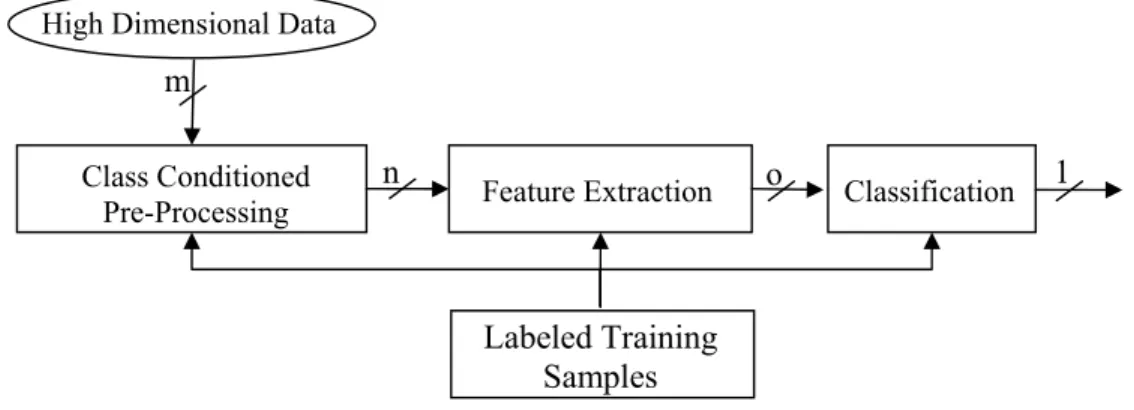
In this section, feature dimension reduction for increasing class discrimination, and spatial feature extraction from conventional spectral features are discussed. In general, basic remote sensing classification systems include a module of feature extraction. This module is necessary in hyperspectral data classification for dimension reduction especially when parametric classifier based on density estimation is used. The basic classification flow graph for remote sensing including feature extraction is depicted in Figure 2.1.

Figure 2.1: TheBasic Classification Flow Graph

The aim of feature extraction is to reduce dimensionality to support proper density estimation and to increase class separability at the same time. To make a proper comparison between parametric classifiers and our proposed algorithm, the BFDA, concept of feature extraction for dimensionality reduction for increasing class discrimination is discussed, and some important methods used in the experiments are introduced in this chapter. We first explain feature extraction for dimensionality reduction. Then, we discuss how spatial features are extracted from spectral ones. The effects on classification accuracy are shown with experiments. In addition, it is also possible to apply dimensionality reduction after extraction of spatial features.

Remotely

Sensed Data m _ExtractionFeature n Classifier 1 Result

Labeled Training Samples

2.1 Methods for Feature Dimension Reduction

High-Dimensional space characteristics are a major issue in design considerations of classifiers for hyperspectral data classification. Therefore, it is useful to understand high dimensional feature space characteristics. It has been proven that as the number of dimensions increases, volume of a hypercube (whole feature space) concentrates in the corners, and the volume of a hyperellipsoid concentrates in an outside shell in the feature space [24]. These characteristics have two important consequences for high dimensional data: 1) High-dimensional data is mostly empty, which implies that multivariate data is in a low dimensional structure. 2) Normally distributed data will have a tendency to concentrate in the tails, while uniformly distributed data will be more likely to be collected in the corners. Together, these consequences make density estimation more difficult in the high-dimensional feature space. Under these circumstances, it would be difficult to obtain accurate results with most density estimation procedures.

The required number of labeled samples for supervised classification increases as a function of dimensionality. The required number of training samples is linearly related to the dimensionality for a linear classifier and to the square of the dimensionality for a quadratic classifier. It has been estimated that as the number of dimensions increases, the sample size needs to increase exponentially in order to obtain an effective estimate of multivariate densities [25,26].

The second-order statistics is often important in the process of discriminating among classes. In hyperspectral data, neighbor bands are usually highly correlated. Therefore, most of the data is distributed a long a few major components producing a hyperelipsoid-shaped data distribution characterized by second order statistics [27]. It is to be expected that high-dimensional data contains more information. At the same time, the above characteristics tell us that it is difficult to extract such information with techniques which are based on density estimation since these are usually based on computations at full dimensionality requiring a substantial number of labeled data. Hughes proved that with a limited number of training samples, there is a penalty in classification accuracy as the number of features increases beyond some point [3].

From classification viewpoint, especially for classification algorithms based on statistics, lower dimensional feature vectors are needed in order to make proper density estimation. Some widely used feature extraction methods for dimensionality reduction are principle component analysis (PCA), discriminate analysis feature extraction (DAFE), decision boundary feature extraction (DBFA), and projection pursuit (PP). It is also very useful to mention the difference between dimensionality reduction for data compression and classification. For data compression, most important aim is to keep most informative components but for data classification most important aim is to keep most discriminative components.

Principle component analysis assumes that the distribution takes the form of a single hyperellipsoid, such that its shape and dimensionality can be determined by mean-vector and covariance matrix of the distribution. A problem with this method is that it treats the data as if it is a single distribution. Principle components analysis is more appropriate for data compression than for class discrimination [25].

DAFE is a method that reduces the dimensionality, optimizing the Fisher ratio [28]. If the total number of classes is c than the final dimension will be c-1 after DAFE. It performs the computations at full dimensionality, requiring a large number of labeled samples in order to accurately estimate parameters.

DBFE is an algorithm based directly on decision boundaries [8]. This method also predicts the number of features necessary to achieve the same classification accuracy as in the original space. DBFE has the advantage of finding the necessary feature vectors. One disadvantage of this method is that it demands a high number of training samples in a high-dimensional space. This occurs because it computes the class statistical parameters at full dimensionality.

When there are only a limited number of training samples, method of projection pursuit (PP) can be used [9,29,30]. This method performs the computation in a lower dimensional subspace that is a result of a linear projection from the original high dimensional space. This dimension reduction increases the ratio of labeled samples per feature, resulting in better parameter estimation and better classification accuracy.

2.1.1 Dimension Reduction via Projection Pursuit (PP)

Feature extraction for dimensionality reduction is needed for parametric classifiers, especially in high-dimensional feature space. Parametric classifiers use first and second order statistics whose parameters are estimated by using only labeled training samples. From the nature of the classification problem for hyperspectral data, these labeled training samples are not sufficient to make proper estimation of these parameters. Therefore dimensionality reduction is needed in hyperspectral data classification especially for parametric classifiers.

The basic dimensionality reduction scheme is depicted in Figure 2.2.

Figure 2.2: Dimensionality Reduction by Projection Pursuit

X is a multivariate data set and it is dxN dimensional matrix, Y is the resulting dimensionality reduced projected data which is mxN dimensional matrix and A is the transform matrix which is a dxm dimensional matrix. Dimension reduction also desired to include improvement of discrimination of classes. Therefore the algorithm should optimize the projection index I(AT_{X) to increase class discrimination. In}

general, the projection index is related to first and second order statistics such as mean and covariance matrix of the training samples as in Bhattacharyya distance index which is widely used for discrimination measurement. The PP uses Bhattacharyya distance between two classes as the projection index because of its relationship with Bayes-classification accuracy, and its use of both first order and second order statistics [31].

1 2 1 1 2 2 1 2 1 1 2 1 1 2 ( ) ( ) (M -M )+ ln 8 2 2 Y Y T Y Y Y Y Y Y Y Y −  ∑ + ∑  ∑ + ∑   _{ } = − _{ }     ∑ ∑     T I A X M M (2.1) X Dimensionality Reduction [AT] Y= ATX

where M_jYand ∑_jYare the mean vector and covariance matrix, respectively, of the jth class in the projected subspace Y. In the case of more than two classes, the minimum Bhattacharyya distance among the classes can be used after the Bhattacharyya distances are calculated for all combinations of two classes. Then, the minimum of the Bhattacharyya distance is chosen as

1 2 1 1 2 2 1 2 1 1 2 2 1 1 ( ) min ( ) (M -M )+ ln 8 2 2 i i Y Y i i i i T Y Y i i Y Y Y Y _{i i} Y Y i C − ∈   _{∑ + ∑}   _{∑ + ∑ }    _{ } = _ − _{   }   ∑ ∑  _{ }    _{ }   T I A X M M (2.2)

C is the number of combinations of pair of two classes. Assuming that total number of classes is L, C is given by ! 2!( 2)! L C L = − (2.3)

The main advantage of PP is that of calculating the projection index in a low dimensional space. In addition, nearest spectral responses are correlated with each other for hyperspectral data. Therefore band grouping is applied for dimensionality reduction as a preprocessing in the PP. First and second order statistics are calculated in this low dimensional space much more accurately.

Thus, the global projection index to be maximized is the minimum Bhattacharyya distance among the classes. A sequential aspect of this algorithm is that it projects groups of neighboring bands while maximizing the minimum Bhattacharyya distance in the projected subspace. Maximization can be done with a known numerical optimization algorithm.

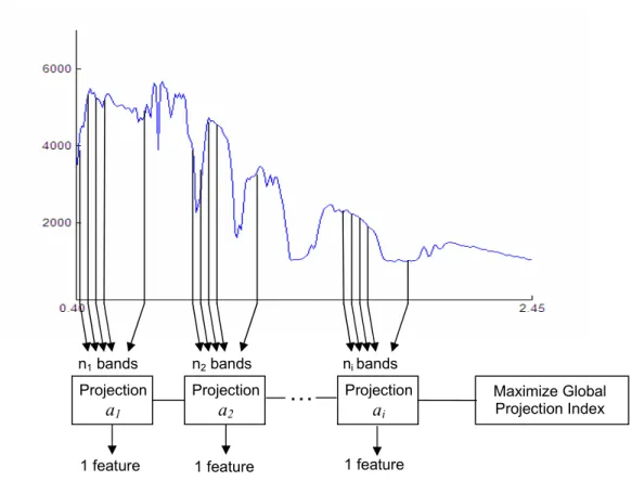
As explained above, projection indices for optimizing discrimination are parametric, and estimation of these parameters is carried out in a lower dimensional space. The computations at a lower-dimensional space enable PP to better handle the problem of small numbers of samples. In Figure 2.3, band grouping in projection pursuit is depicted. An iterative procedure to estimate ai’s is described in the following steps

Figure 2.3: Band Grouping in Projection Pursuit 1) Make an initial guess for every ai for each group of adjacent bands.

2) Maintaining the rest of ai’s constant, compute the a1 (the vector that projects the

first group of adjacent bands) that maximizes the minimum Bhattacharyya distance. 3) Repeat the procedure for each of the groups while ai’s, for i≠ j, remain constant.

4) Once the last group of adjacent bands is projected, repeat the process starting from step 2 (compute all aj’s sequentially) until convergence.

In Figure 2.4 projection pursuit is used as a preprocessing technique for dimensionality reduction by optimizing a projection index. After the processing described above has been applied, a scheme of feature extraction such as discriminate analysis feature extraction (DAFE) or decision boundary feature extraction (DBFA) can be used in the lower dimensional feature space. As a

Projection a1 Maximize Global Projection Index Projection a2 n1 bands n2bands Projection ai ni bands

1 feature 1 feature 1 feature

consequence, the most discriminative features and lower dimensional space (m<n<o) can be achieved.

Figure 2.4: PP Based Preprocessing Technique Used for Dimensionality Reduction It is obvious that there are a variety of projection indices which can be used in the PP algorithm. Such a projection index related to correlation between features is as follows. Highly correlated features are combined with each other to form a group. The adjacent features of the data exhibit high correlation. Therefore, the hyperspectral subspace is partitioned into subspaces based on correlation existing between adjacent features. The correlation ρ for bands i and j is given by

ij ij

ii jj

ρ = ∑

∑ ∑ (2.4)

where ∑_ijis the element of the covariance matrix for band i versus band j and ∑ii

and ∑_jjare the variances of the ith _{and j}th _{features of the data [31]. The parameter} ij

ρ indicates the covariance between bands i and j. The variables i and j vary from 1 to d, where d is the dimensionality of the subspace. The correlation measure C of the hyperspectral subspace quantifies the correlation between two bands, i.e. C gives the minimum of all the correlations between every pair of bands in the subspace. Therefore, ( ) n ij n C =min ρ (2.5) Class Conditioned Pre-Processing High Dimensional Data

Feature Extraction Classification

Labeled Training Samples

n o 1

where C_n represents correlation of the nth subspace .

Supervised and automatic selection procedures can be applied for feature subset selection procedure. It is also possible to select feature size fixed or adaptively chosen.

2.2 Spatial Feature Extraction

Spatial variations of the spectral features in a predefined sub-image with appropriate sub-image size can be used as effective features in remote sensing applications [32,33]. Features based on spatial variations are called texture features as well. Texture features are robust features on noisy remote sensing data such as the data acquired by synthetic aperture radar (SAR). Especially for SAR data classification, noise is an important concern to deal with in order to achieve sufficient classification accuracy. The noise called speckle has its origin in collecting data by using active sensors in microwave frequencies. Therefore, using spatial variations instead of spectral response from individual pixels is necessary to make proper SAR classification. Gray level co-occurrence matrix statistical parameters can be used as texture features [33].

There are three different texture categories. They are course texture (neighboring points similar), fine texture (neighboring points different) and directional texture (courser in one direction). Because of speckle noise in SAR data, fine texture properties are typical. For hyperspectral data, texture category is typically course texture. Therefore, we expect to find more homogeneous areas in hyperspectral data classification.

Spatial filtering can be used to generate more homogenous regions and thereby improve classification performance in hyperspectral data classification [20]. The spatial filter can be a simple mean filter, which uses standard deviation as a homogeneity criterion. Using a homogeneity criterion, sub-image size (window size) changes adaptively to achieve more homogeneous regions in the spatial domain. If homogeneity test passes, then the mean value of the pixels in the window is assigned to the center pixel of the sub-image.

Formally, given an image I(m,n), the median filter can be shown by

{

}

( , ) ( , )

median

I m n =median I m k n l , (k,l) A− − ∈ (2.6)

Where A is the neighborhood over which the median is applied. Median filters are most useful in mitigating the effects of salt and pepper noise that arises typically due to isolated pixels incorrectly switching to opposite intensity.

In this thesis, we extracted spatial features such as mean and variance for sub-image size (window size) from 3x3 to 9x9, and obtained combined classification results which are based on individual spatial and spectral features by using a consensual rule to reach better classification accuracy. In this way, we showed the use of spatial features together with spectral features on hyperspectral data classification.

3. TYPES OF CLASSIFIERS

The aim of classifiers is to partition the feature space into an exhaustive set of nonoverlapping regions to reach high classification accuracy by using some rules related to discrimination of the classes. These discrimination rules can be based on statistical theory or computational methods such as neural networks. Decision boundaries can be determined by a threshold function obtained by equalization of the neighbor class discrimination rules. In this chapter, a brief summary is given on classifiers used in the experiments to make a detailed comparison between the proposed classification algorithm, the BFDA, and other conventional classification methods used.

We can categorize classifiers into three types. They are parametric, non-parametric and kernel methods. For parametric methods, maximum likelihood (ML) and expectation maximization (EM) are described [35,36]; k-nearest neighbor (KNN) [37], grow and learn (GAL) [22] and self organizing map (SOM) [19] are discussed as examples of non-parametric methods. In recent years, use of support vector machines for classification and regression problems has been increasing rapidly. Support vector machines (SVMs) are discussed as an example of kernel methods [13]. SVM is initially a binary classifier. Therefore, proper hierarchical methods are needed to combine binary classifiers outputs to generate multi-class classification results.

An important performance criterion is overall classification accuracy for classifiers. Additionally, detection of rare class members is a desirable specification. Kappa statistics was used to measure reliability of decisions made [34]. In addition, practical implementation issues and computational load are important design concerns to make a proper comparison of the classifiers.

3.1 Statistical Classifiers

Classifiers based on statistics are widely used, especially in low dimensional feature spaces. In general, they are parametric classification methods, and their drawbacks are proper parameter estimation needs and pre-assumptions on their distributions made before classification. Especially in high dimensional feature space, difficulties of proper parameters estimation can be reduced by using dimension reduction methods for increasing class discrimination such as DAFE, DBFA and PP [35]. It is also difficult to detect rare class members with statistical methods. In this section, a brief summary is given on statistical methods such as maximum likelihood (ML) and expectation maximization (EM) [36].

3.1.1 Maximum Likelihood Classifier

Conditional probability density function (pdf) is used as discrimination rule in the maximum likelihood (ML) classifier. If the number of classes is m, then there are m discrimination functions that can be defined by using conditional probability density function as follows:

(

)

The label of the class which makes the discrimination rule maximum is assigned as the class of x:

{

}

In this approach, the classification problem is reduced to estimate some parameters which are related to probability density function (pdf). The Gaussian density function is widely used for classification problems because it has convenient properties and fits many processes in nature. The Central Limit Theorem states that if a random observation is made on a collection a large of number of independent random quantities, the observation will have a Gaussian distribution. If the random variable is one-dimensional, then the Gaussian density function is given by

(

)

In remote sensing data classification problems random variable is a vector. Especially for hyperspectral data classification, the dimension of the random variable may be larger than 100. The AVIRIS data set which is used in the experiments can be cited as an example of hyperspectral data. The original dimension (total number of bands/attributes) of the AVIRIS data set is 224. For multispectral data such as Landsat and Spot, the numbers of dimensions are 7 and 4, respectively. In this case, assuming N dimensions, the pdf can be written in the vector form as

(

)

where x_i is random variable, µ_i the mean vector of the ith class, and ∑_i is the covariance matrix of the ith class, respectively. The Gaussian pdf is also called normal distribution and is depicted by ( ,N µ_i ∑_i). The unbiased estimaties of the multidimensional Gaussian pdf parameters are calculated as follows: assuming a labeled training data set {( , ),( , ), ,( , )}x1 y1 x2 y2 ⋅ ⋅ ⋅ xn yn where the training

vectors are _∈ N,_i=1,...,_n

i

x , the class labels arey_i∈{1, 2, , }⋅ ⋅ ⋅ m , n is the total number of training samples, and m is the number of classes, class means are estimated as 1 ˆ _{,{ | , 1, , }} 1 i n_i x_j x_j y_j i i m n j_i µ = ∑ = = ⋅ ⋅ ⋅ = (3.6)

where n_i is the total number of training samples for class i. The covariance matrix estimate of the ith class is given by

1 ˆ _{ˆ)( ˆ ) ,{ | , 1, , }} 1 ₁ T i i i n_i ( y_j i i m n_{i j} µ µ ∑ = ∑ − − = = ⋅ ⋅ ⋅ − ₌ xj xj xj (3.7)

Logarithmic version of the pdf is widely used as a discrimination function as follows:

(

)

(

)

which is a quadratic function and is commonly used in the Gaussian maximum likelihood (GML) classifier [38].

The minimum expected error that can be achieved in performing classification is referred to as the Bayes’ error. A decision rule that assigns a sample to the class with highest a posteriori probability (the MAP classifier) achieves the Bayes’ error [31]. A posteriori probability can be written as follows by using Bayes’ rule:

(

) (

)

(

)

If the prior probabilities of classes are known, and they are used to multiply with the class density functions the resulting algorithms are called minimum error classifiers, because they result in the theoretically minimum overall error:

(

)

(

)

( ) , ( ), 1..

i

C i i i

g x = p x C = p x C p C i= m (3.10)

In practice, the prior class probabilities are often not known need to be estimated. Class conditional density functions (pdf’s) also need to be estimated from a set of training samples. For a high dimensional feature space, when a new feature is added to the data, the Bayes error decreases, but at the same time the bias of the classification error increases. The reason of this increase is that more parameters need to be estimated from the same number of training samples. If the increase in the

bias of the classification error is more than the decrease in the Bayes error, then the use of the additional feature decreases the performance of the decision rule. This phenomenon is called the Hughes effect [3]. The larger the number of the parameters that need to be estimated, the more severe the Hughes phenomenon can be. Therefore, when the dimensionality of data and the complexity of the decision rule increase, the Hughes effect can become more severe. It is obvious that, linear classifiers such as minimum distance to mean (minimum Euclidean distance) are less affected by the Hughes effect than the quadratic classifiers such as the Gaussian maximum likelihood (GML) classifier [36,38]. The discriminatant function for the minimum distance to mean classifier is given by

( ) )( ) , 1...

i

T

C i i

g x =(x−µ x−µ i= m. (3.11)

In addition, Fisher’s linear discriminant classifier assumes that each class has the same covariance matrix called the common covariance matrix which can be calculated by using all available labeled samples (training samples) [36]. The Fisher’s linear discriminant classifier is given by

1 ( ) ) ( ) , 1... i T C i i g x ₌(_x−µ _∑− _x−µ i₌ m_{. (3.12)}

3.1.2 Expectation Maximization (EM)

Performance of a classifier is usually related to the degree of discrimination function complexity. More complex classifiers need much more labeled training samples to make a proper estimation of parameters used in the discrimination function. Especially in remote sensing, labeled samples are limited. This drawback affects classification accuracy in a negative way especially when the feature vector size increases. Parametric classifiers such as quadratic ones are much more affected by limited training samples. In order to enhance estimation of parameters, unlabeled samples can be incorporated together with limited labeled ones. In the following discussion, enhancement of Gaussian density function parameters (prior probabilities, mean vectors and covariance matrices) is achieved via expectation maximization (EM) algorithm [38].

When individual classes are multivariate Gaussian, the ML estimates of the parameters of the mixture density consisting of the m normal classes are considered. We assume ith class ni labeled training samples are available. We will denote these

training samples by zik where i indicates the class (i=1,…,m), and k is the index of

each particular sample. In addition, we assume that N unlabeled samples denoted by xk are available to enhance the mixture density given by

1 ( ) m i i( ), 1... i p θ α p i m = =

∑

The EM equations for approximating the ML estimates of the parameters of the mixture density are the following [39]:

1 1 ( , ) ( ) t t t N i i k i i t k k t i p x p x N α µ θ α + = ∑ =

∑

∑

∑

∑

(

)(

)

(

)(

)

(

)

∑

∑

∑

∑ are the mean vector and the covariance matrix of class i at iteration t. The parameter set _θt _{contains all the prior probabilities, mean vectors and}

covariance matrices. The ML estimates are obtained by starting from an initial point in the parameter space and iterating through the above equations. Reasonable initial values are obtained by using the training samples alone. An important practical point

classification accuracy, this might not always be the case in practice. The reason for this is the deviation of the real world situations from the models that are assumed. Therefore, additional care must be taken when supervised-unsupervised learning is used in practice. Designing a classifier by using the training sample alone and then trying to improve classification accuracy by enhancing statistics via incorporating unlabeled samples with labeled ones is an efficient indicator to show the contribution of enhancement of statistics. If the performance of the classifier is not satisfactory, then a new set of unlabeled samples is selected and used to enhance the statistics to reach more accurate classification results.

3.2 Nonparametric Methods

Classification algorithms based on statistics assume that data has a specific distribution, typically a Gaussian distribution. For real world data, such assumptions may not be valid. Additionally, statistical classifiers are parametric classifiers, and proper estimation of parameters is needed. Especially with limited number of labeled training samples, which is very common situation in remote sensing, there are additional difficulties involved in proper parameter estimation of class distributions. These difficulties get harder in high dimensional feature space as compared to low dimensional feature space. Therefore, some complementary methods such as dimensionality reduction and enhancing estimation of parameters are needed for parametric methods to get satisfactory results. In addition, increasing classification accuracy is not guaranteed by using methods for enhancing estimation of parameters. Therefore, nonparametric methods are widely used to overcome these classification problems summarized above. Main aim of nonparametric methods is to extract maximum information from limited number of labeled samples to make an appropriate decision. Directly using training samples is an important specification of the nonparametric methods to describe feature space. Another advantage of nonparametric methods is stability of obtained classification accuracies with dimensionality changes. Therefore, the Hughes effect is less harmful for nonparametric methods than parametric ones. Training process often takes more time for nonparametric methods, and that could be a disadvantage. Our proposed algorithm the BFDA is also a nonparametric classifier. Therefore, in this section we explain some nonparametric methods such as the k-Nearest Neighbor (KNN), grow

and learn (GAL) and self organizing map (SOM), which have some similarity with our proposed algorithm, the BFDA.

3.2.1 K-Nearest Neighbor (KNN)

The k-nearest neighbor rule is a technique of nonparametric pattern recognition that does not need knowledge about distribution of the patterns [40]. It is one of the simple and precise classification methods. The obtained error by the KNN algorithm often converges to the Bayes error. However, heavy computational load that is proportional to the number of samples, and the number of dimensions of the feature space is an important disadvantage of the algorithm. The original k-nearest neighbor algorithm does not need any training phase to make a decision, all available training samples are used for making decision. It is also called lazy classification method. Methods based on branch and bound methods have been proposed to define k-neighbors in a fast way [41]. There are also some methods which have been developed to decrease the number of training samples that are needed for distance calculation by dividing the space [42]. There are some methods for fast recognition using the KNN rule. These methods can be classified in space to two types. In some methods, the number of samples for distance calculation is limited, and in the other methods, the search space is limited. The first type of methods reduces computation time and space complexity, but the latter reduces only time complexity. To limit the number of samples for distance calculation, an effective subset is calculated from the training data set [43], or a new set is reconstructed for classification [44]. In recent years, some fast algorithms derived from KNN are widely used for giving proper responses to queries made to extract required information from databases [46]. In the following, we give a brief description of the KNN algorithm as follows. Given a point x′in the N-dimensional feature space, an ordering function : N

′ ℜ → ℜ

x

f , is

defined. A typical ordering function is based on the Euclidean metric:

(

)

∑

By means of an ordering function, it is possible to order the entire set of training samplesx , (j=1,..., )n , with respect tox′. This corresponds to define a function

{

} {

}

′ →

x

r that reorders the indexes of n training points of the feature space. This function can be defining recursively as follow