Individual tree crown delineation and tree
species classi
fi
cation with hyperspectral
and LiDAR data
Michele Dalponte, Lorenzo Frizzera and Damiano Gianelle
Department of Sustainable Agro-Ecosystems and Bioresources, Research and Innovation Centre, Fondazione Edmund Mach, San Michele all’Adige, Trento, Italia
ABSTRACT
An international data science challenge, called National Ecological Observatory Network—National Institute of Standards and Technology data science evaluation, was set up in autumn 2017 with the goal to improve the use of remote sensing data in ecological applications. The competition was divided into three tasks: (1) individual tree crown (ITC) delineation, for identifying the location and size of individual trees; (2) alignment betweenfield surveyed trees and ITCs delineated on remote sensing data; and (3) tree species classification. In this paper, the methods and results of team Fondazione Edmund Mach (FEM) are presented. The ITC delineation (Task 1 of the challenge) was done using a region growing method applied to a near-infrared band of the hyperspectral images. The optimization of the parameters of the delineation algorithm was done in a supervised way on the basis of the Jaccard score using the training set provided by the organizers. The alignment (Task 2) between the delineated ITCs and the field surveyed trees was done using the Euclidean distance among the position, the height, and the crown radius of the ITCs and thefield surveyed trees. The classification (Task 3) was performed using a support vector machine classifier applied to a selection of the hyperspectral bands and the canopy height model. The selection of the bands was done using the sequential forwardfloating selection method and the Jeffries Matusita distance. The results of the three tasks were very promising: team FEM rankedfirst in the data science competition in Task 1 and 2, and second in Task 3. The Jaccard score of the delineated crowns was 0.3402, and the results showed that the proposed approach delineated both small and large crowns. The alignment was correctly done for all the test samples. The classification results were good (overall accuracy of 88.1%, kappa accuracy of 75.7%, and mean class accuracy of 61.5%), although the accuracy was biased toward the most represented species.
Subjects Ecology, Forestry, Spatial and Geographic Information Science
Keywords Ecology, Forestry, Remote sensing, Crown delineation, Image classification
INTRODUCTION
The National Ecological Observatory Network—National Institute of Standards and Technology (NEON-NIST) data science evaluation challenge (Marconi et al., 2018) was a competition with the goal to challenge scientists on three tasks that are central in converting remote sensing images into vegetation diversity and structure information
Submitted1 June 2018 Accepted6 December 2018 Published11 January 2019 Corresponding author Michele Dalponte, michele.dalponte@fmach.it Academic editor Alison Boyer
Additional Information and Declarations can be found on page 12
DOI10.7717/peerj.6227
Copyright
2019 Dalponte et al.
Distributed under
traditionally collected by ecologists: (1) individual tree crown (ITC) delineation, for identifying the location and size of individual trees; (2) alignment betweenfield surveyed trees and ITCs delineated on remote sensing data; and (3) tree species classification.
Individual tree crowns delineation is an automatic procedure that allows the detection of the position, the size, and the shape of ITCs in a remote sensing scene. This procedure is extremely useful in ecological studies as it allows researchers to analyse a forest in its primary element, the tree. Indeed, from the delineated ITCs it is possible to have estimates of the height, the diameter at breast height, the biomass, and the species of a tree (Coomes et al., 2017;Dalponte et al., 2018). At the current status of the research, the main drawback of ITCs delineation algorithms is that they rarely detect all the trees in a scene, as very small trees or trees that are not in a dominant canopy position are normally not visible in a remote sensing image. There is a large amount of literature about ITC delineation (Popescu, Wynne & Nelson, 2003;Lee & Lucas, 2007;Ke & Quackenbush, 2011;
Ene, Næsset & Gobakken, 2012;Hung, Bryson & Sukkarieh, 2012;Ferraz et al., 2012;
Duncanson et al., 2015;Lindberg & Holmgren, 2017;Gomes, Maillard & Deng, 2018), and there have been many studies comparing delineation methods on different data types (Ke & Quackenbush, 2011;Vauhkonen et al., 2012;Eysn et al., 2015;Dalponte et al., 2015). The choice of the data to use is usually driven by data availability, but also by the characteristics of the analyzed forest. Many previous studies focus on light detection and ranging (LiDAR) data as these remote sensing data are very common in the forestry and ecology domains. LiDAR data showed to be a very powerful source of information for the detection of trees in conifer dominated forests (Vauhkonen et al., 2012), while they showed to be weaker in mature broadleaves ones. Indeed, in a mature broadleaved forest the top of the canopy is quite uniform andflat, thus the height information provided by LiDAR data is not so useful in distinguishing different tree crowns. In contrast, it could be expected that the spectral information provided by hyperspectral data could allow us to separate crowns belonging to different species. Few works exist on the use of hyperspectral data for ITC delineation (Dalponte et al., 2014,2015), and surely this topic should be explored more in the future literature, especially given that the use of snapshots hyperspectral cameras on UAVs provide both hyperspectral information and a 3D point cloud derived using a structure from motion approach (Aasen et al., 2015).
Alignment between the delineated ITCs and thefield surveyed trees is a very important step to both validate the ITC delineation results and to use the delineated ITCs in further analyses, like tree species classification and aboveground biomass prediction. It is important to verify if the ITCs that are detected on the remote sensing data are also present in thefield, and also to assign thefield information associated with thefield trees to the ITCs in order to use them to build up prediction models of tree attributes (e.g., species and biomass prediction). The alignment procedure is usually explored in every paper dealing with ITC delineation (Eysn et al., 2015;Kandare et al., 2017). To the best of our knowledge, a standardized method to deal with this problem does not exist. This results in the use of different alignment methods for several ITC delineation paper, mostly chosen subjectively and adapted to the data used for that specific work (Ene, Næsset & Gobakken, 2012;Eysn et al., 2015;Kandare et al., 2017). In this context the idea of the
NEON-NIST challenge to validate different alignment strategies on a common dataset is very important in order to arrive to a standardized method.
Tree species classification with remote sensing data is a widely covered topic in the scientific literature (Fassnacht et al., 2016). The rationale of this procedure is to use the information provided by remote sensing data to map tree species in an area. Usually this procedure is done in a supervised way, having somefield data and relating them to the information provided by remote sensing data (Richards & Jia, 2006). The data used for this procedure are mainly spectral data, as different tree species are characterized by different spectral signatures. Thefirst studies on this topic were focused on species groups, like conifer and broadleaves, as they were done using satellite multispectral data (e.g., Landsat data) that have a limited number of spectral bands and a low spatial resolution (Franklin et al., 1986;Foody & Hill, 1996). Since the 2000s, with the availability of airborne hyperspectral data, characterized by hundreds of spectral bands and a high spatial resolution, the separation of tree species become possible, and many studies focused on this topic (Fassnacht et al., 2016). Indeed, airborne hyperspectral data, due to their dense sampling of the electromagnetic spectrum, are able to characterize very small differences in the spectral signatures of trees. Moreover, the high spatial resolution, in the order of tens of centimeters, of airborne data also allows for the detection of individual trees in an image.
Here, the methods and results of team Fondazione Edmund Mach (FEM) in the NEON-NIST data science evaluation challenge are presented. The FEM team belongs to the forest ecology and bio-geochemical cycles unit of the Research and Innovation Centre of the Edmund Mach Foundation (FEM) in Italy. As presented inMarconi et al. (2018), team FEM rankedfirst place in Task 1 (ITC delineation) and Task 2
(data alignment), and second in Task 3 (tree species classification), thus the methods described in this paper could be considered effective methods for all the three tasks considered. The methods presented are mainly standard methods with some small adjustments to adapt to the data used. The main output of this paper and of the challenge itself is that standard methods already tested in many scenarios can lead to very good results.
MATERIALS AND METHODS
Datasets usedThe study area is the Ordway-Swisher Biological Station (OSBS) (http://ordway-swisher. ufl.edu/) that is operated by the University of Florida. OSBS comprises over 37 km2, has a mean elevation of 45 m.a.s.l., and is located approximately 32 km east of Gainesville in Melrose (Putnam County, FL, USA). The vegetation of the upland forests is dominated by pines and turkey oak (Quercus laevis) with a grass and forb groundcover. Pines are primarily longleaf pines (Pinus palustris) and loblolly pines (P. taeda). The mean canopy height is approximately 23 m.
The data, bothfield and remote sensing, were provided by NEON and include the following data products: (1) woody plant vegetation structure (NEON.DP1.10098); (2) spectrometer orthorectified surface directional reflectance—flightline
(NEON.DP1.30008); (3) ecosystem structure (NEON.DP3.30015); and (4) high-resolution orthorectified camera imagery (NEON.DP1.30010). In greater detail, the hyperspectral data (NEON.DP1.30008) were acquired with the NEON imaging spectrometer,
that is, the next generation version of the airborne visible/imaging infrared spectrometer hyperspectral imager. The data are radiometrically calibrated and characterized by 426 bands ranging from 383 to 2,512 nm with a spectral resolution offive nm. The spatial resolution is one m. The LiDAR data were acquired with the Optech Incorporated Airborne Laser Terrain Mapper Gemini. From the raw LiDAR data, a canopy height model (CHM) with one m spatial resolution was derived
(NEON.DP3.30015).
The following tree attributes were collected in thefield: the stem ID, the location of the stem, the diameter of the stem, and for some of the trees the maximum crown radius and the radius perpendicular to the axis of the maximum radius. A total of 613 ITCs were also manually delineated in the field on airborne camera images using a tablet (Marconi et al., 2018). Thefield data were collected in 43 plots (seeFig. 1), among which 30 were used for training and 13 for testing. For more details see section “Task 1: ITCs delineation” and“Task 2: alignment”of Marconi et al. (2018).
For each task of the NEON-NIST challenge different datasets were used, and in particular team FEM used the following data: (i)Task 1: airborne hyperspectral data and the manually delineated ITCs (452 as training set and 161 as test set); (ii)Task 2: 89 field surveyed trees (64 as training set and 25 as test set), and the CHM data; and (iii)Task 3: hyperspectral data, CHM data, and 431 manually delineated ITCs for which species were recorded in thefield (305 as training set and 126 as test set). The total number of species considered in Task 3 was nine:Acer robrum(ACRU; six training samples),
Figure 1 Google Maps image of the study area with the location of the 43field plots (red dots).Image data: DigitalGlobe, Landsat/Copernicus, U.S. Geological Survey. Full-size DOI: 10.7717/peerj.6227/fig-1
Liquidambar styraciflua(LIST; four training samples),P. elliottii(PIEL;five training samples), P. palustris(PIPA; 197 training samples),P. taeda(PITA; 14 training samples),Q. geminata (QUGE; 12 training samples),Q. laevis(QULA; 54 training samples),Q. nigra(QUNI; five training samples), and unidentifiable species (OTHER; eight training samples). Task 1: ITCs delineation
The ITCs delineation was performed on the hyperspectral data using the algorithm presented in (Dalponte et al., 2015). The steps of the delineation method were: 1. The normalized difference vegetation index (NDVI) was computed for each pixel,
and all pixels having NDVI below 0.6 were masked. In this way pixels belonging to non-vegetated areas were removed.
2. The hyperspectral band closest to 810 nm was selected for the delineation. The choice of this band was due to successful results obtained in previous studies (Clark, Roberts & Clark, 2005;Dalponte et al., 2014).
3. Seed pointsS¼fs1;. . .;sNgwere defined using a moving window. The main idea of this method is that the pixels with the highest values of radiance (or reflectance depending on the data) are on the highest part of the trees. If the central pixelH(i,j) of the moving window is the pixel with the highest value of radiance, it is considered a tree top, and thus a seed:
H ið Þ 2;j Sif H ið Þ ¼;j max moving windowð Þ (1)
4. Initial regions were defined starting from the seed points. A label mapLwas defined: Li;j ¼kif Hði;jÞ 2S
Li;j ¼0 if Hði;jÞ2= S
(2) 5. Starting fromL, regions grew according to the following procedure:
a. A label map pointLi;j 6¼0 was considered and its neighbor pixels (NP) in the image were taken:
NP¼fH ið;j1Þ;H ið 1;jÞ;H ið;jþ1Þ;H ið þ1;jÞg (3) b. A neighbor pixel NPði0;j0Þwas added to the regionnif:
NPði0;j0Þ 2 dist NPð ði0;j0Þ;snÞ,DistMax NPði0;j0Þ>ðsn PercThreshÞ Li0;j0 6¼0 8 < : (4)
where PercThresh2ð0;1Þ, and DistMax>0;
c. This procedure was iterated over all pixels that haveLi;j6¼0, and was repeated until no pixels were added to any region.
6. From each region in Lthe central coordinates of each pixel were extracted, and a 2D convex hull was applied to these points.
The parameters of the delineation (i.e., the size of the moving window,
PercThresh, and DistMax) were optimized in a supervised way using a training set made available by the organizers of the challenge: the set of parameters that provided the highest average Jaccard score (Real & Vargas, 1996) on the training set was chosen. The Jaccard score between thefield ITC Aand the delineated ITCB is computed as follows:
J Að ;BÞ ¼ jA\Bj A
j j þj j B jA\Bj (5)
A value equal to 1 means perfect overlap between the two delineated ITCs, while a value equal to 0 means no overlap. For eachfield ITCs the Jaccard score with any overlapping ITCs was computed, but only the best one was considered. The score on the training set was computed as the average of the plot level scores, which are themselves the average scores of the ITCs within each plot. The parameters used for the delineation on the test set were: a moving window size of 33 pixels, a PercThresh of 0.4, and a DistMax of 4. The implementation used is the one inside the R (R Development Core Team, 2008) packageitcSegment (Dalponte, 2018). The results on the test set were also evaluated using the Jaccard score, and the overall confusion matrix (OCM). The OCM measures the area in square meters that is correctly or incorrectly classified as crown or not, and it accumulates the counts of area over all testing plots.
Task 2: alignment
Alignment between thefield surveyed trees and the delineated ITCs was done using a four step procedure: (1) prediction of the crown radius for thefield surveyed trees for which it was not measured in thefield; (2) prediction of the height for the ITCs for which this information was missing; (3) linking ITCs andfield surveyed trees using an Euclidean distance based onX andYcoordinates, and height and crown radius; and (4) visual inspection of the results.
The crown radius of thefield surveyed trees, for which this attribute was not measured in thefield, was predicted using a relationship linking thefield measured crown radius (RFIELD) with the tree height (HFIELD) and the stem diameter (DFIELD):
RFIELD¼aðHFIELDDFIELDÞb (6)
Equation (6)wasfitted using a non-linear least squares with the functionnlsof the packagestats(R Development Core Team, 2008) of the R software.
The height of the ITCs, for which this attribute was missing, was predicted using a relationship linking the ITCs height (HITC) and the ITCs crown radius (RITC):
HITC ¼aRITCb (7)
Equation (7)wasfitted using a non-linear least squares with the functionnlsof the packagestatsof the R software (R Development Core Team, 2008).
Each ITC was linked to the closestfield surveyed tree according to the sum of the Euclidean distance between their position (Eq. (8)) and the Euclidean distance between their attributes (Eq. (9); height, and crown radius):
D¼DPOSþDATTR (8) DPOS¼ ffiffiffiffiffiffiffiffiffiffiffiffiffiffiffiffiffiffiffiffiffiffiffiffiffiffiffiffiffiffiffiffiffiffiffiffiffiffiffiffiffiffiffiffiffiffiffiffiffiffiffiffiffiffiffiffiffiffiffiffiffiffiffiffiffiffiffiffiffiffiffi XITCXFIELD ð Þ2þ YITCYFIELD ð Þ2 q (9) DATTR¼ ffiffiffiffiffiffiffiffiffiffiffiffiffiffiffiffiffiffiffiffiffiffiffiffiffiffiffiffiffiffiffiffiffiffiffiffiffiffiffiffiffiffiffiffiffiffiffiffiffiffiffiffiffiffiffiffiffiffiffiffiffiffiffiffiffiffiffiffiffiffiffiffi HITCHFIELD ð Þ2þ RITCRFIELD ð Þ2 q (10) After the linking, a visual inspection of the results on a GIS software was done to visually verify the results and to readjust some of the links.
Task 3: tree species classification
The classification of the tree species was done with a four step procedure: (1) data normalization; (2) feature selection; (3) classification; and (4) aggregation. Data
normalization was done to ensure that the pixel values were uniformly distributed across all the crowns. Each pixel value was divided by the sum of the values of that pixel in all the bands (Yu et al., 1999). In this way, the difference in radiance due to the fact that the samples are distributed on multiple images was reduced. The feature selection step is used to select the most significant features (in this case hyperspectral bands) for the considered classification problem (in this case tree species classification). A feature selection method includes a searching strategy and a separability criterion. In this study, the search strategy used was the sequential forwardfloating selection (SFFS)
(Pudil, Novovičová & Kittler, 1994), and the separability criterion was the Jeffries Matusita distance (Bruzzone, Roli & Serpico, 1995). These methods were used successfully in previous studies (Gómez-Chova et al., 2003;Dalponte, Bruzzone & Gianelle, 2008,2012;
Dalponte et al., 2009,2013,2014;Dabboor et al., 2014;Padma & Sanjeevi, 2014;Tuominen & Lipping, 2016). The feature selection was applied on the hyperspectral bands of the training data using the functionvarSelSFFSin the R packagevarSel(Dalponte & Ørka, 2016). The classification was performed using a support vector machine (SVM) classifier,
having as inputs the features selected at step 2 and the value of the CHM corresponding to each ITC. The SVM implemented in the R packagekernlab(Karatzoglou et al., 2004) was used. The predicted species labels of each pixel were aggregated at crown level with a majority rule.
RESULTS
Task 1: delineation
The average Jaccard score for the delineated ITCs of the test set was 0.3402. This means that on average 34% of the area of the delineated ITCs overlapped the area of the field/manually delineated ITCs. Among the total area of the manually delineated ITCs (3,315.9 m2) 61% was correctly delineated (2,022.8 m2) (TruePositive inFig. 2), while 39% was not detected (1,293.1 m2) (FalsePositive inFig. 2). A total of 2,416.6 m2of the delineated ITC area was wrongly delineated (FalseNegative inFig. 2), meaning that
in general all the ITCs automatically delineated were larger than the manually delineated ones. The OCM for each test plot is visualized as a bar chart inFig. 2. The delineated area varies significantly in each plot, as well as the proportions among TruePositive,
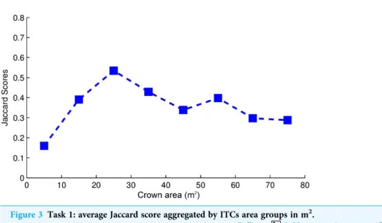
FalsePositive, and FalseNegative. The Jaccard score by crown area is shown inFig. 3. Variability in the crown size influenced the Jaccard score, especially below 40 m2. The detection of small crowns (below 10 m2) had a lower accuracy compared to larger ones
Figure 2 Task 1: plot level overall confusion matrix as a bar chart.TruePositiverepresent the amount of manually delineated ITCs area that was correctly delineated by the automatic delineation method used;
FalsePositiveis the amount of manually deli. Full-size DOI: 10.7717/peerj.6227/fig-2
Figure 3 Task 1: average Jaccard score aggregated by ITCs area groups in m2.
(above 40 m2). In particular, the proposed method showed the best results with crowns of size around 25 m2.
Task 2: alignment
All the test ITCs were aligned with the respectivefield surveyed trees. InFig. 4, the distribution of the test samples according to the two components of the Euclidean distance is shown. As it can be seen on the attributes part of the distance (DATTR), there is high variability (between two and eight m), while for the positional part (DPOS) the value is varying mainly between zero and four m.
Task 3: tree species classification
The overall results for the considered classification task were 88.1% for overall accuracy, 75.7% for kappa accuracy, and 61.5% for mean class accuracy. From the overall
performances, it is clear that the classification method used was effective, as all the performance metrics are quite good, even if the large difference existing among the overall accuracy and the mean class accuracy tells us that the classifier gave priority to the dominant species. Looking atTable 1this is clearly visible. PIPA and QULA classes that represent the majority of the training samples have a producer’s accuracy of 91.1% and 95.5%, respectively, while classes for which the number training samples was low have a low accuracy (i.e., ACRU, PIEL).
Figure 4 Task 2: distribution of the test set samples for the matching part according to the two components of the distance considered in the matching algorithm.
DISCUSSION
Team FEM rankedfirst for ITC delineation (Task 1) of the NEON-NIST challenge. The ITC delineation was carried out on a band of the hyperspectral images, using an approach that was already used in a previous work (Dalponte et al., 2015). The reason for this choice was that, from an initial analysis, the training ITCs provided by the organizers of the NEON-NIST challenge had a poor alignment with the LiDAR data, while they were properly aligned to the hyperspectral data. This fact was confirmed after the end of the challenge, when the organizers revealed that the training and test ITCs were manually delineated on some airborne camera images using a tablet (Marconi et al., 2018). The methods used by the other two teams participating to the challenge (teams Conor and Shawn) and the baseline method were based on LiDAR data (Marconi et al., 2018;
Taylor, 2018;McMahon, 2018), which can explain their poor performances (Jaccard score of 0.184, 0.0555, and 0.0863). The comparison of the results across teams also showed that the FEM approach outperformed the other approaches in the delineation of the small trees, while it was less efficient for the large trees (Marconi et al., 2018). This is due to the fact that we decided to use a small moving window (33 pixels).
Hengl (2006)suggested that in order to detect a circular object on an image (like a tree crown) it is necessary to have at least four pixels representing that object. According to this theory, in our case, using the hyperspectral images at one m resolution allowed us to detect trees with at least four m2of crown size. To this constraint, it should be added that if we used a window size larger than 33 pixels, small trees could have been detected only if they were isolated from other trees. The use of a variable size moving window, like the one that is implemented for LiDAR data in theitcSegment library and used in (Dalponte et al., 2018), would have probably improved thefinal results. In a previous study (Dalponte et al., 2015), the delineation method used in the NEON-NIST competition was compared with three delineation methods based on LiDAR data. The hyperspectral delineation method outperformed the LiDAR based methods on the delineation of broadleaf tree canopies. This fact can also explain the very good performances of team FEM in the NEON NIST data science evaluation challenge Table 1 Task 3: confusion matrix of the tree species classification over the test set, and producer’s and user’s accuracies.
ACRU LIST OTHER PIEL PIPA PITA QUGE QULA QUNI User’s accuracy
ACRU 1 0 1 0 0 0 0 0 0 50 LIST 0 1 0 0 0 0 0 0 0 100 OTHER 1 1 0 0 0 0 1 0 0 0 PIEL 0 0 0 0 2 0 0 0 0 0 PIPA 0 0 0 1 82 0 0 1 0 97.6 PITA 0 0 0 0 4 1 1 0 0 16.7 QUGE 0 0 0 0 0 0 4 0 0 100 QULA 0 0 0 0 2 0 0 21 0 91.4 QUNI 0 0 0 0 0 0 0 0 1 100 Producer’s accuracy 50 50 0 0 91.1 100 66.7 95.5 100
because the study area had many broadleaf trees. Considering these results in the domain of ITC delineation literature it can be said that in general the results are on the average, as it is quite standard to detect 30–40% of the trees in broadleaf forests (Eysn et al., 2015). Comparing the results with others on conifer forests, especially in North Europe, the results appears quite poor, as in spruce forests the accuracy can be over 90% (Vauhkonen et al., 2012).
In the alignment task (Task 2) of the NEON-NIST challenge FEM team ranked in thefirst place, with all the trees correctly matched (score 1). The other participating groups, and the baseline method had a score of 0.48. The baseline prediction was the application of a naive Euclidean distance from thefield tree location to the centroid of the delineated ITC. Team Conor used an approach similar to the one that we used, with a difference in the way the missing data were predicted, and the distance computed (McMahon, 2018). From the results, it seems that a great improvement was made by calculating the missing parameters. Moreover, a visual inspection of the results was essential in correctly aligning all ITC, as two trees were reassigned after this inspection. Such visual inspection is not doable over large datasets, even if, in our experience, it is always suggested as it helps in finding macroscopic errors. As mentioned in the
Introduction, a correct choice of the alignment strategy depends on the type of data that can be used for this purpose. The fact that most of the works in the field of crown delineation use a different arbitrary method is not ideal. Building an alignment strategy common to everyone would simplify methods inter-comparison. In analyzing the literature, it is possible to see that the majority of methods are based either on the overlapping of thefield tree positions with the delineated ITCs (Ene, Næsset & Gobakken, 2012), or on the distance both horizontal (i.e.,XandY) and vertical (e.g., height) (Eysn et al., 2015;Kandare et al., 2017). In many studies a distance constraint, both vertical and horizontal is also applied, meaning that afield surveyed tree and an ITC could be matched only if the distance is lower than a certain value (Kandare et al., 2017). This constraint is usually applied in studies where the matched information is then used for the prediction of stem attributes.
The classification task (Task 3) had the most participants and team FEM ranked in the second place. All the teams properly detected the two-dominant species (PIPA and QULA) while almost all had problems in detecting minority species (i.e., species with a low number of training samples). This is a limitation of many other methods proposed in the literature as many classifiers tend to give priority to highly represented species. Team StanfordCCB that rankedfirst place outperformed team FEM in the detection of PITA and OTHER species while they got the same results for the other species (Marconi et al., 2018). The fact that thefirst three teams in the ranking used an approach of data pre-filtering for either cleaning the training set from noise pixels or to select the most informative features, tells us that this step is quite important, and it should not be avoided. It is worth noting that this dataset is a typical example of an imbalanced dataset, where the ratio between the number of samples of the most frequent class and the number of samples of the least frequent class is very high (PIPA has 49 times samples more than LIST class). Many studies have been done on this problem, especially in the machine
learning community (He & Ma, 2013;Salunkhe & Mali, 2016), and the existing studies can be classified into four groups: (i) data level approaches: these methods aim to rebalance the distribution of classes by applying resampling techniques (e.g., under-sampling or over-sampling) (Chawla et al., 2002); (ii) algorithm level approaches: these methods modify the existing algorithms in order to handle the imbalanced data (Imam, Ting & Kamruzzaman, 2006); (iii) cost sensitive learning approaches: these methods
combines the data and algorithm level approaches to gain benefits of both (Peng, Chan & Fang, 2006); and (iv) classifier Ensemble techniques: these methods combine multiple
diverse classifiers which disagree with each other (Salunkhe & Mali, 2016). All these approaches should be considered in the future in the ecology community as the imbalance of the datasets is quite typical in species classification where it is normal to have a forest with some dominant species and some rare ones.
CONCLUSIONS
In this paper, the results of team FEM of the NEON NIST data science evaluation challenge were presented. The methods applied were effective as team FEM rankedfirst in ITC delineation task (Task 1) and the alignment task (Task 2), and second in the classification task (Task 3). The delineation method proposed was based on hyperspectral images, showing that LiDAR data are not always the best data source for ITC delineation. Importantly, pre-analysis of the available data helped significantly in the choice of the data to use. Alignment was based on both location and tree characteristics, but what probably made the big difference was the way this information was used, and the way the
missing information was predicted. Indeed, another team used the same information obtaining very different results. The classification architecture adopted was quite standard, and it failed to classify rare species. As a future development, it may be interesting to combine both hyperspectral and LiDAR information in the crown delineation, and to consider classifiers especially developed for imbalanced data problems that can improve the classification of rare species.
ADDITIONAL INFORMATION AND DECLARATIONS
FundingThe National Ecological Observatory Network is a program sponsored by the National Science Foundation and operated under cooperative agreement by Battelle Memorial Institute. This material is based in part upon work supported by the National Science Foundation through the NEON Program. The ECODSE competition was supported, in part, by a research grant from NIST IAD Data Science Research Program to Daisy Zhe Wang, Ethan White, and Stephanie Bohlman, by the Gordon and Betty Moore
Foundation’s Data-Driven Discovery Initiative through grant GBMF4563 to Ethan White, and by an NSF Dimension of Biodiversity Program grant (DEB-1442280) to Stephanie Bohlman. There was no additional external funding received for this study. The funders had no role in study design, data collection and analysis, decision to publish, or
Grant Disclosures
The following grant information was disclosed by the authors:
National Science Foundation and operated under cooperative agreement by Battelle Memorial Institute.
National Science Foundation through the NEON Program. NIST IAD Data Science Research Program.
Gordon and Betty Moore Foundation’s Data-Driven Discovery Initiative: GBMF4563. NSF Dimension of Biodiversity program: DEB-1442280.
Competing Interests
The authors declare that they have no competing interests. Author Contributions
Michele Dalponte conceived and designed the experiments, performed the experiments, analyzed the data, contributed reagents/materials/analysis tools, preparedfigures and/or tables, authored or reviewed drafts of the paper, approved thefinal draft.
Lorenzo Frizzera performed the experiments, analyzed the data, contributed reagents/ materials/analysis tools, approved thefinal draft.
Damiano Gianelle conceived and designed the experiments, contributed reagents/ materials/analysis tools, authored or reviewed drafts of the paper, approved thefinal draft.
Data Availability
The following information was supplied regarding data availability:
ECODSE group. (2017). ECODSE competition training set [Data set]. Zenodo.
http://doi.org/10.5281/zenodo.867646.
REFERENCES
Aasen H, Burkart A, Bolten A, Bareth G. 2015.Generating 3D hyperspectral information with lightweight UAV snapshot cameras for vegetation monitoring: from camera calibration to quality assurance.ISPRS Journal of Photogrammetry and Remote Sensing108:245–259
DOI 10.1016/j.isprsjprs.2015.08.002.
Bruzzone L, Roli F, Serpico SB. 1995.An extension to multiclass cases of the Jeffreys-Matusita distance.IEEE Transactions on Geoscience and Remote Sensing33:1318–1321.
Chawla NV, Bowyer KW, Hall LO, Kegelmeyer WP. 2002.SMOTE: synthetic minority over-sampling technique.Journal of Artificial Intelligence Research16:321–357
DOI 10.1613/jair.953.
Clark ML, Roberts DA, Clark DB. 2005.Hyperspectral discrimination of tropical rain forest tree species at leaf to crown scales.Remote Sensing of Environment96(3–4):375–398
DOI 10.1016/j.rse.2005.03.009.
Coomes DA, Dalponte M, Jucker T, Asner GP, Banin LF, Burslem DFRP, Lewis SL, Nilus R, Phillips OL, Phua M-H, Qie L. 2017.Area-based vs tree-centric approaches to mapping forest carbon in Southeast Asian forests from airborne laser scanning data.Remote Sensing of Environment194:77–88DOI 10.1016/j.rse.2017.03.017.
Dabboor M, Howell S, Shokr M, Yackel JJ. 2014.The Jeffries–Matusita distance for the case of complex Wishart distribution as a separability criterion for fully polarimetric SAR data.
International Journal of Remote Sensing35(19):6859–6873.
Dalponte M. 2018.itcSegment: individual tree crowns segmentation.Available at
https://cran.r-project.org/web/packages/itcSegment/.
Dalponte M, Bruzzone L, Gianelle D. 2008.Fusion of hyperspectral and LIDAR remote sensing data for classification of complex forest areas.IEEE Transactions on Geoscience and Remote Sensing46(5):1416–1427DOI 10.1109/TGRS.2008.916480.
Dalponte M, Bruzzone L, Gianelle D. 2012.Tree species classification in the Southern Alps based on the fusion of very high geometrical resolution multispectral/hyperspectral images and LiDAR data.Remote Sensing of Environment123:258–270DOI 10.1016/j.rse.2012.03.013.
Dalponte M, Bruzzone L, Vescovo L, Gianelle D. 2009.The role of spectral resolution and classifier complexity in the analysis of hyperspectral images of forest areas.Remote Sensing of Environment113(11):2345–2355DOI 10.1016/j.rse.2009.06.013.
Dalponte M, Frizzera L, Ørka HO, Gobakken T, Næsset E, Gianelle D. 2018.Predicting stem diameters and aboveground biomass of individual trees using remote sensing data.
Ecological Indicators85:367–376DOI 10.1016/j.ecolind.2017.10.066.
Dalponte M, Ørka HO. 2016.varSel: sequential forwardfloating selection using jeffries-matusita distance.Available athttps://cran.r-project.org/web/packages/varSel/.
Dalponte M, Ørka HO, Ene LT, Gobakken T, Næsset E. 2014.Tree crown delineation and tree species classification in boreal forests using hyperspectral and ALS data.Remote Sensing of Environment140:306–317DOI 10.1016/j.rse.2013.09.006.
Dalponte M, Orka HO, Gobakken T, Gianelle D, Naesset E. 2013.Tree species classification in boreal forests with hyperspectral data.IEEE Transactions on Geoscience and Remote Sensing
51(5):2632–2645DOI 10.1109/TGRS.2012.2216272.
Dalponte M, Reyes F, Kandare K, Gianelle D. 2015.Delineation of individual tree crowns from ALS and hyperspectral data: a comparison among four methods.European Journal of
Remote Sensing48(1):365–382DOI 10.5721/EuJRS20154821.
Duncanson LI, Dubayah RO, Cook BD, Rosette J, Parker G. 2015.The importance of spatial detail: Assessing the utility of individual crown information and scaling approaches for lidar-based biomass density estimation.Remote Sensing of Environment168:102–112
DOI 10.1016/j.rse.2015.06.021.
Ene L, Næsset E, Gobakken T. 2012.Single tree detection in heterogeneous boreal forests using airborne laser scanning and area-based stem number estimates.International Journal of Remote Sensing33(16):5171–5193DOI 10.1080/01431161.2012.657363.
Eysn L, Hollaus M, Lindberg E, Berger F, Monnet J-M, Dalponte M, Kobal M, Pellegrini M, Lingua E, Mongus D, Pfeifer N. 2015.A benchmark of lidar-based single tree detection methods using heterogeneous forest data from the alpine space.Forests6(12):1721–1747
DOI 10.3390/f6051721.
Fassnacht FE, LatifiH, Sterenczak K, Modzelewska A, Lefsky M, Waser LT, Straub C, Ghosh A. 2016.Review of studies on tree species classification from remotely sensed data.
Remote Sensing of Environment186:64–87DOI 10.1016/j.rse.2016.08.013.
Ferraz A, Bretar F, Jacquemoud S, Gonçalves G, Pereira L, Tomé M, Soares P. 2012.
3-D mapping of a multi-layered Mediterranean forest using ALS data.Remote Sensing of Environment121:210–223DOI 10.1016/j.rse.2012.01.020.
Foody GM, Hill RA. 1996.Classification of tropical forest classes from Landsat TM data.
Franklin J, Logan T, Woodcock C, Strahler A. 1986.Coniferous forest classification and inventory using landsat and digital terrain data.IEEE Transactions on Geoscience and Remote SensingGE-24(1):139–149DOI 10.1109/TGRS.1986.289543.
Gomes MF, Maillard P, Deng H. 2018.Individual tree crown detection in sub-meter satellite imagery using Marked Point Processes and a geometrical-optical model.Remote Sensing of Environment211:184–195DOI 10.1016/j.rse.2018.04.002.
Gómez-Chova L, Calpe J, Camps-Valls G, Martín-Guerrero J, Olivas E, Vila-Francés J, Alonso L, Moreno J. 2003.Feature selection of hyperspectral data through local correlation and SFFS for crop classification. In:IEEE International Geoscience and Remote Sensing Symposium. Proceedings (IEEE Cat. No.03CH37477). Piscataway: IEEE, 555–557.
He H, Ma Y. 2013.Imbalanced learning: foundations, algorithms, and applications. Hoboken: John Wiley & Sons, Inc.
Hengl T. 2006.Finding the right pixel size.Computers & Geosciences32(9):1283–1298
DOI 10.1016/j.cageo.2005.11.008.
Hung C, Bryson M, Sukkarieh S. 2012.Multi-class predictive template for tree crown detection.
ISPRS Journal of Photogrammetry and Remote Sensing68:170–183
DOI 10.1016/j.isprsjprs.2012.01.009.
Imam T, Ting KM, Kamruzzaman J. 2006.z-SVM: An SVM for improved classification of imbalanced data. In: Sattar A, Kang B, eds.AI 2006: Advances in Artificial Intelligence. AI 2006. Lecture Notes in Computer Science,Vol. 4304. Berlin, Heidelberg: Springer, 264–273.
Kandare K, Ørka HO, Dalponte M, Næsset E, Gobakken T. 2017.Individual tree crown approach for predicting site index in boreal forests using airborne laser scanning and hyperspectral data.International Journal of Applied Earth Observation and Geoinformation
60:72–82DOI 10.1016/j.jag.2017.04.008.
Karatzoglou A, Smola A, Hornik K, Zeileis A. 2004.kernlab—An S4 Package for Kernel Methods in R.Journal of Statistical Software11(9):1–20DOI 10.18637/jss.v011.i09.
Ke Y, Quackenbush LJ. 2011.A review of methods for automatic individual tree-crown detection and delineation from passive remote sensing.International Journal of Remote Sensing
32(17):4725–4747DOI 10.1080/01431161.2010.494184.
Lee AC, Lucas RM. 2007.A LiDAR-derived canopy density model for tree stem and crown mapping in Australian forests.Remote Sensing of Environment111(4):493–518
DOI 10.1016/j.rse.2007.04.018.
Lindberg E, Holmgren J. 2017.Individual tree crown methods for 3D data from remote sensing.
Current Forestry Reports3(1):19–31DOI 10.1007/s40725-017-0051-6.
Marconi S, Graves SJ, Gong D, Nia MS, Bras M Le, Dorr JB, Fontana P, Gearhart J,
Greenberg C, Harris DJ, Arvind Kumar S, Nishant A, Prarabdh J, Rege SU, Bohlman SA, White EP, Wang DZ. 2018.A data science challenge for converting airborne remote sensing data into ecological information.PeerJ Preprints6:e26966v1.
McMahon CA. 2018.NEON NIST data science evaluation challenge: methods and results of team Conor.PeerJ Preprints6:e26977v1DOI 10.7287/peerj.preprints.26977v1.
Padma S, Sanjeevi S. 2014.Jeffries Matusita-Spectral Angle Mapper (JM-SAM) spectral matching for species level mapping at Bhitarkanika, Muthupet and Pichavaram mangroves.
ISPRS—International Archives of the Photogrammetry, Remote Sensing and Spatial Information SciencesXL-8:1403–1411DOI 10.5194/isprsarchives-XL-8-1403-2014.
Peng Li, Chan KL, Fang W. 2006.Hybrid kernel machine ensemble for imbalanced data sets. In:18th International Conference on Pattern Recognition (ICPR’06). Piscataway: IEEE, 1108–1111DOI 10.1109/ICPR.2006.643.
Popescu SC, Wynne RH, Nelson RF. 2003.Measuring individual tree crown diameter with lidar and assessing its influence on estimating forest volume and biomass.Canadian Journal of Remote Sensing29(5):564–577DOI 10.5589/m03-027.
Pudil P, Novovičová J, Kittler J. 1994.Floating search methods in feature selection.Pattern Recognition Letters15(11):1119–1125DOI 10.1016/0167-8655(94)90127-9.
R Development Core Team. 2008.R: a language and environment for statistical computing. Vienna: R Foundation for Statistical Computing.Available athttp://www.R-project.org/.
Real R, Vargas JM. 1996.The probabilistic basis of jaccard’s index of similarity.Systematic Biology
45(3):380–385DOI 10.1093/sysbio/45.3.380.
Richards JA, Jia X. 2006.Remote sensing digital image analysis. Berlin, Heidelberg: Springer.
Salunkhe UR, Mali SN. 2016.Classifier ensemble design for imbalanced data classification: a hybrid approach.Procedia Computer Science85:725–732DOI 10.1016/j.procs.2016.05.259.
Taylor S. 2018.NEON NIST data science evaluation challenge: methods and results of team Shawn.PeerJ Preprints6:e26967v1DOI 10.7287/peerj.preprints.26967v1.
Tuominen J, Lipping T. 2016.Spectral characteristics of common reed beds: studies on spatial and temporal variability.Remote Sensing8(3):181DOI 10.3390/rs8030181.
Vauhkonen J, Ene L, Gupta S, Heinzel J, Holmgren J, Pitkänen J, Solberg S, Wang Y, Weinacker H, Hauglin KM, Lien V, Packalén P, Gobakken T, Koch B, Næsset E, Tokola T, Maltamo M. 2012.Comparative testing of single-tree detection algorithms under different types of forest.Forestry85(1):27–40DOI 10.1093/forestry/cpr051.
Yu B, Ostland IM, Gong P, Pu R. 1999.Penalized discriminant analysis of in situ hyperspectral data for conifer species recognition.IEEE Transactions on Geoscience and Remote Sensing