A Pareto-based Evolutionary Algorithm using
Decomposition and Truncation for Dynamic
Multi-objective Optimization
Junwei Oua,b, Jinhua Zhenga,c,∗, Gan Ruand, Yaru Hua, Juan Zoua, Miqing
Lid, Shengxiang Yange, Xu Tanb,∗
a
Key Laboratory of Intelligent Computing and Information Processing, Ministry of Education, Information Engineering College of Xiangtan University, Xiangtan, Hunan
Province, China
b
School of Software Engineering, Shenzhen Institute of Information Technology, Shenzhen 518172, China
c
Hunan Provincial Key Laboratory of Intelligent Information Processing and Application, Hengyang Normal University, Hengyang, 421002, China
d
School of Computer Science, University of Birmingham, Birmingham B15 2TT, U. K.
e
School of Computer Science and Informatics, De Montfort University, Leicester LE1 9BH, U.K.
Abstract
Maintaining a balance between convergence and diversity of the population in the objective space has been widely recognized as the main challenge when solving problems with two or more conflicting objectives. This is added by an-other difficulty of tracking the Pareto optimal solutions set(POS) and/or the Pareto optimal front(POF) in dynamic scenarios. Confronting these two issues, this paper proposes a Pareto-based evolutionary algorithm using decomposition and truncation to address such dynamic multi-objective optimization problem-s (DMOPproblem-s). The propoproblem-sed algorithm includeproblem-s three contributionproblem-s: a novel mating selection strategy, an efficient environmental selection technique and an effective dynamic response mechanism. The mating selection considers the decomposition-based method to select two promising mating parents with good diversity and convergence. The environmental selection presents a modified
∗Corresponding author
Email addresses: [email protected](Junwei Ou),[email protected](Jinhua Zheng),
[email protected](Gan Ruan),[email protected](Yaru Hu),
[email protected](Juan Zou),[email protected](Miqing Li),[email protected] (Shengxiang Yang),[email protected](Xu Tan)
truncation method to preserve good diversity. The dynamic response mecha-nism is evoked to produce some solutions with good diversity and convergence whenever an environmental change is detected. In the experimental studies, a range of dynamic multi-objective benchmark problems with different charac-teristics were carried out to evaluate the performance of the proposed method. The experimental results demonstrate that the method is very competitive in terms of convergence and diversity, as well as in response speed to the changes, when compared with six other state-of-the-art methods.
Keywords:
Dynamic multi-objective optimization, Evolutionary algorithms, Decomposition, Diversity
1. Introduction
Over the past decades, evolutionary multi-objective optimization (EMO) has been of interest to researchers due to the inherent characteristics of evolutionary algorithms (EAs) when addressing problems with no less than two conflicting goals. Specifically, EAs are able to find a set of trade-off solutions that
ap-5
proximate to the POF. Therefore, multi-objective optimization evolutionary algorithms (MOEAs) have been widely applied in many real-world engineering scenarios [1]. The main challenge for MOEAs in dealing with multi-objective optimization problems (MOPs) is determining how to balance diversity and
convergence1during the optimization process.
10
A particular kind of real-life MOPs, called dynamic multi-objective opti-mization problems (DMOPs), have objective functions, constraints and/or pa-rameters that may be time variant [2]. DMOPs pose considerable challenges to optimization algorithms due to the dynamism of various problems [3][4][5]. Moreover, the change frequency and change severity are two important
param-15
1Convergence and diversity in the paper refer to the objective space, except where explicitly
eters that play an important role in influencing the performance of DMOEAs [3][6]. The change frequency [2] defines the number of generations from one environmental change to the next. High severity of change [2] requires algo-rithms that have good ability to search because when the POS changes in the dynamic environment, the population may lose the ability to trace the changing
20
POS. Even though MOEAs have great advantages for solving MOPs, they also have limitations in solving these problems. The reason is that the values of the objective functions may vary when there are environmental changes. Thus, MOEAs are supposed to be greatly improved to quickly find the POS or POF before the next environmental change [7][8] comes. In recent years, dynamic
25
multi-objective evolutionary algorithms (DMOEAs) have been extensively ap-plied in many areas, such as scheduling [9][10], control [11][12][13], planning [14][15][16][17][18], design [19] and machine learning [20]. Although traditional MOEAs [21][22][23] dealing with MOPs can accelerate the converging speed of the population, one drawback in solving DMOPs is that they sometimes lack
30
adequate diversified solutions to help the population jump out of the current optimum.
Additionally, detection of whether a change has occurred is a critical part during the evolutionary process. Reevaluating solutions [9][3][8][24][7][6] and checking the population’s statistical information [2][25][26] are two main ways
35
to detect a change. The approach of reevaluating solutions is employed by reevaluating members at every generation. Although this approach is easy to implement, it needs additional function evaluations. Checking the population’s statistical information is a good way as it doesn’t need function
evaluation-s. However, it can cause false positives for detector changeevaluation-s. Jiang et al. [4]
40
introduced a steady-state manner to detect changes. In the manner, the popula-tion’s individuals are checked in random order one by one to determine whether a discrepancy exists between their previous objective values. If a discrepancy is found, the change is successfully detected and the rest of the population’s mem-bers do not need to be checked. However, the population memmem-bers also need
45
selected to detect the environmental change. Moreover, less detectable environ-mental changes [27] pose a big challenge for DMOEAs. We can not deal with such issues now and leave it as one of our future works. The main contributions of this study are summarized as follows.
50
1. An effective mating selection method was developed to select well con-verged and diversified parents, and the main goal was to generate good offsprings.
2. In environmental selection process, an improved truncation method was to improve the diversity of whole population.
55
3. In order to quickly react to environmental change, a good change response mechanism based an exploration strategy and an exploitation strategy was designed.
The paper is structured as follows. Section 2 describes some basic defini-tions, related works and motivation. Section 3 presents the proposed algorithm
60
in detail. Section 4 presents the experimental setting for comparison. Section 5 gives experimental results and a comparison of the algorithm to other algo-rithms. A further discussion of the algorithms is offered in Section 6. Finally, conclusions are drawn in Section 7.
2. Background
65
2.1. Dynamic Multi-objective Optimization
In this paper, we consider that minimization problems and DMOPs [2][28] can be presented as follows:
minF(x, t) = (f1(x, t), f2(x, t), ...fm(x, t))T, s.t.g(x, t)≤0, h(x, t) = 0, x∈[L, U], (1)
where t represents the time variable, and x = (x1, x2, ..., xn)T is the decision
variable vector. [L,U] = {x=(x1, ..., xn)|li ≤ xi ≤ ui, i = 1,2, .., n} is the
decision space, where L = (l1, ..., ln)T and U = (u1, ..., un)T are the lower and
upper bounds, respectively. F= (f1, f2, ..., fm)T is the m-dimensional objective
vector and g(x,t)≤0 and h(x,t) = 0 are the inequality and equality constraints.
The definition of DMOPs is a standard formula proposed by Farinaet al. [2]
and the formula is used in most literature [28][4]. Thus, constrained DMOPs
75
are not considered in this paper. The time variable, t, is associated with the generation number of the EA; t is calculated as follows [2][5]:
t= 1
nt ⌊τ
τt
⌋, (2)
where τ is the generation number, nt is change severity and τt is change
fre-quency.
Definition 1. Pareto Dominance [21]: Assume that p and q are any two
in-80
dividuals in the population; pis said to dominateq, written as f(p)≺f(q) if
fi(p)≤fi(q)∀i∈1,2, ..., mandfj(p)< fj(q)∃j∈1,2, ..., m.
Definition 2. Pareto Optimal Set (POS):xis the decision vector; Ω is the
de-cision space;F is the objective function. A solution is said to be nondominated
if it is not dominated by any other solutions in Ω. Thus, the POS [2][29] is the
85
set of all nondominated solutions and can be defined mathematically as follows:
P OS:={x∈Ω|¬∃x∗∈Ω, F(x∗)≺F(x)}. (3)
Definition 3. Pareto Optimal Front (POF): xis the decision vector; Ω is the
decision space; F is the objective function. Thus, the POF is the set of all
nondominated solutions with respect to the objective space and can be defined mathematically as follows:
90
P OF :={y=F(x)|x∈P OS}. (4)
Due to the dynamic change of the POS and POF, Farinaet al. [2] classified
DMOPs into four different types.
• T ype II: Both theP OS andP OF change with time.
• T ype III: TheP OSremains fixed, while theP OF changes with time.
95
• T ype IV: Both theP OSandP OF remain fixed.
We mainly deal with the first three types of changes in dynamic multi-objective
optimization, although the TypeIV change may also occur in some cases.
2.2. Related Works
Many DMOEAs have been proposed in recent years and existing approaches
100
[30][5] can be classified into the following categories: convergence-based method-ologies, diversity-based methodmethod-ologies, and other methodologies [31][6] accord-ing to their ways of managaccord-ing dynamics [4].
As its name suggests, convergence-based approaches are used to improve the convergence of the population, so as to guide the population to converge to
105
the next POF. Current convergence-based methods mainly include the memory strategy and prediction technique. Memory approaches [7][32][33][34] memo-rize the previously obtained POS to track the new POS when the environment has regularities. The memory approaches record past historical information to
quickly respond to the new environmental change. Peng et al. [34] proposed
110
a memory strategy that preserves some promising solutions. When the envi-ronment changes, the method usually selects some nondominated solutions and stores them in a memory pool. Because these elite individuals in memory pool are optimal with best convergence and diversity in past environment. Thus, the approach can increase diversity to some extent. After that, these elite
solu-115
tions are selected by nondominated selection, and are reused to adapt the new environment. While it is critical to accelerate convergence of the population, for non-periodic problems or the early stages of periodic problems, memory approaches are not as effective as we wish.
Prediction-based mechanisms always apply past population information to
120
forecast some information of the next population and re-initialize the population through certain prediction models. An appropriate prediction model is rather
essential for the accuracy and effectiveness of the prediction strategy whenever there is an environmental change. Prediction approaches can provide a guiding direction for the evolution of the population towards the POF. In 2006,
Hatza-125
kiset al. [32] proposed a feed-forward prediction strategy (FPS). In 2013, Zhou
et al. [3] proposed a population prediction strategy (PPS). FPS and PPS use the autoregressive model to predict population, which is effective in solving D-MOPs in some degree. However, there are some difficulties for FPS in solving these DMOPs which have a nonlinear correlation between decision variables.
130
This is because FPS only predicts the boundary points of the population, which can not reflect the whole population. In addition, because of the lack of his-torical information accumulation, PPS has low convergence in the early stage.
Murugananthamet al. [35] proposed a prediction model based on the Kalman
Filter (MOEA/D-KF). The MOEA/D-KF technique involves a prediction step
135
and a measurement step estimates the current state a priori. In the subsequent measurement, a priori estimate from the MOEA/D-KF is updated to obtain a posteriori. It is applied to the whole population to direct the search towards the next POS instead of the expansion or contraction of the POS or POF mani-fold. The large prediction errors result in the poor performance of the obtained
140
solutions.
Diversity-based techniques can be classified into two categories according to the period of enhancing the diversity, which are diversity introduction and diver-sity preservation. Diverdiver-sity introduction is recognized as the response technique to the environmental changes. Specifically, whenever there is an environmental
145
change, diversity introduction is evoked to generate some diversified solutions to increase the diversity of the population. For example, hyper-mutation method-s [36][8][37][38] and random producing method-solutionmethod-s [8][12][25] are commonly umethod-sed to help the population escape from the current positions. Additionally, other modified diversity maintenance strategies [39][40] have been adopted to improve
150
the population’s diversity. On the other hand, diversity preservation is not usu-ally designed to explicitly react the changes of environment; instead it mainly focuses on the innate diversity preservation of the optimization algorithms. In
dCOEA[7], a multipopulation method is proposed to enhance the population diversity in a competitive and cooperative way. In DTAEA[30], a dynamic
two-155
archive EA is developed to maintain two co-evolving populations, which have complementary effects on enhancing the population diversity. Properly increas-ing the population’s diversity can make the converged population jump out of the current optimum when the environmental change is detected. Appropriate diversity enhancement is essential and rewarding for algorithms to track the
160
changing environment, whereas excessive diversity strengthening may result in low convergence of the algorithms. Based on this idea, many DMOEAs have been proposed, such as co-evolutionary algorithms [7], memetic computing [14], the modeling approach [5] and other methods [38][41][29][42][43].
Aside from the aforementioned approaches, the Particle swarm optimizer
165
(PSO) can deal with MOPs. Proposed by Kennedyet al. [44], PSO is composed
of plenty of particles. PSO also has good performance with DMOPs. Helbiget
al. [31] introduced a dynamic Vector Evaluation Particle Swarm Optimisation
(DVEPSO) algorithm to solve DMOPs. Due to outdated memory and diversity loss, PSO easily moves into local optima when the environmental change is
170
detected. Ant colony optimisation (ACO) is an optimization algorithm based on the natural behavior of ants. It has the ability to deal with multi-objective problems due to its flexibility in being able to add multiple colonies, or multiple pheromone and heuristic matrices. ACO also can be applied to DMOPs because it has the ability to retain useful information when an environmental change
175
occurs. Eatonet al. [45][46][47] proposed some approaches based on ACO to
cope with a dynamic railway junction rescheduling problem. They found that ACO has a role to play in a dynamically changing environment and it can deal with real-world dynamic problems.
2.3. Motivation 180
Multi-objective evolutionary algorithm based on decomposition (MOEA/D) [23] is a competent aggregation-based methodology in the community of EMO. Numerous studies have been conducted to improve the quality of MOEA/D in
static EMO in recent years. Nevertheless, there is little research that relies on improvements of MOEA/D to address DMOPs. Additionally, as already
185
mentioned, current studies on EMO mainly focus on either introducing the diversity to react to environmental changes or maintaining the diversity during the process of optimization. Not many investigations have been explicitly carried out to enhance diversity during the period when searching and reacting occur simultaneously.
190
In this paper, we put forward a novel Pareto-based evolutionary algorithm using decomposition and truncation (PDTEA) to handle DMOPs. In PDTEA, the decomposition-based algorithm is first adapted to enhance the diversity of the whole population during the optimization process. Then the aggregation functions [23] and Pareto-dominance [21] relationship are used to improve the
195
convergence speed of the population. On the basis of these two steps, a new mat-ing selection strategy, an effective environmental selection technique and a mech-anism to handle change in the environment are proposed. The decomposition-based approach is used to select two well-converged and well-diversified mating parents during the mating selection. In addition, an improved truncation
op-200
eration [22] is adopted during environmental selection for density estimation [22][48][49]. If a change is detected, the mechanism to handle changes uses t-wo strategies including an exploration strategy and an exploitation strategy to adapt to the new environment. The first strategy is to explore an individual of the population based on the direction of the individual and its nearest individual
205
which can search for good solutions in the area. The exploitation strategy uses individual variation to enhance convergence. We can use historical information to guide evolution for periodic problems. For each generation, PDTEA select-s the beselect-st select-solutionselect-s in each select-subregion to generate new select-solutionselect-s to accelerate convergence. In the environmental selection, an improved truncation procedure
210
from that of SPEA2 [22] is used to preserve a good distribution of the population for the next generation.
3. Proposed Algorithm
In this section, the decomposition-related preparatory procedure is described first. In order to handle DMOPs, determining how to select efficiently
mat-215
ing parents producing offsprings and preserving good solutions are critical to DMOAs. Thus, a procreation procedure and environmental selection are pro-posed. Furthermore, a mechanism to handle changes is introduced and we present an overall framework for the proposed algorithm. Finally, we analyze the computational complexity of the compared algorithms and PDTEA.
220
3.1. Decomposition-related preparatory procedures
Given that decomposition-based methodologies are designed to be applied to the evenly distributed reference points in the objective space to ensure diversity
before the evolution, a set of reference points w = (w1, ..., wM)T is produced
through a systematic approach [50][51][52], wherewi ≥0 for all i∈ {1, ..., M};
225
M is is the number of objectives, and PM
i=1wi=1. The reference points are
evenly distributed on anM−1-dimension unit simplex, which is a normalized
hyperplane. The required generated number of reference points H is closely
related to the number of considered divisions along each objectivep, which can
be denoted by the following formula:
230 H = M +p−1 p , (5)
whereM is the number of objectives.
Thereafter, the initialization populationP0 is normalized in the hyperplane
in which the set of reference points is located. First, the ideal point zmin =
(zmin1 , zi
min, ..., zMmin)T and the worst point zmax = (zmax1 , zmaxi , ..., zMmax)T of
the population P0 are calculated respectively, where zmini and zimax are the
235
smallest and the biggest value of the i-th objective in the objective space. Thus, the normalized member x can be calculated as follows [49]:
ˆ fi(x) = fi(x)−zmini zi max−zmini , (6)
where ˆfi(x) denotes the i-th normalized objective of member x. Thus, the
objective vector of the normalized individual x in the population can be denoted as ( ˆf1(x),fˆi(x), ...,fˆM(x))T, where x∈P0.
240
There are several reputable aggregation functions in MOEA/D which convert a multi-objective problem vector into a scalar optimization problem. The first approach is called the Weighted Sum Approach [23]. Its scalar optimization function can be presented as follows:
g(x|w) =
M X
i=1
wifi(x), (7)
The solution with the minimization value ofg(x|w) is regarded as the best
solu-245
tion with the best convergence within the reference pointw= (w1, w2, .., wM)T.
The second approach is the Tchebycheff Approach [23] defined as follows:
g(x|w) = min
1≤i≤M{wi|fi(x)−z
i
min|}, (8)
The third approach is the Penalty-based Boundary Intersection Approach(PBI) [23], presented as follows: g(x, zmin) =d1+θd2, (9) whered1= ||(f(x)−zmin) T w|| ||w|| andd2=||f(x)−(zmin+d1 w ||w||)||. 250
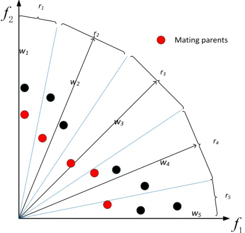
Afterwards, each individual in the population is associated with the reference directions that are generated through reference points and the origin. The
refer-ence directions are meant to divide the population intoN subregions. For each
normalized individual in the population, the perpendicular distance between it and the reference directions is computed. The individual is associated with the
255
reference direction which has the smallest perpendicular distance. This is illus-trated in Fig.1. Each individual associated with the reference direction is given an aggregation function value [52] through one specific aggregation function [23].
3.2. Procreation procedure
The procreation procedure is adopted to produce offspring individuals from
260
f
f
r1 r2 r3 r4 r5Mating parents
w
1w
3w
4w
5w
2Figure 1: Association of population members and matching selection selection and generating offspring. The former is to select two mating parents using a specific strategy. Generating offspring, as its name suggests, is used to produce offspring solutions through genetic operators from the chosen mating parents. To enhance the diversity of the population, different from the original
265
MOEA/D, which selects two mating parents from the neighborhood, the pro-posed mating selection randomly chooses two parents from the N subregions. After computing the aggregation function values of the individuals associated with the same reference direction, the solution with the best aggregation func-tion value is selected as one of the mating parents. Another mating parent is
270
in PDTEA improves the convergence of the algorithm because individuals with the best aggregation function values are selected as mating parents to produce solutions with good convergence. Considering the association regulation, it is likely that some reference directions have several associated individuals or no
275
individuals. If the chosen subregion does not have associated solutions, it will never be selected. For another situation, when all individuals are only in a subregion, parent individuals are randomly selected by the binary tournament selection [21] from the population.
Then, the offspring generation procedure, using the mating parents to
pro-280
duce the offspring population through the genetic operator, is followed as the mating selection. As for the operator of genetics, in theory, any can be selected to achieve the operator of genetics. In this paper, the simulated binary crossover (SBX) [21] and polynomial mutation (PM) [21] are used as the crossover oper-ator and mutation operoper-ator, respectively. The details of the procreation
proce-285
dure are shown in Algorithm 1.
3.3. Environmental selection
The environmental selection is designed to preserve the good solutions of the convergence and diversity performance after the reproduction procedure. The process of environmental selection is presented as follows. The
Pareto-290
domination relationship has been proved to be an effective approach to cope with MOPs with two or three goals. Given that most existing DMOPs are problems with no more than three objectives, the non-dominated sort in NSGA-II [21] is first conducted on the combination of the parent and offspring population, after which all the solutions in the union are compared with each other to find
295
the non-dominated levels (i.e.,F1, ..., Fl, ..., where l≤N ), where each solution
belongs to [21]. Then, each nondomination level fromF1 is included in a new
populationP until the size ofP equals to, or first time exceeds the predefined
threshold.
In the so-called critical layer Fl, in order to maintain the diversity of the
300
Algorithm 1Procreation procedure Input:
N, P(parent population) Output:
R(offspring population), Q(combination of parent and offspring)
1: Compute the normalized objective vector of parent population by Eq. 6
2: Associate each member in the normalized parent population with the
refer-ence direction and decompose the objective space into N subregion.
3: Give an aggregation function value of each member in each subregion by
one specific aggregation function [23] and find the member of the smallest aggregation function value in each subregion.
4: fori: = 1 to Ndo
5: Randomly select two individuals with good aggregation function value
fromN subregions as the mating parents.
6: Generate a new solution using the chosen parents through SBX and PM
[21].
7: end for
8: Combine parent and offspring into Q.
SPEA2 [22]. The nearest Euclidean distance of the individuals in the critical
layerFl to individuals of selected new populationP is computed as follows:
d(q, P) = min
p∈P||f(q)−f(p)||, (10)
where q ∈ Fl. Then, the distance of Fl is sorted and the individuals of Fl
with bigger distance are selected for population P. In this way, the whole
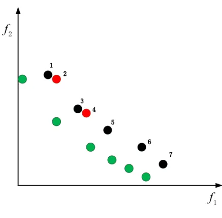
305
population’s diversity is maintained instead of only in the critical layer. Fig. 2 gives an example to illustrate the reason. Assume that the green points represent
the individuals ofF1, the red and black points belong to the critical layerF2.
Assume that two individuals of F2 need to be selected. In order to improve
the whole population’s diversity, the red points with the bigger distance are
310
f
f
Figure 2: Truncation operation.
3.4. Dynamic response mechanism
In order to cope with the two challenges of DMOPs, that is tracing the chang-ing POS and enhancchang-ing diversity, in the period of environmental response, this paper proposes a dynamic response strategy based on exploration and
exploita-315
tion [29][34]. Exploration guides the whole population to evolve to the region of the next environmental change. Exploitation is applied to adequately search the region that has been located with a local search approach to find more solutions with good convergence and diversity in the decision space.
The exploration strategy is to explore the possible area in which the new
320
population may situate and maintain the diversity of the population to some degree. The direction of individuals can help to guide the convergence of the
population and improve diversity in the decision space. Suppose that xi
Algorithm 2Environmental selection Input:
N(population size), Q(combination of parent and offspring) Output: P(new population) 1: {F1, F2, ...Fl, ...} ← NonDominatedSorting(Q). 2: while|P|+|Fi| ≤Ndo 3: P←P∪Fi, i←i+1; 4: end while
5: Calculate the distance of individual ofFl using Eq. 10.
6: Individuals ofFl are sorted by distance and we add individuals ofFl with
bigger distance to population p.
(xi1
t , xit2, ..., xint )(i= 1,2, ...N) is the i-th individual population at timet, where
N is the population size. For each individual xt in population t, there is an
325
individual in populationt-1 (Pt−1) having the nearest distance toxt, which can
be found using the following equation:
xjt−1=arg min
y∈Pt−1
ky−xitk2, j= 1,2, ..., N (11)
where y is an individual of population at time t-1. Then, the direction of the
i-th individual at timet is defined as follows:
Dti=xit−xjt−1, (12)
Then, a varianceσt is defined as:
330 σt= N min i=1 kD i tk, i= (1,2, ...N) (13) where k Di
t k is the length of the the i-th individual’s direction and σt is the
minimum length of the individuals’ direction. Then individuals at time t + 1 are generated by the individuals of time t, the moving direction of each individual and the variance according to the following formula:
xi
x
x
tP
-tP
3RLQWVRIH[SORUDWLRQ 'LUHFWLRQRIWKHLQGLYLGXDO )LQGWKHQHDUHVWLQGLYLGXDOIRUPtFigure 3: Exploration of the individual.
whereN(0,σt) is a random number generated by a Gaussian distribution with
335
a mean of zero and standard deviantion of σt. Fig. 3 gives the explanation
of how to explore individuals. First, the responding nearest individual ofxi
t in
Pt−1is found according to Eq. 11 and then the direction of each individual and
the defined variance in terms of Eq. 12 and Eq. 13 are computed. Lastly, N
individuals are generated by means of Eq. 14. The main steps of the exploration
340
strategy are described in Algorithm 3.
After exploring the region of the new POS, another strategy using local
search is used to exploit the area around the present POS. First, vectordj =
(d1j, d2j, ..., dnj) is defined, then the distances between individualxij and the low
and upper boundary are calculated, anddjirepresenting the smaller distance is
denoted as:
dji=min{|xji−li|,|xji−ui|}, (15)
wherej = 1,2,...,N;i = 1, 2,..., n;li andui are the low and upper boundaries,
respectively. Fig. 4 represents the process of selectingdj. Then the j-th
indi-vidual at timet+1 is denoted as xjt+1= (xjt+11 , xtj+12 , ..., xjnt+1), and xjit+1 can be calculated by the following formula:
350
xjit+1 =xjit +N(0, dji) (16)
where xi ∈[li, ui], d = (d1, d2, ...dn), n is the dimension of the decision space
anddji is the variance of the Gaussian white noise. The process of exploiting
is illustrated in Fig. 4. The steps of the exploitation strategy are presented in Algorithm 3.
Algorithm 3DynamicResponse()
Input: N,Pt, Pt−1 Output:
Pexploration,Pexploitation, P(parent population);
1: Find the individual inPt−1, xjt−1 closest to thexitusing Eq. 11.
2: CalculateDtand the varianceσtusing Eq. 12 and Eq. 13, respectively.
3: Generate N individuals according to Eq. 14 asPexploration.
4: Calculatedj using Eq. 15.
5: Generate N individuals according to Eq. 16 asPexploitation.
6: Combine the two obtained populations and set the combined population as
Pcombine,Pcombine =Pexploration∪Pexploitation.
7: Select N individuals fromPcombine by Algorithm 2 and set the population
as P.
It should be noted that the proposed change response method is different
355
from prediction approaches. Prediction approaches need past historical infor-mation to predict the next population. Hence, the proposed approach first uses exploration-based strategy to guide the whole population toward the promising
u
u
l
l
dj1x
x
dj2Figure 4: local search of individual.
region’s evolution. The exploration strategy can generate some solutions close to the new POS to improve convergence of the population. Moreover, to achieve
360
the exploration, the exploitation strategy is employed to search for some prefer-able individuals using local search when the environment changes. Hence, the strategy based on exploration and exploitation can benefit the population to adapt to the new environment quickly.
3.5. Overall framework of the proposed algorithm 365
The overall framework of PDTEA is proposed in Algorithm 4. First, the
initial procedure produces the initializing population P0, time t=0 and
itera-tion generaitera-tiongen. Afterwards, in every iteration, environmental changes are
the optimization process is imposed on the whole population during which the
370
reproduction procedure and environmental selection are adopted to produce the next generation’s initialized population. Within the optimization process, the reproduction procedure is used to generate offspring individuals. Then, envi-ronmental selection is exerted on the set including the parent population and the offspring. In the following subsections, the detailed implementation of each
375
component in PDTEA is exhibited step by step.
Algorithm 4The overall framework of PDTEA
1: Initialize a population P0 and N reference directions, set time periodt=0,
set iteration generationgen=0.
2: whilenot terminatedo
3: if there is an environmental change then
4: DynamicResponse();
5: t=t+1;
6: end if
7: Apply mating selection and genetic operators to generate offsprings by
algorithm 1.
8: Select solutions from the combination of parents and offsprings by
algo-rithm 2.
9: gen=gen+1.
10: end while
3.6. Computational complexity of the compared algorithms and PDTEA
The optimization algorithm consumes the most computational resources of the compared algorithms and PDTEA. The computational complexity of each optimization algorithm and PDTEA are analyzed as follows:
380
(1) DNSGA-II: From the original paper of DNSGA-II [9], the optimization
algorithm is NSGA-II [21] and the computational resource is spent on
and sorting O(2N log(2N)). The overall computational complexity is O(M N2), M is the number of objectives and N is the population size.
385
(2) PPS: PPS [3] chooses MEDA [53] as the MOEA optimizer. In RM-MEDA, the computational complexity of RM-MEDA includes modeling, reproduction and the selection operator. The modeling cost is O(nN); n is the number of the decision space. The reproduction spends O(nK); K is the
number of clusters. The selection operation is NSGA-II [21]. Therefore,
390
the overall computational complexity is O(M N2).
(3) MOEA/D: As introduced in Section 4.2, the computational complexity mainly depends on updating neighboring solutions. It costs O(MNT) com-putations; N is the population size, and T is the number of subproblems. Therefore, the overall computational complexity is O(MNT).
395
(4) SGEA: SGEA [4] is introduced in section 4.2 and it consumes during steady-state evolution and environmental selection. The whole steady-steady-state
evo-lution part takes O(M N2) computations and the environmental selection
procedure spends O(M N2) computations. Therefore, the overall
computa-tional complexity is O(M N2).
400
(5) Dy-NSGA-II: Dy-NSGA-II [6] adopts NSGA-II as the optimization
algo-rithm. The computational complexity of NSGA-II has been analyzed and
it is O(M N2).
(6) PDTEA: For the overall framework of each generation, the main computa-tional resource in PDTEA is consumed by environmental selection and the
405
offspring reproduction. Two strategies also need computational resources when an environmental change is detected. Identifying the ideal point and worst point requires a total of O(MN) computations, and association of population members to H reference points requires O(MNH)
computation-s. The offspring reproduction (line 7 of Algorithm 4) requests O(M N2),
410
where M is the number of objectives and N is the population size. The computational complexity of environmental selection (line 8 of Algorithm
4) is O(M N2). Therefore, the overall computational complexity of PDTEA
Due to these analyses, the computational complexity of PDTEA is similar to
415
the compared algorithms except MOEA/D.
4. Experimental Design
In this section, we introduce test problems, the compared algorithms, per-formance metrics and parameter settings.
4.1. Test Problems 420
Twenty-one dynamic multi-objective test instances (F DA1−5,dM OP1−3,
J Y1−9,dM OP2iso,dM OP2dec,F DA5isoandF DA5dec) were used to assess
our algorithm. Farina et al. [2] proposed the FDA test suite and Goh et al.
[7] proposed the dMOP test suite. FDA and dMOP have linear correlations between decision variables and are widely used to assess the performance of
425
DMOEAs [3][4]. However, the POS of real world problems is not so simple. The JY test suite, which has a linear correlation between the decision variables, was
proposed by Jianget al. [28], some of which has nonlinear correlation between
the decision variables. It introduced characteristics, such as mixed POFs and a nonmonotonic and time-varying relationship between variables, which are very
430
competent and beneficial when testing the performance of algorithms. Helbiget
al. [54][55] proposed some new DMOPs with a complicated POS, and dynamic
multi-objective benchmark functions were selected to assess the performance of the algorithm.
4.2. Compared Algorithms 435
In this section, the proposed algorithm is compared with six popular D-MOEAs. They are the MOEA based on decomposition (MOEA/D)[23], the
dynamic version of NSGA-II (DNSGA-II)[9], the population prediction
strate-gy (PPS)[3], a steady-state and generational evolutionary algorithm (SGEA)[4], a dynamic version of the Non dominated Sorting Genetic Algorithm
II(Dy-440
NSGA-II) [6] and the dynamic vector evaluation particle swarm optimization
(1) DNSGA-II: NSGA-II [21] is a classical algorithm based on Pareto-dominance. In order to adapt to dynamic optimization problems, Deb et al.
[9] modified the commonly utilized NSGA-II to track the POF. Some
popula-445
tion members are replaced with either randomly produced solutions or mutated solutions of existing population solutions when a change occurs.
(2)PPS: PPS predicts a whole population rather than isolated points. In PPS[3], the POS is divided into two parts: the population and manifold. PPS chooses a univariate autoregression model to predict the next population center
450
by the archived population centers over a number of continuous time series. Similarly, previous manifolds are used to predict the next manifold. The initial population is initialized by the predicted center and manifold when an environ-mental change occurs.
(3)MOEA/D: MOEA/D provides an efficient way to optimize MOPs. MOEA/D
455
can decompose a multi-objective optimization problem into a number of scalar optimization subproblems and optimize them simultaneously[23]. Each sub-problem is optimized from information of its several neighboring subsub-problems. The neighborhood of subproblems is composed through the distances between their aggregation coefficient vectors. The diversity of population is controlled
460
by the diversity of subproblems and the convergence of the population is vul-nerable to the neighborhood of each subproblem and solution update in this neighborhood.
(4)SGEA: SGEA can make use of the fast and steady tracking ability of steady-state algorithms and the good diversity preservation of generational
al-465
gorithms for solving DMOPs. Mating selection parents are selected either from the parents’ population or the archive population, and environmental selection preserves good solutions for improving the convergence speed of the population. Some old solutions with good diversity are reused and information from the pre-vious environment and new environment are used for reacting to environmental
470
changes when a change is detected.
(5)Dy-NSGA-II: Azzouz et al. [6] proposed a new dynamic
in-cluding memory, local search and random strategies. The local search approach is used to guide the population towards the promising regions according to
find-475
ing direction in search space. The memory approach is used to store former information of the POS that is exploited to help the population quickly track the POS when the change degree is small. The role of the random approach is to deal with environmental change having a large severity.
(6) DVEPSO: DVEPSO was proposed by Helbiget al. [31] to solve
DMOP-480
s. DVEPSO was inspired by the vector evaluation particle swarm optimization algorithm. It uses various ways to manage the archive solutions and knowl-edge sharing through local and global update approach for the search process. When an environmental change occurs, a percentage of the swarm’s particles are reinitialized and all particles’ pbest and the swarm’s gbest are reevaluated.
485
4.3. Performance Metrics
In this section, performance metrics, which can evaluate convergence, distri-bution and diversity of the obtained solution set, are introduced.
1)Generational Distance (GD): Veldhuizen et al. [7][34] presented the GD
metric, which measures the convergence of the population. The GD indicator
490 is defined as follows: GD(P OFt, Pt) = P v∈Ptd(P OFt, v) |Pt| , (17) where d(P OFt, v) = minu∈P OFt q Pm
j=1(fjv−fju)2 is the minimum Euclidian
distance between v and the point in P OFt. P OFt is a set of uniformly
dis-tributed Pareto optimal points in the POF at time t;Ptis the solution obtained
by the algorithms.
495
2)Inverted Generational Distance(IGD): IGD [3][29] is a metric, which as-sesses the convergence and diversity of the obtained solution set. The IGD is calculated as follows: IGD(P OFt, Pt) = P v∈P OFtd(v, Pt) |P OFt| , (18)
whered(v, Pt) =minu∈Pt
q
Pm
j=1(fjv−fju)2is the minimum Euclidian distance
betweenvand the point inPt. P OFtis a set of uniformly distributed Pareto
op-500
timal points in the POF at timet;Ptis the solution obtained by the algorithms.
The IGD [3] performance metric is a comprehensive index and is developed to measure the convergence and diversity of the algorithm’ obtained solutions.
3) Hypervolume Difference(HVD): The HVD [8][4][56] measures the gap be-tween the hypervolume of the obtained POF and that of the true POF.
505
HV D(P OFt, Pt) =HV(P OFt)−HV(Pt), (19)
wherePt is the solution obtained by the algorithm at time t andP OFt is the
solution of the true POF atttime. HV(S) is the hypervolume of a setS. The
reference point for the computation of hypervolume is (zt
1+0.5, z2t+0.5, ..., zMt +
0.5), wherezt
j is the maximum value of thejth objective of the true POF at t
time andM is the number of objectives.
510
4.4. Parameter Settings
The experimental parameters were set as follows. The population size was N=100. The dimensions of the test problem’s decision space were n=20. For change detection, 5% of the population was randomly selected and re-evaluated to detect environmental changes. It should be noted that re-evaluated
approach-515
es for change detection assume there is no noise in function evaluations. Each algorithm ran independently 20 times on all problems, and there were 120 en-vironmental changes. Due to its selection in many papers [57][58], the PBI
method is employed in this paper and we setθ= 5.0. The Wilcoxon rank-sum
test [59] was used to point out significance between different results at the 0.05
520
significance level. The parameters of the MOEAs compared algorithms were ref-erenced from their original papers. Some key parameter settings in the papers were listed as follows:
1)MOEA/D: The size of subproblems was set to 100. In order to deal with FDA4 and FDA5, 1000 weight vectors were generated by the simplex-lattice
525
and the maximal number of solutions that could be replaced were set to 20 and 2, respectively. Additionally, the aggregation function used in the experiment
was the PBI method, whereθ= 5.0.
2) For all algorithms, the crossover probability waspc=0.8 and its
distribu-530
tion index wasη=20. The mutation probability waspm =1/n and its
distribu-tionη=20.
We did not tune the parameters one by one to get better experimental results. If some parameters in algorithms are adjusted separately, we can get better experimental results. Therefore, the parameter settings of all algorithms were
535
the same to ensure that the comparisons were fair.
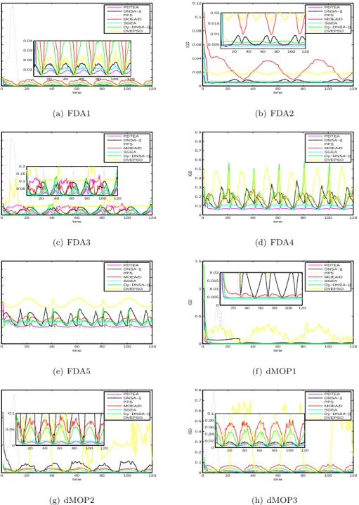
5. Experimental Results and Analysis
In order to compare the effect of change frequency on the compared algo-rithms in dynamic environments, the severity of change was fixed to 10, and the frequency of change was set to 20, 25 and 30, respectively. The statistical
540
results of seven algorithms and the mean and standard deviation values of GD, IGD and HV are shown in Table 1, Table 2 and Table 3, respectively. The best values obtained by the seven algorithms are highlighted in bold face, and the Wilcoxon rank-sum [59] test was carried out to indicate significance between different results at the 0.05 significance level.
545
5.1. Results on FDA and dMOP problems
It can be obtained from Table 1 that PDTEA has the minimum values of GD on the majority of FDA and dMOP test suites whose decision variables are linearly related. The smaller values of GD imply that the algorithm had better convergence than the other algorithms. On the whole, PDTEA significantly
550
shows the best convergence among all the compared algorithms on most test problems. For all the problems, at whatever the frequency of change was set,
PDTEA significantly performed better than DNSGA-II, PPS, Dy-NSGA-II
except FDA2 and dMOP1. However, when compared with SGEA, PDTEA
555
failed to show better competition on FDA2, FDA3 and dMOP1. The reason is that the POS of FDA2 and dMOP1 remain fixed. MOEA/D and SGEA preserve many solutions from the last population, which has considerable convergence merits when addressing those DMOPs with unchanged POS.
As shown in Table 2, PDTEA’s IGD performance metric was the best in
560
most of the test problems except FDA2, FDA3 and dMOP1. Therefore, not only did PDTEA have better distribution than the other methods, but also significantly surpassed others in terms of convergence. For FDA2 and FDA3 test instances, the IGD values of SGEA were the best and those of PDTEA ranked the second, proving that the distribution and convergence of PDTEA
565
were only weaker than SGEA in dynamic changes. As for dMOP1, the values of IGD on MOEA/D were the smallest, which were smaller than SGEA and PDTEA. The conclusion can be made that PDTEA performs moderately on problems like dMOP1.
The HVD values were roughly similar to the IGD values on FDA and dMOP
570
displayed in Table 2 and Table 3. The difference is that the number of HVD values on which PDTEA performed best is one more than that of the IGD values. Specifically, for FDA3, PDTEA significantly outperformed all the other approaches in terms of the HVD metric. In addition, PDTEA ranked the second on problem dMOP1 rather than the third, which can be seen in Table 2. Perhaps
575
the main reasons for the analogous performance are they are comprehensive metrics that measure both distribution and convergence. Obviously, PDTEA is preferable to the other algorithms on most FDA and dMOP problems. However, it is slightly inferior to SGEA on FDA2 and dMOP1 indicating SGEA is also promising as a means to solving DMOPs. It should be mentioned that PDTEA
580
showed significantly competent performance on FDA4 and FDA5 in terms of GD, IGD and HVD values, indicating that PDTEA is the most effective and outstanding methodology for solving problems with three goals.
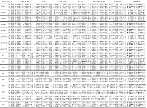
Table 1: Mean and SD of GD indicator obtained by seven algorithms.
Prob (τt, nt) DNSGA-II PPS MOEA/D SGEA Dy-NSGA-II DVEPPSO PDTEA
FDA1(20,10) 1.864e-2(1.627e-3)(25,10) 1.299e-2(3.769e-4)‡‡ 1.415e-1(5.298e-2)9.393e-2(4.835e-2)‡‡1.537e-1(1.577e-2)1.198e-1(9.871e-3)‡‡1.018e-2(1.377e-4)1.328e-2(2.806e-4)‡‡4.100e-2(5.309e-4)7.360e-2(7.220e-4)‡‡7.256e-2(3.417e-2)8.075e-2(7.122e-3)‡‡1.202e-2(7.950e-4)8.455e-3(3.708e-4) (30,10) 1.053e-2(3.025e-4)‡ 7.388e-2(3.935e-2)‡9.629e-2(5.029e-3)‡8.245e-3(1.123e-4)‡2.765e-2(3.690e-4)‡2.332e-2(7.571e-2)‡6.534e-3(2.104e-4) FDA2(20,10) 5.411e-2(3.267e-3)(25,10) 5.617e-2(1.164e-3)‡‡ 1.476e-2(8.575e-4)1.413e-2(5.813e-4)‡‡ 4.264e-3(1.831e-4)4.994e-3(7.572e-4)3.502e-3(8.584e-5)3.586e-3(9.473e-5)1.166e-2(4.926e-5)1.180e-2(1.330e-4)‡‡6.870e-2(1.537e-2)7.104e-2(2.024e-2)‡‡ 8.256e-3(1.592e-4)8.053e-3(2.219e-4)
(30,10) 5.816e-2(1.801e-3)‡ 1.376e-2(5.729e-4)‡ 4.117e-3(1.821e-4)3.457e-3(9.602e-5)1.168e-2(1.448e-4)‡1.677e-2(1.230e-1)‡ 7.937e-3(2.582e-4) FDA3(20,10) 9.314e-2(1.592e-3)(25,10) 9.317e-2(8.440e-4)‡‡ 2.272e-1(8.867e-2)1.893e-1(7.075e-2)‡‡1.481e-1(8.468e-3)1.375e-1(1.344e-2)‡‡5.285e-2(1.294e-3)5.619e-2(1.395e-3)8.351e-2(1.484e-3)1.080e-1(1.410e-3)‡‡9.870e-1(1.537e-2)1.027e-1(3.532e-2)‡‡ 6.570e-2(1.694e-3)6.100e-2(1.129e-3) (30,10) 9.452e-2(9.969e-4)‡ 1.424e-1(8.271e-2)‡1.284e-1(8.314e-3)‡5.225e-2(8.291e-4)7.340e-2(1.911e-3)‡7.415e-2(7.984e-1)‡ 6.033e-2(1.436e-3) FDA4(20,10) 2.716e-1(1.760e-2)(25,10) 2.148e-1(6.485e-3)‡‡ 1.842e-1(6.403e-3)1.616e-1(5.173e-3)‡‡2.635e-1(3.234e-3)1.775e-1(8.682e-3)‡‡8.998e-2(2.275e-3)1.281e-1(9.409e-3)‡‡2.390e-1(5.087e-3)3.161e-1(4.494e-3)‡‡1.925e-1(2.482e-2)1.977e-1(1.300e-2)‡‡6.588e-2(3.115e-3)5.152e-2(2.452e-3)
(30,10) 1.758e-1(5.891e-3)‡ 1.475e-1(4.414e-3)‡1.295e-1(5.197e-3)‡7.018e-2(1.593e-3)‡1.887e-1(1.628e-3)‡1.896e-1(6.469e-2)‡4.047e-2(1.145e-3) FDA5(20,10) 9.726e-1(2.030e-2)(25,10) 9.036e-1(1.108e-2)‡‡ 8.127e-1(7.952e-3)7.953e-1(3.834e-3)‡‡8.611e-1(1.847e-2)7.596e-1(2.250e-2)‡‡7.344e-1(3.012e-3)7.696e-1(4.309e-3)‡‡7.474e-1(8.601e-3)8.095e-1(6.878e-3)‡‡8.629e-1(1.384e-2)9.679e-1(1.282e-2)‡‡6.946e-1(1.691e-3)6.817e-1(1.260e-3) (30,10) 8.565e-1(1.298e-2)‡ 8.125e-1(6.188e-3)‡7.338e-1(1.033e-2)‡7.131e-1(1.657e-3)‡7.009e-1(8.171e-3)‡7.132e-1(3.750e-2)‡6.838e-1(1.710e-3) dMOP1(20,10) 3.921e-2(7.894e-3)(25,10) 2.529e-2(7.177e-3)‡‡ 6.045e-2(1.052e-1)5.223e-2(1.215e-1)‡‡ 7.279e-3(1.386e-3)1.086e-2(5.786e-3)1.712e-3(1.835e-4)2.394e-3(5.232e-4)2.331e-2(2.401e-3)3.708e-2(9.088e-3)‡‡3.261e-2(1.141e-2)3.268e-2(4.673e-1)‡‡ 2.964e-2(3.848e-3)1.582e-2(4.326e-3)
(30,10) 1.968e-2(3.241e-3)‡ 5.365e-2(1.157e-1)‡ 7.203e-3(1.030e-2)1.417e-3(1.137e-4)1.337e-2(1.933e-3)‡2.918e-2(5.267e-2)‡ 1.047e-2(3.073e-3) dMOP2(20,10) 2.098e-1(8.638e-3)(25,10) 1.323e-1(2.636e-3)‡‡ 1.256e-1(5.719e-2)1.776e-1(6.551e-2)‡‡1.105e-1(6.435e-3)1.444e-1(2.056e-2)‡‡1.602e-2(3.434e-4)1.213e-2(3.596e-4)‡9.847e-2(2.689e-3)5.630e-2(1.145e-3)‡‡9.132e-2(5.086e-2)8.128e-2(5.718e-2)‡‡1.133e-2(5.974e-4)1.680e-2(5.605e-4)
(30,10) 8.803e-2(2.438e-3)‡ 9.210e-2(5.865e-2)‡8.814e-2(5.897e-3)‡9.625e-3(1.275e-4)‡3.695e-2(6.275e-4)‡5.519e-2(4.356e-1)‡8.540e-3(3.605e-4) dMOP3(20,10) 1.775e-2(9.973e-4)(25,10) 1.321e-2(3.710e-4)‡‡ 1.229e-1(5.109e-2)1.073e-1(3.057e-2)‡‡1.615e-1(1.980e-2)1.173e-1(1.992e-2)‡‡1.034e-2(2.003e-4)1.333e-2(3.327e-4)‡‡4.123e-2(9.276e-4)7.586e-2(2.004e-3)‡‡5.040e-2(3.146e-2)6.055e-2(1.385e-1)‡‡1.197e-2(5.173e-4)8.623e-3(2.076e-4) (30,10) 1.047e-2(2.192e-4)‡ 6.286e-2(3.212e-2)‡9.716e-2(1.076e-2)‡8.245e-3(1.123e-4)‡2.744e-2(5.346e-4)‡3.421e-2(1.884e-1)‡6.605e-3(2.807e-4) JY1 (20,10) 1.762e+1(8.565e-1)(25,10) 1.671e+1(4.753e-1)‡‡1.692e-1(6.709e-2)1.221e-1(5.465e-2)‡‡1.151e-1(1.058e-2)7.844e-2(2.199e-3)‡‡1.149e-2(2.399e-4)1.559e-2(6.386e-4)‡‡4.405e-2(8.706e-4)8.217e-2(1.634e-3)‡‡2.360e-2(3.931e-2)2.588e-1(4.986e-2)‡‡9.586e-3(4.041e-4)6.274e-3(3.619e-4) (30,10) 1.514e+1(8.146e-1)‡8.030e-2(4.914e-2)‡6.057e-2(6.768e-3)‡9.020e-3(1.383e-4)‡2.742e-2(4.653e-4)‡1.208e-2(2.813e-3)‡4.560e-3(1.964e-4) JY2 (20,10) 4.356e-1(6.730e-2)(25,10) 5.042e-1(4.582e-2)‡‡ 1.918e-1(4.131e-2)1.479e-1(6.333e-2)‡‡1.337e-1(1.732e-2)1.078e-1(7.429e-3)‡‡4.895e-2(3.005e-4)4.922e-2(4.734e-4)6.517e-2(1.196e-3)1.040e-1(2.018e-3)‡‡8.327e-2(7.531e-2)2.499e-1(4.207e-2)‡‡ 5.153e-2(7.873e-4)4.922e-2(2.708e-4)
(30,10) 4.368e-1(9.359e-2)‡ 1.055e-1(3.218e-2)‡9.790e-2(9.117e-3)‡4.846e-2(3.016e-4)†5.602e-2(6.958e-4)‡7.661e-2(3.757e-3)‡4.827e-2(2.962e-4) JY3 (20,10) 3.932e-1(1.442e-1)(25,10) 3.682e-1(1.233e-1)‡‡ 3.810e-1(5.487e-2)3.335e-1(3.841e-2)‡‡2.211e-1(7.559e-3)2.381e-1(3.418e-2)‡‡2.133e-1(8.664e-3)2.018e-1(8.245e-3)‡‡2.455e-1(1.960e-2)2.546e-1(1.934e-2)‡‡1.245e-1(2.544e-1)1.282e-1(3.389e-1)‡‡8.511e-2(5.979e-3)7.582e-2(3.673e-3) (30,10) 3.982e-1(9.665e-2)‡ 3.060e-1(2.381e-2)‡2.096e-1(7.009e-3)‡2.137e-1(8.311e-3)‡2.497e-1(7.664e-3)‡9.193e-2(5.267e-1)‡7.224e-2(3.069e-3) JY4 (20,10) 1.801e+1(5.105e-1)(25,10) 1.915e+1(2.748e-1)‡‡5.227e+0(2.046e-1)5.415e+0(1.527e-1)‡‡4.975e-2(4.604e-3)3.267e-2(2.640e-3)‡‡1.195e+1(3.581e-1)1.000e+1(8.669e-1)‡‡1.035e+1(3.881e-1)1.016e+1(1.427e-1)‡‡8.942e-1(3.024e-2)9.952e-1(3.199e-2)‡‡1.894e-2(6.205e-4)1.498e-2(5.121e-4) (30,10) 1.960e+1(2.436e-1)‡5.560e+0(1.671e-1)‡2.369e-2(1.400e-3)‡1.313e+1(3.972e-1)‡1.129e+1(2.292e-1)‡7.635e-1(3.311e-1)‡1.305e-2(2.644e-4) JY5 (20,10) 1.112e+0(6.984e-2)(25,10) 1.303e+0(1.244e-1)‡‡2.223e-2(2.002e-2)2.021e-2(1.891e-2)‡‡3.474e-3(7.823e-4)2.693e-3(3.153e-4)‡‡1.335e-3(1.282e-4)2.090e-3(6.080e-4)‡2.237e-3(4.041e-4)3.433e-3(6.811e-4)‡‡8.063e-3(4.317e-2)8.866e-3(2.073e-2)‡‡1.827e-3(8.456e-5)1.381e-3(1.031e-4) (30,10) 1.380e+0(1.582e-1)‡1.103e-2(1.082e-2)‡2.402e-3(4.442e-4)‡1.167e-3(9.441e-5)†1.868e-3(1.423e-4)‡2.296e-3(3.308e-3)‡1.133e-3(5.977e-5) JY6 (20,10) 7.082e+0(1.840e-1)(25,10) 5.804e+0(1.103e-1)‡‡1.604e+1(3.532e-1)1.475e+1(2.855e-1)‡‡5.825e+0(3.664e-1)4.250e+0(3.032e-1)‡‡1.259e+0(3.185e-2)1.846e+0(9.442e-2)‡‡6.293e+0(6.657e-2)8.556e+0(1.972e-1)‡‡5.688e+0(3.276e-1)6.781e+0(2.587e-1)‡‡1.013e+0(1.003e-1)4.968e-1(3.689e-2) (30,10) 5.050e+0(1.446e-1)‡1.368e+1(3.494e-1)‡3.221e+0(1.542e-1)‡8.267e-1(6.778e-2)‡4.873e+0(1.158e-1)‡3.587e+0(3.066e-1)‡2.951e-1(4.685e-2) JY7 (20,10) 8.493e+0(9.949e-1)(25,10) 6.372e+0(1.049e+0)‡‡9.174e+1(2.054e+0)7.898e+1(1.483e+1)‡‡3.592e+0(6.285e-1)3.090e+0(4.115e-1)‡‡2.018e+0(3.703e-1)3.022e+0(5.353e-1)‡‡9.530e+0(2.387e-1)1.566e+1(5.778e-1)‡‡2.462e+0(2.941e-1)8.464e+0(4.330e-1)‡‡1.384e+0(1.574e-1)9.891e-1(2.298e-1) (30,10) 4.638e+0(6.230e-1)‡7.163e+1(4.035e+0)‡2.910e+0(4.077e-1)‡1.453e+0(6.021e-1)‡5.771e+0(3.838e-1)‡1.385e+0(2.200e-1)‡7.183e-1(1.633e-1) JY8 (25,10) 1.108e-1(2.387e-2)(20,10) 9.263e-2(4.034e-2)‡‡ 1.417e-2(1.196e-2)1.367e-2(1.108e-2)‡‡8.558e-3(2.091e-4)7.634e-3(3.519e-4)‡‡3.198e-3(2.707e-4)3.611e-3(7.295e-4)7.562e-3(4.957e-4)5.539e-3(3.458e-4) 7.993e-3(4.722e-2)†8.824e-3(1.619e-2)‡‡ 7.574e-3(6.901e-4)6.075e-3(4.148e-4)
(30,10) 8.958e-2(3.374e-2)‡ 7.658e-3(5.931e-3)‡7.408e-3(2.984e-4)‡3.148e-3(1.278e-4)5.334e-3(1.805e-4) 7.043e-3(7.130e-4)‡ 6.282e-3(4.827e-4) JY9 (25,10) 3.178e+1(2.542e+0)(20,10) 3.421e+1(4.725e+0)‡‡6.874e-1(1.983e-1)4.915e-1(1.315e-1)‡‡1.866e-1(1.652e-2)1.311e-1(9.550e-3)‡‡1.503e+0(4.961e-2)8.932e-1(4.751e-2)‡‡1.372e-1(7.311e-3)1.962e-1(2.442e-2)‡‡4.641e-1(1.458e-1)4.899e-1(4.554e-2)‡‡9.162e-2(5.189e-3)5.580e-2(4.308e-3)
(30,10) 3.285e+1(2.760e+0)‡3.102e-1(4.210e-2)‡9.892e-2(8.895e-3)‡5.420e-1(4.423e-2)‡7.669e-2(4.564e-3)‡1.044e-1(3.882e-2)‡3.724e-2(3.756e-3)
‡and†indicate PDTEA performs significantly better than and equivalently to the corresponding
algorithm, respectively.
5.2. Results on JY problems
Compared with FDA and dMOP problems, JY problems [28] are a new
585
benchmark suite with several complex characteristics including a nonmonotonic and time-varying relationship among decision variables. Apart from that, the changing types of some problems vary with time from one to another during the optimization process. It can be obtained from Table 1 that PDTEA significantly performed best over other approaches on most JY problems except JY2, JY5
590
and JY8. As for the JY2 problem, PDTEA only showed less convergence than SGEA but obvious significance than the other five methods. In addition, as changing frequency increased, the superiority of SGEA was not so significant. It is likely that PDTEA would outperform SGEA if the frequency of change were to increase to some certain value. When it comes to JY5, PDTEA almost
595
frequency, the better PDTEA performs. For JY8, whose geometry and the number of mixed segments of the POF vary over time, PDTEA performed better than SGEA, which suggests that the decomposition-based mating selection of PDTEA may have had a negative effect on the convergence.
600
It can be seen from Table 2 that the IGD values of PDTEA were smallest on almost all tested problems except JY3, JY5 and JY8, indicating that PDTEA showed almost best diversity and convergence on almost all of the DMOPs apart from JY3, JY5 and JY8. PDTEA only showed worse performance than SGEA on JY5. Additionally, the HVD values of all the compared algorithms can be
605
found in Table. 3. Obviously, the HVD values of PDTEA only performed worse than the other methods on JY5 and JY8, which shows that the PDTEA’s com-prehensive performance in terms of diversity and convergence was only worse when solving problems like JY5 and JY8. All algorithms’ values of HVD on JY5 were the same as those of IGD. It should be noted that PDTEA performed
610
less effectively on JY8, since it only outperformed DNSGA-II, and it performed equally to PPS. However, it also showed worse performance when compared with SGEA. To conclude, the diversity and convergence of PDTEA is worse than that of SGEA on JY5 and JY8. The reason might be that both JY5 and JY8 have the fixed POS, suggesting that PDTEA has less competent
perfor-615
mance when solving DMOPs with an unchanged POS. Additionally, PDTEA demonstrated more significant effectiveness and superiority than most existing DMOEAs when addressing problems with considerable complicated geometry and rather sophisticated characteristics.
5.3. Results onF DA5iso,F DA5dec,dM OP2iso anddM OP2dec 620
The flat regions and a deceptive POF were proposed by Huband et al.[60]
and Helbiget al. [55][54] introduced some dynamic problems with new dynamic
features. We selectedF DA5iso,F DA5dec,dM OP2isoand dM OP2decto
com-pare the algorithms with (τt, nt) = (25, 10) and obtained GD, IGD and HVD
metric values in Table 4. The Wilcoxon signed-rank test [59] was carried out at
625
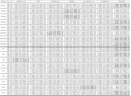
Table 2: Mean and SD of IGD indicator obtained by seven algorithms.
Prob (τt, nt) DNSGA-II PPS MOEA/D SGEA Dy-NSGA-II DVEPSO PDTEA
FDA1(20,10) 2.022e-2(1.976e-3)(25,10) 1.421e-2(3.613e-4)‡‡9.571e-2(3.441e-2)6.604e-2(3.547e-2)‡‡8.544e-2(9.330e-4)6.438e-2(1.213e-3)‡‡1.330e-2(1.366e-3)1.819e-2(1.620e-3)‡‡4.610e-2(4.380e-3)7.570e-2(5.666e-3)‡‡3.632e-2(2.321e-1)4.829e-2(5.155e-2)‡‡1.332e-2(6.584e-4)1.018e-2(3.993e-4) (30,10) 1.205e-2(4.914e-4)‡5.370e-2(2.807e-2)‡5.292e-2(1.494e-3)‡1.087e-2(1.171e-3)‡2.937e-2(6.704e-4)‡1.305e-2(6.150e-2)‡8.522e-3(5.577e-4) FDA2(20,10) 6.706e-3(2.176e-4)(25,10) 6.501e-3(6.459e-5)‡‡7.825e-3(5.325e-4)6.955e-3(2.784e-4)‡‡2.753e-2(2.357e-3)2.946e-2(5.005e-3)‡‡5.122e-3(1.072e-3)4.974e-3(7.323e-4)6.332e-3(1.560e-4)6.543e-3(1.878e-4)‡‡3.277e-2(4.400e-3)3.485e-2(4.802e-3)‡‡5.982e-3(4.199e-4)5.980e-3(1.518e-3)
(30,10) 6.603e-3(8.957e-5)‡6.614e-3(2.717e-4)‡2.643e-2(3.046e-3)‡4.839e-3(5.128e-4)6.756e-3(9.676e-4)‡1.974e-2(1.816e-3)‡5.973e-3(9.855e-4) FDA3
(20,10) 5.210e-2(3.113e-3)‡1.528e-1(7.604e-2)‡6.140e-2(2.408e-3)‡2.959e-2(2.174e-3)7.132e-2(4.040e-3)‡3.918e-1(3.327e-2)‡5.300e-2(4.052e-3) (25,10) 5.290e-2(7.743e-3)‡1.164e-1(6.148e-2)‡5.257e-2(5.005e-3)†2.369e-2(2.295e-3)5.149e-2(3.292e-3)†3.720e-1(6.858e-2)‡5.292e-2(3.894e-3) (30,10) 5.065e-2(2.640e-3)‡7.363e-2(7.362e-2)‡4.360e-2(1.692e-3)‡2.134e-2(1.366e-3)3.752e-1(5.124e-3) 1.346e-1(8.375e-1)‡5.132e-2(3.434e-3) FDA4(20,10) 2.112e-1(1.108e-2)(25,10) 1.813e-1(2.338e-3)‡‡1.473e-1(3.328e-3)1.330e-1(2.631e-3)‡‡2.773e-1(5.374e-3)2.091e-1(5.342e-3)‡‡1.071e-1(2.072e-3)1.379e-1(6.425e-3)‡‡2.219e-1(4.870e-3)2.764e-1(2.216e-3)‡‡1.038e-1(1.866e-2)1.089e-1(6.663e-3)‡‡7.660e-2(8.632e-4)7.122e-2(6.186e-4)
(30,10) 1.595e-1(3.965e-3)‡1.251e-1(2.425e-3)‡1.699e-1(2.862e-3)‡9.273e-2(1.382e-3)‡1.850e-1(1.533e-3)‡9.585e-2(4.792e-2)‡6.832e-2(5.677e-4) FDA5(20,10) 8.349e-1(8.508e-3)(25,10) 8.049e-1(7.269e-3)‡‡7.660e-1(6.588e-3)7.491e-1(5.610e-3)‡‡8.848e-1(8.084e-3)8.181e-1(3.189e-3)‡‡7.212e-1(2.172e-3)7.492e-1(3.612e-3)‡‡7.643e-1(6.382e-3)8.130e-1(5.386e-3)‡‡1.162e+0(1.359e-2)1.197e+0(5.857e-3)‡‡6.785e-1(6.646e-4)6.730e-1(6.550e-4) (30,10) 7.823e-1(5.725e-3)‡7.659e-1(5.297e-3)‡7.661e-1(2.102e-3)‡7.042e-1(1.473e-3)‡7.280e-1(6.642e-3)‡1.064e+0(4.287e-2)‡6.695e-1(7.259e-4) dMOP1(20,10) 2.210e-1(3.168e-1)(25,10) 2.647e-2(7.036e-3)‡‡5.467e-2(1.023e-1)5.096e-2(1.106e-1)‡‡1.144e-2(6.079e-4)9.018e-3(7.697e-4)1.035e-2(1.980e-3)1.371e-2(3.039e-3)†‡2.987e-2(3.784e-3)4.112e-2(8.497e-3)‡‡1.891e-1(8.319e-1)1.966e-1(3.453e-1)‡‡2.406e-2(2.293e-3)1.601e-2(3.623e-3)
(30,10) 3.674e-2(4.653e-2)‡5.448e-2(1.100e-1)‡7.980e-3(2.465e-4)9.112e-3(1.514e-3) 2.346e-2(1.926e-3)‡6.292e-2(4.614e-1)‡1.290e-2(3.270e-3) dMOP2(20,10) 1.989e-1(1.225e-2)(25,10) 1.298e-1(8.245e-3)‡‡1.822e-1(8.113e-2)1.271e-1(7.074e-2)‡‡8.473e-2(2.104e-3)6.663e-2(1.200e-3)‡‡1.508e-2(1.760e-3)2.102e-2(2.355e-3)‡‡5.563e-2(4.724e-3)9.864e-2(5.531e-3)‡‡8.926e-1(7.577e-2)9.063e-1(3.020e-2)‡‡1.741e-2(5.740e-4)1.264e-2(8.063e-4)
(30,10) 1.128e-1(3.101e-2)‡8.432e-2(6.315e-2)‡5.459e-2(1.006e-3)‡1.276e-2(1.156e-3)‡3.620e-2(2.281e-3)‡5.131e-1(5.181e-1)‡9.958e-3(3.647e-4) dMOP3(20,10) 2.009e-2(1.623e-3)(25,10) 1.456e-2(4.768e-4)‡‡8.324e-2(3.417e-2)7.419e-2(2.220e-2)‡‡8.441e-2(1.740e-3)6.444e-2(1.629e-3)‡‡1.304e-2(1.645e-3)1.715e-2(1.032e-3)‡‡4.477e-2(3.142e-3)7.960e-2(4.563e-3)‡‡8.104e-2(7.943e-2)8.216e-2(4.080e-2)‡‡1.374e-2(7.663e-4)1.047e-2(4.878e-4) (30,10) 1.227e-2(8.990e-4)‡4.464e-2(2.205e-2)‡5.267e-2(1.498e-3)‡1.087e-2(1.171e-3)‡2.957e-2(1.437e-3)‡6.462e-2(1.661e-1)‡8.925e-3(7.248e-4) JY1 (20,10) 2.523e-1(3.422e-2)(25,10) 1.415e-1(1.427e-2)‡‡1.032e-1(4.086e-2)7.835e-2(3.517e-2)‡‡7.128e-2(1.643e-3)5.535e-2(7.810e-4)‡‡2.255e-2(1.231e-3)2.946e-2(9.175e-4)‡‡4.602e-2(5.334e-4)7.284e-2(1.041e-3)‡‡8.198e-2(3.088e-2)9.763e-2(1.396e-2)‡‡1.261e-2(4.350e-4)9.635e-3(2.646e-4) (30,10) 9.371e-2(1.336e-2)‡5.365e-2(3.063e-2)‡4.644e-2(6.062e-4)‡1.799e-2(7.981e-4)‡3.299e-2(7.575e-4)‡7.110e-2(3.324e-3)‡7.950e-3(1.965e-4) JY2 (20,10) 5.832e-2(5.740e-4)(25,10) 5.473e-2(4.618e-4)‡‡1.361e-1(2.756e-2)1.113e-1(3.998e-2)‡‡8.769e-2(1.643e-3)7.457e-2(6.048e-4)‡‡5.431e-2(3.039e-4)5.810e-2(7.660e-4)‡‡6.710e-2(4.497e-4)8.971e-2(1.195e-3)‡‡9.021e-2(3.740e-2)1.786e-1(1.377e-2)‡‡5.199e-2(3.655e-4)5.024e-2(1.327e-4) (30,10) 5.289e-2(3.052e-4)‡8.574e-2(2.066e-2)‡5.136e-2(4.026e-3)‡5.294e-2(5.343e-4)‡5.998e-2(3.502e-4)‡8.835e-2(4.011e-3)‡4.963e-2(1.268e-4) JY3 (20,10)(25,10)2.736e-1(2.811e-3)2.742e-1(1.318e-2)3.477e-1(1.993e-2)3.321e-1(1.473e-2)‡‡3.227e-1(4.731e-3)3.334e-1(2.141e-2)†‡3.317e-1(5.784e-3)3.329e-1(1.212e-2)‡‡3.164e-1(2.027e-3)3.242e-1(8.134e-3)‡†2.901e+0(1.293e-1)3.103e+0(4.162e-2)‡‡3.152e-1(3.821e-3)3.089e-1(2.988e-3)
(30,10)2.685e-1(1.281e-3)3.219e-1(7.532e-3)‡3.136e-1(4.026e-3)†3.319e-1(8.720e-3)‡3.129e-1(1.710e-3)†1.350e+0(7.902e-1)‡3.070e-1(2.158e-3) JY4 (20,10) 3.880e-1(2.407e-2)(25,10) 3.201e-1(1.186e-2)‡‡6.734e-1(2.965e-2)5.667e-1(3.582e-2)‡‡7.875e-1(1.599e-3)6.082e-1(1.062e-3)‡‡1.354e+0(7.506e-2)1.423e+0(1.375e-1)‡‡1.231e+0(2.916e-2)1.414e+0(6.990e-2)‡‡7.673e-1(1.559e-2)8.283e-1(1.813e-2)‡‡2.216e-2(6.820e-4)1.959e-2(2.429e-4)
(30,10) 3.003e-1(8.792e-3)‡4.879e-1(3.009e-2)‡4.993e-1(1.310e-3)‡1.346e+0(7.247e-2)‡1.105e+0(5.621e-3)‡7.082e-1(5.987e-2)‡1.858e-2(1.823e-4) JY5 (20,10) 3.002e-2(2.614e-4)(25,10) 3.006e-2(3.037e-4)‡‡1.726e-2(1.282e-2)1.611e-2(1.217e-2)‡‡1.031e-2(3.394e-4)9.420e-3(2.687e-4)‡‡4.345e-3(4.604e-5)4.703e-3(1.805e-4)5.615e-3(1.348e-4)6.002e-3(2.497e-4)‡‡3.927e-2(1.988e-2)4.252e-2(6.329e-3)‡‡5.600e-3(9.765e-5)5.454e-3(1.298e-4)
(30,10) 3.000e-2(2.518e-4)‡1.069e-2(7.531e-3)‡8.560e-3(4.505e-4)‡4.260e-3(3.994e-5)5.474e-3(3.634e-5)‡2.143e-2(2.059e-3)‡5.371e-3(1.736e-4) JY6 (25,10) 3.079e+0(1.148e-1)(20,10) 3.674e+0(1.557e-1)‡‡7.642e+0(1.858e-1)7.088e+0(1.697e-1)‡‡3.711e+0(1.884e-1)2.405e+0(1.866e-1)‡‡1.027e+0(3.530e-2)7.111e-1(1.492e-2)‡‡3.297e+0(4.110e-2)4.480e+0(1.265e-1)‡‡6.445e+0(7.806e-2)6.771e+0(7.680e-2)‡‡3.135e-1(4.329e-2)2.507e-1(1.768e-2)
(30,10) 2.825e+0(1.197e-1)‡6.598e+0(1.615e-1)‡1.807e+0(1.081e-1)‡5.033e-1(2.724e-2)‡2.568e+0(6.526e-2)‡2.996e+0(2.261e-1)‡1.617e-1(2.109e-2) JY7 (20,10) 3.506e+0(5.065e-1)(25,10) 2.745e+0(6.109e-1)‡‡2.517e+1(5.143e+0)2.932e+1(9.855e-1)‡‡1.822e+0(4.354e-1)1.674e+0(2.402e-1)‡‡1.145e+0(1.955e-1)1.625e+0(2.611e-1)‡‡3.846e+0(1.546e-1)6.164e+0(1.835e-1)‡‡5.636e+0(7.069e-2)5.789e+0(1.205e-1)‡‡7.771e-1(1.084e-1)5.700e-1(1.426e-1) (30,10) 2.035e+0(3.533e-1)‡2.242e+1(2.122e+0)‡1.633e+0(3.053e-1)‡9.161e-1(3.725e-1)‡2.296e+0(2.833e-1)‡8.886e-1(1.888e-1)‡4.539e-1(1.098e-1) JY8 (20,10) 7.302e-1(3.018e-2)(25,10) 1.845e-1(2.101e-2)‡‡1.340e-2(6.890e-3)1.310e-2(6.314e-3)‡‡2.655e-2(1.055e-3)2.395e-2(1.112e-3)‡‡1.640e-2(2.055e-3)1.765e-2(2.714e-3)‡‡8.470e-3(2.188e-4)9.249e-3(2.396e-4)3.615e-2(1.343e-2)4.010e-2(3.687e-3)‡‡1.107e-2(6.598e-4)1.068e-2(7.110e-4)
(30,10) 9.661e-2(3.540e-2)‡9.744e-3(3.355e-3)†2.165e-2(6.311e-4)‡1.482e-2(1.163e-3)‡8.738e-3(2.785e-4)1.595e-2(6.655e-4)‡9.747e-3(5.968e-4) JY9 (25,10) 2.710e-1(4.191e-2)(20,10) 5.278e-1(1.465e-1)‡‡3.798e-1(1.192e-1)2.786e-1(7.439e-2)‡‡1.207e-1(9.859e-3)8.756e-2(3.907e-3)‡‡1.061e+0(3.599e-2)6.365e-1(2.567e-2)‡‡9.810e-2(6.914e-3)1.359e-1(1.624e-2)‡‡2.063e-1(2.769e-2)2.192e-1(1.212e-2)‡‡6.820e-2(3.114e-3)4.255e-2(3.721e-3)
(30,10) 1.898e-1(3.239e-2)‡1.783e-1(2.386e-2)‡6.427e-2(2.989e-3)‡3.881e-1(3.593e-2)‡5.865e-2(2.314e-3)‡9.646e-2(3.540e-2)‡3.024e-2(3.049e-3)
‡and†indicate PDTEA performs significantly better than and equivalently to the corresponding algorithm,
respectively.
DPTEA and the other algorithms.
It can be observed from Table 4 that most algorithms obtained worse metric values on the problems with dynamic features, implying the problem is chal-lenging for DMOEAs. PDTEA can deal with a majority of problems except
630
dM OP2iso according to three metrics. The result of SGEA ondM OP2iso
in-dicates that SGEA is a top performer on the problem. This is because SGEA uses the steady-state population update to significantly improve performance.
ForF DA5dec with a deceptive POF, PDTEA shows superior performance by
IGD and HVD values, while the GD value indicates SGEA has a good
conver-635
gence performance. The reason is that PDTEA uses the exploration strategy to improve the population’s diversity. Hence, the exploration strategy is helpful to deal with the deceptive POF. Nevertheless, the steady-state update in SGEA may cause the loss of diversity.