Toward the Online Visualisation of Algorithm
Performance for Parameter Selection
David J. Walker1and Matthew J. Craven2 1
University of Exeter, United Kingdom ([email protected])
2
University of Plymouth, United Kingdom ([email protected])
Abstract. A visualisation method is presented that is intended to as-sist evolutionary algorithm users with the parametrisation of their algo-rithms. The visualisation method presents the convergence and diversity properties such that different parametrisations can be easily compared, and poor performing parameter sets can be easily identified and dis-carded. The efficacy of the visualisation is presented using a set of bench-mark optimisation problems from the literature, as well as a benchbench-mark water distribution network design problem. Results show that it is pos-sible to observe the different performance caused by different parametri-sations. Future work discusses the potential of this visualisation within an online tool that will enable a user to discard poor parametrisations as they execute to free up resources for better ones.
Keywords: Visualisation, Multi-objective, Optimisation, Water Distri-bution Network Design.
1
Introduction
Visualisation remains an open problem within evolutionary computation (EC). Recently, considerable effort has been expended in investigating methods for visualising sets of solutions, with the aim of presenting the final set of generated solutions to a decision maker so that one can be selected for implementation. The visualisation of algorithm performance lags somewhat behind. Such visualisation is an important avenue of research, as useful visualisations of algorithm operation can help to reveal the inner workings of an evolutionary algorithm (EA), which to a non-expert are a black box. By exposing the operation of an EA to a non-expert user, the uptake of evolutionary computation by industry will be increased.
This paper presents a new visualisation that is intended to assist an algo-rithm user when parametrising their algoalgo-rithms. All varieties of EA require a range of parameters to be set. Most, including genetic algorithms (GAs), dif-ferential evolution (DE) and particle swarm optimisation (PSO) are extremely sensitive to their parameters being set correctly, with a poor set of parameters resulting in a poor set of solutions. The EC literature contains a range of ways of characterising performance; in this work, multi-objective problems are consid-ered, and algorithm performance is characterised in terms of convergence to the true Pareto front and population diversity. Both of these aspects are revealed
through the proposed visualisation, and a “good” parametrisation requires both good convergence and population diversity.
The visualisation is demonstrated on well-known continuous test problems from the literature (the DTLZ problem suite [7]). Problems are selected that will demonstrate the algorithm’s performance on a range of problem characteristics. As well as these problems, an industrial benchmark problem is demonstrated – the water distribution network design problem. This is a combinatoric problem, and represents a class of problem that are commonly optimised using EAs. The paper is structured as follows: a brief survey of relevant visualisation approaches is presented in Section 2 before the proposed visualisation is introduced in Sec-tion 3. The experimental framework is discussed and the visualisaSec-tion method demonstrated in Section 4, before its results are discussed in Section 5. The final section serves as a conclusion to the paper, as well as containing as discussion of future work.
2
Background
2.1 Multi-objective Optimisation
This paper is concerned with continuous and discrete multi-objective optimisa-tion problems. In both cases, consider a soluoptimisa-tionx, whereinxpis one ofP deci-sion variables. Solution quality is determined with a set ofM objective functions
fm, forming an objective vectory:
y= (f1(x), . . . , fM(x)). (1) Relative solution quality is assessed using dominance, such that given two so-lutions xi is superior toxj if it dominates xj. This is the case if it is no worse
than xj on all objectives and better on at least one (assuming a minimisation
problem, without loss of generality):
yi≺yj⇐⇒ ∀m(yim≤yjm)∧ ∃m(yim< yjm). (2)
If neither of two solutions dominate the other then they are called mutually non-dominating. If a solution has no dominating solutions, it is said to be non-dominated. The optimal set of solutions are called the Pareto set, which map to the Pareto front in objective space. This is the mutually non-dominated set of non-dominated feasible solutions, and represents the best possible trade-off between the problem objectives. In order to produce a suitable estimate of the Pareto front, the job of a multi-objective EA (MOEA) is to converge to a point close to the Pareto front, and cover the front’s full extent.
2.2 Visualisation of Evolution
Of the visualisation work within EC, a considerable amount is focused on dis-playing populations of solutions (e.g., [3, 15]). In particular, many-objective opti-misation (wherein problems comprise four or more objectives) pose a particular
challenge for visualisation [15], as human decision makers can only comprehend three or fewer spatial dimensions. Many-objective problems are not considered herein, however current ongoing work is considering how they can be incorpo-rated into the proposed framework.
Fewer publications consider visualising the process of evolution itself. An example that is directly relevant to this work is proposed in [5], which uses a visualisation method to assess the stability of parameters for an EA used to solve a single-objective cryptology problem. They define metrics over the parameter space3and perturb parameters to show the effect of moving them around within a small neighbourhood. One of the first examples of visualisation work within the EC field was [13], which proposed a set of standard tools for visualising solutions, populations, and algorithm characteristics such as convergence. A similar system was proposed by [12], which allowed a user to view the propogation of genetic material throughout the execution of an EA (they optimised the 0/1 Knapsack problem). Elsewhere, an example of a tool that seeks to visualise the evolution process is GAVEL [10], which presents maps of populations of solutions in terms of the genetic operators used to generate them. Other aspects of the tool show the rate at which solutions are generated, as well as fitness information. A visu-alisation developed for water distribution network (WDN) design was proposed by [11] in which a visualisation of a single solution (a single WDN) is coloured according to the frequency that each decision variable (an individual pipe diam-eter) within the solution is perturbed. Within the realm of genetic programming there have been various examples of visualising the ancestry of solutions (e.g., [4]).
3
Visualising Stability Within Multi-objective EAs
The method proposed herein visualises the stability of an algorithm’s parameters by showing how important properties of a MOEA (such as convergence to the Pareto front and diversity within the population) change over time for given parametrisations of algorithms.
Fig. 1 shows a schematic describing the construction of the visualisation. The plot itself is circular, and is designed to contain information about multiple executions of an EA. Each point within the visualisation represents a single solution within an algorithm’s population for a single generation, and has three degrees of freedom: its angle from the origin, distance from the centre of the plot, and its colour; each of these is used to convey an aspect of algorithm performance. The choice of characteristic these variables are used to show is up to the user to decide. Two important aspects of the execution of a MOEA are convergence, to ensure that the algorithm generates solutions that are close to the true Pareto front, and diversity, to ensure that the search population is properly explored. This work utilises two well-known measures from the evolutionary computation
3
Herein the termparameteris used to refer to algorithm parameters;decision variable
θ r
O
Fig. 1: A schematic showing the placement of a solution within the visualisation.
literature to illustrate both characteristics across a set of algorithms optimising benchmark test problems.
To show convergence, the hypervolume indicator [8] is employed. This pro-vides a measure of dominated space between the current search population and a reference point; in this work, the hypervolume of individual solutions is con-sidered. A reference point is computed by taking the maximum value for each objective seen at any point in the optimisation process. As the population con-verges, the distance from this reference point increases. Hypervolume is used to determine the angle θ by multiplying the hypervolume value (lying between 0 and 1 as a proportion of the space that could be dominated) by 2π. At the begin-ning of an optimisation run, when working with randomly generated solutions, points are typically scattered across the extent of the circle. As more optimal solutions are generated, and the algorithm converges towards the true Pareto front, this angle decreases and the population tend to be clustered around the origin (shown by a dotted line and the label “O” in Fig. 1).
Diversity is evaluated using the crowding distance. Crowding distance pro-vides a measure of the proximity of the nearest solution in each objective, and is well-known for its use in the selection operator of NSGA-II [6]. It is important to note the flexibility of the proposed method. In this work, hypervolume and crowding distance have been used as well-known measures of convergence and diversity that do not require a priori knowledge about the true Pareto front (which is known for the continuous test problems tested later, but not for the industrial benchmark problem also demonstrated). These indicators can be eas-ily substituted for any measure required – for example, an indicator of decision space diversity, or measures indicating (for example) velocities within a particle swarm optimiser. These are aspects of ongoing work, which are not discussed further in this paper.
4
Experimental Setup
In order to demonstrate the potential of the proposed method, continuous test problems from the multi-objective literature are considered, before an industrial benchmark is evaluated.
4.1 Continuous Test Problems
Three benchmark multi-objective problems from the literature are optimised with three variants of a basic MOEA, and the various algorithm performances are visualised. The test problems employed are a 2-objective DTLZ1 and a 3-objective DTLZ2 [7], both of which have different problem characteristics. Both are real-valued, with legal parameters in the range (0,1). To facilitate an easier analysis of the visualisations, the MOEA works with a population size of 10. DTLZ1 is known to be a harder problem than DTLZ2; as such, the optimiser executes for 5,000 generations, while DTLZ2 is optimised for 500 generations.
Three algorithms are selected for their different optimisation behaviours; all three variants follow the same basic arrangement. The algorithm begins by initialising a random search population, which is evaluated under the problem objective functions. An elite archive, in which the current approximation to the Pareto front will be stored, is initialised. The archive is passive, in that it does not participate in the evolutionary process. At each generation, a child population is generated by applying crossover and mutation operators, and is evaluated under the objectives. The archive is updated, so that any newly dominated solutions are removed, and any members of the child population that are not dominated by members of the archive are added to it. Finally, elitist selection is applied to the combined parent and child populations to select the parent population for the next generation. The specific operators used to obtain specific optimisation behaviours are now discussed.
In the first EA, single-point crossover is used to combine two candidate parent solutions chosen at random. A child solution is created by joining the decision variables prior to the crossover point on one of the parents with the decision variables following the crossover point on the other. The child is then mutated using an additive Gaussian mutation, and evaluated. To demonstrate different parametrisations of the algorithm, the standard deviation of the Gaussian dis-tribution from which the additive mutation is drawn is chosen randomly in the range (0,1). The selection operator performs non-dominated sorting on the com-bined parent and child populations. As solutions are added to the new parent population, if the current non-dominated front contains more solutions than are needed to fill the population then the number required are selected from that front at random. This algorithm provides good convergence to the Pareto front, and is able to cover its full extent, so providing an example of an optimiser with good performance.
The second EA operates largely in the same way as the first. It generates so-lutions using the crossover and mutation operators described above, and uses the
archive in the same way. The difference is in the choice of selection operator; av-erage rank[2] is used to determined which solutions are carried forward into the next generation. Average rank is a method proposed to deal with many-objective optimisation problems, where non-dominated sorting is unable to provide suffi-cient selection pressure to properly optimise [9]. It is formalised as follows:
¯ ri= 1 M M X m=1 rim, (3)
where rim is the rank of thei-th solution when ranked according to the m-th objective. Having ranked the population, the topNsolutions from the combined parent and child populations are retained. On its own, average rank is able to provide extremely good convergence to the Pareto front, but this is at the expense of the diversity. The resulting approximation to the Pareto front is clustered around the extremes of the front, where the lowest objective values, and therefore the best ranks, are to be found. This is used herein as an example of an optimiser suffering from premature convergence.
The final algorithm is a random search of the feasible space, and is used to highlight an example of poor convergence. Rather than retaining the fittest solutions, a population ofN solutions is chosen uniformly at random from the 2N-member combination of the parent and child populations.
4.2 Water Distribution Network Design
In addition to the continuous test problems demonstrated in the previous sec-tion, the algorithm is used to optimise a benchmark water distribution network (WDN) design problem from the field of hydroinformatics. This problem is dis-crete, requiring the identification of a set of pipe diameters that will form the optimal WDN. The problem is multi-objective, with a candidate network eval-uated both in terms of its cost and its hydraulic properties.
The New York Tunnels problem [14] comprises 21 nodes connected by 20 pipes. The correct diameter for each pipe must be identified, from one of 16 possibilities. Hence, the feasible search space is of size 2016 ≈6.55×10²⁰. The problem objectives are formulated as follows:
f1= K X k=1 1.1d1k.24×lk , (4) f2= N X n=1 ˆ hn−hn>0. (5)
The diameter of the k-th pipe is given by dk, while lk represents that pipe’s length. Thehead deficitfor nodenis specified byhn, and ˆhn is the target head deficit for that node.
Whereas the continuous problems are optimised with fifty parametrisations of an additive Gaussian mutation, this problem must be optimised with combi-natoric perturbations. The crossover portion of the MOEA is retained, and the mutation operator is swapped with one of five different heuristics:
– Change by one size:a randomly chosen pipe’s diameter is replaced with the next largest or smallest available diameter (also known as creep muta-tion).
– Shuffle: a randomly selected block of diameters is randomly reordered. – Ruin & recreate:the solution is replaced with an entirely new chromosome. – Change pipe: a randomly chosen pipe’s diameter is replaced with a
ran-domly chosen available pipe.
– Swap: two randomly chosen pipe diameters are swapped.
As before, the algorithm operates with a population of 10 solutions and runs for 5,000 generations.
5
Results
5.1 DTLZ2
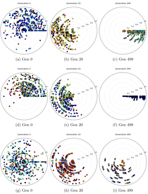
The first set of visualisation, shown in Fig. 2, demonstrates the optimisation of DTLZ2. The figure presents a grid of nine visualisations. Each row shows a different algorithm’s optimisation progress: the top row shows the Pareto sorting-based algorithm; the second row is average rank, and the bottom row shows the random selection strategy. In each case, the left-hand column shows the popula-tion after selecpopula-tion in the first generapopula-tion; the middle column shows generapopula-tion 20 and the right-hand column shows the final search population. Each visualisation shows the ten solutions comprising a population for each of the fifty algorithm parametrisations.
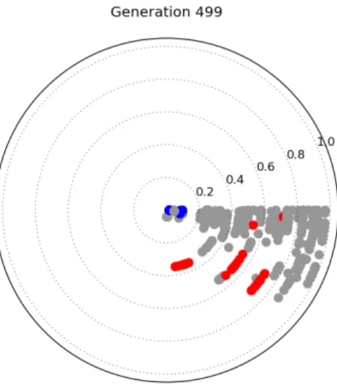
The ideal situation is shown by the top row, presenting results for the Pareto sorting approach. As can be seen, the solutions have progressed around the arc of the visualisation, and are clustered around the zero angle line. This indicates that most of the populations have converged to a good approximation of the Pareto front, as their hypervolume is close to the optimal observed value. Some of the populations have not quite converged. The final population is repeated in Fig. 3, which shows this in more detail. Six of the parametrisations have been highlighted – those shown in blue have converged, and those shown in red have not. Recalling that the distance from the centre of the visualisation represents the standard deviation of the additive Gaussian mutation applied to the chosen parameter, this is intuitively correct. Small Gaussian mutations are known to provide better convergence than larger ones, which cause behaviour closer to a random walk through the space. Returning to Fig. 2, the diversity within the population is also good. As can be seen, the colours of the points representing solutions are a mixture of light blues and oranges. This indicates a mixture of solutions with medium crowding distances, and suggests that the algorithms
(a) Gen 0 (b) Gen 20 (c) Gen 499
(d) Gen 0 (e) Gen 20 (f) Gen 499
(g) Gen 0 (h) Gen 20 (i) Gen 499
Fig. 2: Visualisations of DTLZ2. The top row shows the populations generated by using the basic GA; the middle row shows corresponding results for the average rank optimiser, and the bottom row for the random solution generation algo-rithm. Colour indicates crowding distance – a low crowding distance is shown in blue, high distances are in red.
Fig. 3: The final set of populations for the algorithm using Pareto sorting to optimise DTLZ2. The blue group show better convergence than the red group.
have not suffered from a loss of diversity (which would be shown by exclusively small crowding distances – blue solutions, in the visualisations).
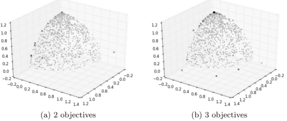
The bottom two rows show less satisfactory behaviour of the optimisers. The middle row shows a set of results for an optimiser using average rank. At first glance, the optimiser has performed well; the solutions are very well converged to the true Pareto front. In fact, they are closer to the optimal set of solutions than those generated using Pareto sorting. Unfortunately, this convergence is premature, and is at the expense of the diversity within the population. As can be seen, the solutions are generally dark blue, indicating a low crowding distance. The effect of this can be seen in the example Pareto front shown in Fig. 4, which shows two final estimated Pareto fronts from the last generation of the average rank optimiser. In both cases, the solutions (shown with black crosses) are generally clustered around the edges and corners of the true Pareto front (samples of which are shown with grey dots). Though these solutions are very close to the front (with a few exceptions, which are too close to minimising one of the objectives that they are extremely difficult to dominate) they do not properly cover the front. A large proportion of the true Pareto front is unexplored by the optimiser, and the resulting solution set does not properly describe the trade-off between objectives. The final row has the opposite problem: optimised using a random selection operator, there is very little selection pressure to drive the population to the Pareto front. As a result, the populations do not converge, as shown by the large spread of solutions that have not reached the zero angle line. The populations have, however, retained their diversity. As was the case with the Pareto sorting example, solutions are coloured between blue and orange.
(a) 2 objectives (b) 3 objectives
Fig. 4: Exemplar Pareto front approximations for DTLZ2 obtained using average rank selection. Black crosses show the generated solutions; grey dots are samples from the true Pareto front. The optimiser has clearly preferred the corners of the front, with some poor solutions remaining in the archive from early generations.
5.2 DTLZ1
Fig. 5 presents two snapshots from the execution of DTLZ1 using the Pareto sorting optimiser (generations 33 and 96). As can be seen, by this early stage in the optimisation process the algorithm has already made substantial progress in converging toward the true Pareto front – the solutions are all in the bottom section of the visualisation. What is interesting in these visualisations is that it is possible to observe the algorithm dealing with the deceptive fronts present in the test problem. These are locally optimal regions of the search space on which the algorithm becomes stuck, and as can be seen this is occurring during these two generations. Whereas for DTLZ2, smaller mutations were causing more rapid convergence than larger ones, here, the opposite is true. Larger mutation values are causing those populations to converge faster than their slower counterparts, which are struggling to generate mutations strong enough to escape the deceptive fronts on which they have become trapped. Though they will eventually escape, it will take longer with smaller mutations. That said, as the populations reach the true Pareto front, smaller mutations will induce the desired exploitative behaviour that will cover the entire front.
5.3 Water Distribution Network Design
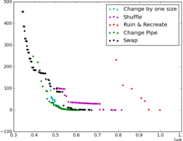
Figs. 6 and 7 present the results for the WDN design problem. Fig. 7 shows the different mutation heuristics used to solve the problem, each of which is shown on its own ring within the visualisation. The left-hand plot shows the initial generation, with a random spread of solutions in the top portion of the visual-isation. The second plot shows generation 20, and the populations are moving
(a) Gen 33 (b) Gen 96
Fig. 5: Two snapshots of the Pareto sorting MOEA optimising DTLZ1. The left-hand visualisation shows the population during generation 33, while the right-hand shows generation 96. Those optimisers with larger standard deviations are advancing faster than those generating smaller mutations, as the optimiser is temporarily stuck on deceptive fronts. This can be seen by the outer cluster of solutions being further around the circle than the inner cluster, in both cases. Eventually, all populations converge over time to the true front. Again, colour indicates diversity.
Fig. 6: The estimated Pareto fronts generated by the optimisers for the New York Tunnels problem.
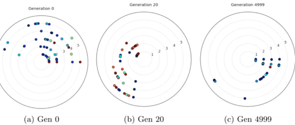
(a) Gen 0 (b) Gen 20 (c) Gen 4999
Fig. 7: Visualisations of algorithm performance. Each ring represents a different perturbation heuristic. 1: change by one size; 2: change pipe; 3: ruin and recre-ate; 4: shuffle; 5: swap. Position indicates convergence while diversity is shown according to the solution colour.
into the lower portion of the visualisation, indicating that they are starting to converge. By the final plot, three of the five heuristics have mostly converged. These include the change by one size heuristic and the change pipe heuristic, which are known to work well on such problems [16]. Neither the ruin and recre-ate heuristic or the swap heuristic have converged. This is intuitively correct, as the ruin and recreate heuristic does not learn from one generation to the next, and the swap heuristic is incapable of introducing novel genetic material. This is confirmed by the Pareto front approximation generated in each case, and shown in Fig. 6 (neither front has converged toward the knee identified by the other heuristics). That said, from observing the colouring in Fig. 7, the swap heuristic has the most diverse population. The effect of this is to generate a more extensive Pareto front approximation, again, as shown in Fig. 6.
6
Conclusions
This paper has presented a visualisation tool designed to address the issue of identifying good parametrisations of EAs. By allowing algorithm users to directly compare the effect of different parametrisations on the ability of the algorithm to converge and retain population diversity, it is possible for a user to select a good parameter scheme without requiring an indepth understanding of how their specific algorithm operates on their given problem. The properties shown here demonstrate convergence in terms of the hypervolume of solutions at a specific generation, which increases as the population converges toward the Pareto front, and the crowding distance of the population, which in the presence of a loss of diversity will decrease. This work showed the potential for using these character-istics to understand algorithm operation; however the flexibility of the proposed
method allows for any indicator of algorithm performance to be represented. As well as demonstrating the work on continuous test problems, an industrial benchmark problem – optimising the design of water distribution networks – was demonstrated.
Having demonstrated the efficacy of the basic method, there are various as-pects of future work. While it has effectively visualised GA performance, current work is evaluating its use for other types of algorithms. Two examples are differ-ential evolution (DE) and particle swarm optimisation (PSO), the performance of both of which is highly dependent on their chosen parameters. In addition, the current version of the visualisation somewhat neglects the multi-objective nature of the problems demonstrated. A useful addition to the visualisation would in-clude information about the current approximation to the Pareto front, and the trade-off between objectives, and work is also continuing to study how this can best be incorporated into the visualisation. As discussed earlier, a prominent difficulty with this is the extension of the tool to the many-objective problem arena. Two aspects of this are difficult; in the first, representing many-objective problems is known to be difficult, and though methods have been proposed, any method would have to be incorporated into the framework proposed herein (or something like it). In the second, this work has relied on the hypervolume as a measure of convergence to the true Pareto front. Hypervolume calculations are too expensive to compute for even modestly large numbers of objectives. Cur-rent work is investigating the use of Monte Carlo sampling to avoid having to compute the exact hypervolume (as used in the HypE algorithm [1]), as well as identifying that can be used in its place. An important aspect of this is finding indicators that do not require knowledge of the true Pareto front, so that the method can be used with industrial problems.
The ultimate aim of this tool is to use it online, so that the progress of the optimiser can be seen as the algorithms are running. That way, the user can identify which parametrisations are not producing usable solutions, and they can be halted to direct their resources to more productive instances. This represents a considerable step forward from the current position of the method, and will require the use of high performance computing to facilitate the processing needed to produce the visualisations in real time. It will, however, result in an extremely valuable way of benchmarking algorithm parametrisations that is likely to be of great use to industrial practitioners.
References
1. J. Bader and E. Zitzler. HypE: An Algorithm for Fast Hypervolume-based Many-objective Optimization. Evolutionary Computation, 19(1):45–76, March 2011. 2. P. J. Bentley and J. P. Wakefield. Finding acceptable solutions in the
Pareto-optimal range using multiobjective genetic algorithms. InSoft Computing in En-gineering Design and Manufacturing, pages 231–240, 1998.
3. K. S. Bhattacharjee, H. K. Singh, M. Ryan, and T. Ray. Bridging the gap: Many-objective optimization and informed decision-making. IEEE Transactions on Evo-lutionary Computation, 21(5):813–820, Oct 2017.
4. B. Burlacu, M. Affenzeller, M. Kommenda, S. Winkler, and G. Kronberger. Visual-ization of genetic lineages and inheritance information in genetic programming. In
Proceedings of Visualisation in Genetic and Evolutionary Computation (VizGEC 2013) held at GECCO 2013, GECCO Companion ’13, pages 1351–1358, 2013. 5. M. J. Craven and H. C. Jimbo. EA stability visualization: Perturbations, metrics
and performance. In Proceedings of Visualisation in Genetic and Evolutionary Computation (VizGEC 2014), held at GECCO 2014, 2014.
6. K. Deb, A. Pratap, S. Agarwal, and T. Meyarivan. A fast and elitist multiobjective genetic algorithm: Nsga-ii. Evolutionary Computation, IEEE Transactions on, 6(2):182–197, Apr 2002.
7. K. Deb, L. Thiele, M. Laumanns, and E. Zitzler. Scalable Multi-Objective Opti-mization Test Problems. InProceedings of IEEE Congress on Evolutionary Com-putation, volume 1, pages 825–830, May 2002.
8. M. Fleischer. The Measure of Pareto Optima. Applications to Multi-objective Metaheuristics. In Evolutionary Multi-Criterion Optimization. Second Interna-tional Conference, EMO 2003, pages 519–533. Springer, 2003.
9. M. Garza-Fabre, G. Toscano-Pulido, and C.A.C. Coello. Two Novel Approaches for Many-objective Optimization. InProceedings of the IEEE Congress on Evolu-tionary Computation, pages 4480–4487, July 2010.
10. E. Hart and P. Ross. GAVEL - a new tool for genetic algorithm visualization.
IEEE Transactions on Evolutionary Computation, 5(4):335–348, Aug 2001. 11. E. Keedwell, M. Johns, and D. Savi´c. Spatial and temporal visualisation of
evolu-tionary algorithm decisions in water distribution network optimisation. In Proceed-ings of Visualisation in Genetic and Evolutionary Computation (VizGEC 2015) held at GECCO 2015, GECCO Companion ’15, pages 941–948, 2015.
12. A. Kerren and T. Egger. EAVis: A Visualisation Tool for Evolutionary Algorithms. InProceedings of 2005 IEEE Symposium on Visual Languages and Human-Centric Computing, pages 299–301, 2005.
13. H. Polheim. Visualization of evolutionary algorithms – set of standard techniques and multidimensional visualization. In Proceedings of Genetic and Evolutionary Computation Conference (GECCO 1999), pages 533–540, 1999.
14. J. Schaake and D. Lai. Linear programming and dynamic programming application to water distribution network design. Technical report, MIT, 1969.
15. D. J. Walker, R. M. Everson, and J. E. Fieldsend. Visualising mutually non-dominating solution sets in many-objective optimization. IEEE Transactions on Evolutionary Computation, 17(2), April 2013.
16. D. J. Walker, E. Keedwell, and D. Savi´c. Multi-objective optimisation of a water distribution network with a sequence-based selection hyper-heuristic. In Proceed-ings of Computing and Control in the Water Industry (CCWI 2016), 2016.