Large deviation analysis of function sensitivity in random deep neural networks

PAPER • OPEN ACCESS

Large deviation analysis of function sensitivity in random deep neural

networks

To cite this article: Bo Li and David Saad 2020 J. Phys. A: Math. Theor. 53 104002

Journal of Physics A: Mathematical and Theoretical

Large deviation analysis of function

sensitivity in random deep neural networks

Non-linearity and Complexity Research Group, Aston University, Birmingham, B4 7ET, United Kingdom

E-mail: [email protected] and [email protected]

Received 14 October 2019, revised 21 December 2019 Accepted for publication 10 January 2020

Published 20 February 2020 Abstract

Mean field theory has been successfully used to analyze deep neural networks (DNN) in the infinite size limit. Given the finite size of realistic DNN, we utilize the large deviation theory and path integral analysis to study the deviation of functions represented by DNN from their typical mean field solutions. The parameter perturbations investigated include weight sparsification (dilution) and binarization, which are commonly used in model simplification, for both ReLU and sign activation functions. We find that random networks with ReLU activation are more robust to parameter perturbations with respect to their counterparts with sign activation, which arguably is reflected in the simplicity of the functions they generate.

Keywords: large deviation theory, path integral, deep neural networks, function sensitivity

(Some figures may appear in colour only in the online journal) 1. Introduction

Learning machines realized by deep neural networks (DNN) have achieved impressive success in performing various machine learning tasks, such as speech recognition, image classification and natural language processing [1]. While DNN typically have numerous parameters and their training comes at a high computational cost, their applications have been extended also to include devices with limited memory or computational resources, such as mobile devices, thanks to compressed networks and reduced parameter precision [2]. Most supervised learn-ing scenarios are of DNN functions representlearn-ing some input_–output mapping, on the basis

B Li and D Saad

Large deviation analysis of function sensitivity in random deep neural networks

Printed in the UK 104002

JPHAC5

© 2020 The Author(s). Published by IOP Publishing Ltd

53

J. Phys. A: Math. Theor.

JPA 1751-8121 10.1088/1751-8121/ab6a6f Paper 10 1 24

Journal of Physics A: Mathematical and Theoretical

Original content from this work may be used under the terms of the Creative Commons Attribution 4.0 licence. Any further distribution of this work must maintain 2020

of input_–output example patterns. DNN parameter estimation (training) aims at obtaining a network that approximates well the underlying mapping. Despite their profound engineering success, a comprehensive understanding of the intrinsic working mechanism [3, 4] and the generalization ability [5_–8] of DNN are still lacking. The difficulty in analyzing DNN is due to the recursive nonlinear mapping between layers they implement and the coupling to data and learning dynamics.

A recent line of research utilizes the mean field theory in statistical physics to investigate various DNN characteristics, such as expressive power [9], Gaussian process-like behaviors of wide DNN [10_–12], dynamical stability in layer propagation and its impact on weight initiali-zation [13_–15] and function similarity and entropy in the function space [16]. By assuming large layer-width and random weights, such techniques harness the specific type of nonlinear-ity used and many degrees of freedom to provide valuable analytical insights. The Gaussian process perspectives of infinitely wide DNN also facilitates the analysis of training dynamics and generalization by employing established kernel methods [17, 18].

To study the entropy of functions realized by DNN [16], we adopted similar assumptions but employed the generating functional analysis [19, 20], which is more general and can be applied to sparse and weight-correlated networks. The analysis of function error incurred by weight perturbations exhibits an exponential growth in error for DNN with sign activation functions, while networks with ReLU activation function are more robust to perturbations. We have also found that ReLU activation induces correlations among variables in random con-volution networks [16]. The robustness of random networks with ReLU activation is related to the simplicity of the functions they compute [21, 22], which may converge to a constant function in the large depth and width limit [15], although, in principle, they admit high capac-ity with arbitrary weights. However, DNN used in practice are of finite size and finite depth, therefore it is essential to analyze the deviation of finite-size systems with respect to the typi-cal mean field behavior, and characterize its rate of convergence with increasing size. An example of a recent study along these lines [23] investigates the deviation in performance of finite size neural networks with a single hidden layer from the Gaussian process behavior.

In this work, we adopt the large deviation approach and the path integral formalism of [16] to derive the deviation of function sensitivity of finite systems from their infinite system counterparts, which is applicable to a range of DNN structures. We analyze the effect of sparsifying (diluting) and binarizing DNN weights, commonly used for model simplification [24_–27]. Although the dependence on data and training are not considered, the analysis of random DNN provides valuable insights and baseline comparisons. We will also investigate the sensitivity of functions to input perturbation [9, 13], which is related to function complex-ity and generalization [21, 22, 28, 29]. The paper is organized as follows. In sections 2 and 3, we introduce the random DNN model and review the basic results of generating functional analysis,respectively. In sections 4 and 5, we derive the large deviation of function sensitivity to weight and input perturbations, respectively, based on the path integral formalism. Finally, in section 6, we discuss the results and their implications.

2. The model

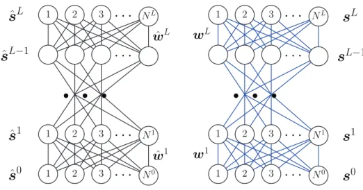
Following [16], we consider two coupled fully-connected DNN. One of them serves as the reference function under consideration, and the other as its perturbed counterpart, either in the weights or input variables. As shown in figure 1, each network consists of L + 1 layer; layer l has Nl _{neurons, which can be layer dependent. The reference network is parameterized}

by the weight variables1_{wˆl

}Ll=1, while the perturbed network is parameterized with {wl}Ll=1.

Similarly, variables with a circumflex are associated with the reference network. In the follow-ing, wl _{represents the N}l_×Nl−1 _{weight matrix at layer l, and w}l

i represents the Nl−1

dimen-sional weight vector of the ith perceptron at layer l. Denoting the input dimension as N = N0_,

we assume the sizes of all layers scale linearly with N as Nl_=αl_N.

A deterministic feed-forward network is defined by the recursive mapping _∀1lL hl i= √1 Nl−1 Nl−1 j=1 wl ijslj−1, (1) sl i=φlhli, (2) where _{wl

ij} are the weights, hli and sli are pre- and post-activation field and variable,

respec-tively, and φl(·) is the activation/transfer function at layer l. The scaling factor of 1/√Nl−1

in equation (1) is introduced for normalization. We primarily focus on networks with either sign [φs(x) =sgn(x)] or ReLU [φr(x) = max(x, 0)] activation functions in the hidden layers,

and consider binary input and output variables s0

i,sLi ∈ {1,−1} by applying the sign

activa-tion funcactiva-tion at the output layer sL

i =sgn(hLi) for a fair comparison across architectures. The

resulting feed-forward DNN implements a Boolean mapping f :{1,−1}N0→ {1,−1}NL, where each output node sL

is0 computes a Boolean function. In the following, we call the

two architectures sign-DNN and relu-DNN respectively, keeping in mind that sign activation function is always applied in the output layer.

To facilitate a path integral calculation, we consider stochastic dynamics between succes-sive layers. For the layer with sign activation function, the activation sl

i is disturbed by thermal

noise according to the following probability

1 2 3 _N0 1 2 1 2 3 _N1 NL 3 1 2 3 _N0 1 2 1 2 3 _N1 NL 3

· · ·

· · ·

· · ·

· · ·

· · ·

· · ·

· · ·

· · ·

· · ·

· · ·

ˆ

s

ˆ

s

ˆ

s

ˆ

s

s

s

s

s

ˆ

w

ˆ

w

w

w

Figure 1. The reference and perturbed fully-connected DNN, parameterized by {wˆl

} (black edges) and _{wl_{} (blue edges), respectively. Each layer l has N}l_=αl_{N nodes.}

frame-Psl i|hli(wl,sl−1)= expβsl ihli(wl,sl−1) 2coshβhl i(wl,sl−1) , (3) while for relu activation function, sl

i is disturbed by additive Gaussian noise Psl i|hli(wl,sl−1)= β 2πexp −β₂ sl i−φhli(wl,sl−1) 2 . (4) In the limit β_{→ ∞}, we recover the deterministic model. The evolution of the two systems follows the joint distribution

P(_{ˆsl i,sli}) =P(ˆs0,s0) L l=1 Nl i=1 Pˆsl i|ˆhli(ˆwl,ˆsl−1)Psli|hli(wl,sl−1). (5) To probe the difference between the functions implemented by the two networks, we feed in the same single input s0_{= ˆs}0 _{to the two systems such that P(ˆs}0_,s0_{) =P(ˆs}0₎N0

i=1δˆs0 i,s0i, and

study the resulting output difference due to parameter perturbation. For continuous weight variables, one useful choice for the weight perturbation is

wl ij=

1₋(ηl)2wˆlij+ηlδwlij,

(6) which ensures that wl

ij has the same variance of wˆlij as long as δwlij follows the same

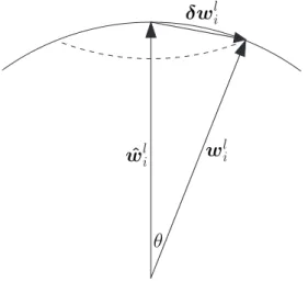
distribu-tion of wˆlij, and effectively rotates the high dimensional vector wˆil by an angle θl= sin−1ηl as

demonstrated schematically in figure 2.

In probing the sensitivity of a function due to input perturbations, the weights of two net-works are kept the same w= ˆw and a fixed fraction of input variables are flipped randomly. The resulting output difference of the two systems reflects the sensitivity and complexity of the underlying DNN.

ˆ

w

δw

w

θ

Figure 2. A geometric representation of perturbations on the parameter vector ˆwl i

defined in equation (6), resulting in a rotated vector wl

3. Generating functional analysis for typical behavior

Viewing the weights _{wˆlij,wlij} as quenched random variables, a generating functional analysis

has been proposed [16] to derive the typical behavior of DNN. It starts with computing the disorder-averaged generating functional

Γ( ˆψ,ψ) =Ewˆ,wEˆs,sexp −i l,i ( ˆψliˆsli+ψlisli) , (7) where the average _Eˆs,s is taken with respect to the joint probability equation (5). Assume the layer widths are the same Nl _{= N for all l. Upon averaging over the disorder wˆ,w, the} gener-ating functional can be expressed through a set of macroscopic order parameters such as the overlaps ql_=1/Nl iˆslisli and magnetizations mˆl=1/Nliˆsli,ml=1/Nlisli as Γ = {dqdQ. . ._}expNΨ(q,Q,. . .) (8) where Q is the conjugate variable of the order parameter q. In the large system size limit

N→ ∞, the generating functional Γ is dominated by the saddle point of the potential func-tion Ψ(q,Q,. . .). It gives rise to typical overlaps that dominate in probability, which facilitates analytical studies of random DNN.

Assume the weight perturbation follows the form of equation (6), and both weight and per-turbation are independent of each other and follow a Gaussian distribution wˆlij,δwijl ∼ N(0,σ2w).

It is found that for the layer with sign activation function in the limit β _{→ ∞}, the overlap evolves as [16]

ql₌ 2 πsin

−1_1−(ηl₎2_ql−1_{, 1lL.}

(9) Similarly, for ReLU activation function in the deterministic limit, if the weight standard devia-tion is chosen as σw=√2, the magnitude of the activations remains stable and the overlap

evolves as ql₌ 1 π 1−1−(ηl₎2_(ql−1₎2 +1−(ηl)2ql−1π 2 + sin−1 1−(ηl)2ql−1 _{, (10)}

while the output layer L follows equation (9) due to the use of the sign activation function. The restriction s0_{= ˆs}0 _{leads to q}0 _{= 1 in both cases.}

4. Large deviations in parameter sensitivity of functions

The generating functional analysis above gives typical behaviors of random DNN in the limit

N→ ∞. However, practical DNN always have finite sizes. Therefore, it is worthwhile to understand the deviation to the most probable behaviors under finite N. In the following, we adopt the large deviation analysis to tackle this problem. An introduction of large deviation theory and its application to statistical mechanics can be found in [30]. In essence, a continu-ous observable O in a system of size N (assumed to be large) is said to satisfy the large devia-tion principle if the probability of finding O follows

ProbN(O ∈[x,x+dx])e−NI(x)dx,

(11) where I(x) is the rate function of the observable. It implies that the probability density of O

scales as PN(O=x)e−NI(x), which is concentrated at the minimum of the rate function x∗_=argmin

xI(x) in large systems and the profile of I(x) quantifies the fluctuation of the

observable.

In this work the overlap of the output layer qL_:=1/NL

iˆsLisLi is at the focus of our study.

The path integral techniques adopted in the generating functional framework [16] can be adapted to tackle the large deviation analysis. We start with computing the probability density2

P(qL_{) =} δ ₁ NL i ˆsL isLi −qL =_Eˆw,wTrˆs,sP(ˆs0) N0 i=1 δ_s0 i,ˆs0i L l=1 P(ˆsl_|wˆl,ˆsl−1)P(sl_|wl,sl−1_)δ 1 NL i ˆ sL isLi −qL , (12) where the operation Trˆs,s is understood as an integration or summation depending on the nature of variables. The input distribution follows P(ˆs0) =_iP(ˆs0

i) =i(12δˆs0 i,1+

1 2δˆs0

i,−1). To deal

with the non-linearity of the pre-activation fields in the conditional probability, we introduce auxiliary fields _{ˆxl

i,xli} through the integral representation of delta-function

1= ∞ −∞ dˆ_hl idˆxli 2π e iˆxl i ˆ hl i−√1 Nl−1 jwˆlijˆslj−1 , 1= ∞ −∞ dhl idxil 2π e ixl i hl i−√1 Nl−1 jwlijslj−1 , (13) which allows us to express the quenched random variables wˆlij and wlij linearly in the

exponents, leading to P(qL) =_Eˆw,wTrˆs,sδ ₁ NLˆs L isLi −qL N0 i=1 P(ˆs0i)δs0 i,ˆs0i L l=1 Nl i=1 dˆ_hl idˆxli 2π dhl idxli 2π ×exp   L l=1 Nl i=1 logP(ˆsl i|ˆhli) + logP(sli|hli) +iˆxliˆhli+ixlihli   ×exp  ₋ L l=1 i √ Nl−1 Nl i=1 Nl−1 j=1 ˆ wl ijˆxliˆslj−1+wlijxlislj−1  . (14) Assuming self-averaging [31] we exchange the order of summation and integration, and first carry out the average over the disorder variables. Specifically, we consider the weights of the reference network to be independent and follow a Gaussian distribution wˆlij∼ N(0,σ2w) as

before, and three types of perturbations

2 _{Here we assume q}L_=1/NLNL

i=1ˆsLisLi to be a continuous variable by considering large NL. Instead, one can view qL _{as a discrete variable by definition (since the inputs are binary variables), where δ(·) should be understood as the}

(i) rotation of the weight vector wˆli following equation (6);

(ii) sparsification of the weight matrix wˆl by randomly dropping connections with probability

pl _{and rescaling the remaining weights by 1/1}

−pl to ensure the same weight strength

wl ij= _{0, with probabilityp}l_, 1 √₁ −plwˆ l ij, with probability 1−pl, (15) (iii) binarization of weight element wˆl

ij wl

ij=sgn(ˆwlij)σw,

(16) where σw is introduced for keeping the variance of wlij the same as wˆlij.

4.1. Macroscopic order parameters

For perturbation of type (i), the disorder average of the third line of equation (14) yields l,i exp −σ_w2 1 2(ˆxli)2 j(ˆslj−1)2 Nl−1 + 1 2(xli)2 j(slj−1)2 Nl−1 + 1−(ηl)2ˆxl ixli jˆslj−1slj−1 Nl−1 . (17) To decouple equations (14) and (17) over sites we introduce three sets of order parameters by inserting the identity

1= _dVˆl_dˆvl 2π/Nlei Nlˆ_Vl_[ˆvl₋1 Nl j(ˆslj)2]_{, 1= dV}l_dvl 2π/Nlei Nl_Vl_[vl₋1 Nl j(slj)2]_, 1= _dQl_dql 2π/Nlei Nl_Ql_[ql₋1 Nl jˆsljslj], _∀l₌L, (18)

and by expressing the output constraint as

δ ₁ NL NL i=1 ˆsLisLi −qL = _dQL 2π/NLeiN L_QL_[qL₋1 NL jˆsLjsLj]. (19) Upon introducing these macroscopic order parameters, equation  (17) becomes

l,iexp{−1/2[ˆxli,xli]·Σl·[ˆxli,xli]} with the covariance matrix Σl

Σl:=σ2w ˆ vl−1 _1−(ηl₎2_ql−1 1−(ηl)2ql−1 vl−1 . (20) The probability density in equation (14) involves Nl _{identical integration and summation at} each layer l, which can be performed individually [16], yielding

P(qL_{) =} dQL 2π/NL L−1 l=0 d_Vˆl_dˆvl 2π/Nl dVl_dvl 2π/Nl dQl_dql 2π/Nl ×eLl=−01Nl iˆVl_ˆvl_+iVl_vl_+iQl_ql_+NL_iQL_qL e−N0_iˆV0_+iV0_+iQ0 × L−1 l=1 dHle− 1 2(Hl)Σ−l 1Hl (2π)2_|Σl| Trˆsl,slP(ˆs l_|ˆhl_)P(sl_|hl_)e−iVˆl (ˆsl )2−iVl (vl )2−iQl ˆsl_sl Nl × dHLe− 1 2(HL)Σ−L1HL (2π)2|ΣL| TrˆsL_,sLP(ˆsL|ˆhL)P(sL|hL)e−iQ L_ˆsL_sL NL , (21)

where we have integrated out the auxiliary fields _{ˆxl,xl_} and introduced the field doublet

Hl_{:= [ˆh}l_,hl_{]. We further write P(q}L_{) as} P(qL) = _dQL 2π/NL L−1 l=0 d_Vˆl_dˆvl 2π/Nl dVl_dvl 2π/Nl dQl_dql 2π/Nl exp[−NΦ(Q,q,Vˆ,vˆ,V,v|qL)], (22) where ₋NΦ(Q,q,Vˆ,vˆ,V,v_|qL_{) is equal to the logarithm of the integrand in equation (21).}

Similar to the analysis in [16], the probability density P(qL_{) is dominated by the saddle point} (Q∗,q∗,. . .) of the potential function Φ(. . .) in the large N limit (Nl_=αl_{N with α}l _{as a}

constant)

P(qL₎

≈exp[₋NΦ(Q∗,q∗_{,. . .|q}L_)],

(23) where I(qL) = Φ(Q∗,q∗,. . .|qL_{) is the desired rate function.}

While this set-up is based on computing the deviation in function similarity with a single input qL_=1/NL

iˆsLisLi, one may argue that it requires testing on more than one input for

obtaining a robust estimation, e.g.

˜ qL_:= 1 NL_M M µ=1 NL i=1 ˆsL,µ i sLi,µ, (24) where M is the number of independent patterns used. Assuming that representation of differ-ent patterns are uncorrelated, we show in appendix C that for small M, the rate function I(˜qL₎

is approximately related to the single input case through a simple scaling

I(˜qL)_≈MΦ(Q∗,q∗,. . ._|˜qL).

(25) This assumption is valid for sign-DNN but not for relu-DNN. We also confirm this scaling relation by numerical experiments (see below and in appendix C).

4.2. Unifying three types of weight perturbations

The other two types of perturbations can be treated similarly. For network sparsification (15), the disorder average of equation (14) has the following form in the large Nl _{limit (see appendix} A for details) l,i exp −σ_w2 1 2(ˆxli)2 j(ˆslj−1)2 Nl−1 + 1 2(xli)2 j(slj−1)2 Nl−1 + 1₋pl_ˆxl ixli jˆslj−1slj−1 Nl−1 , (26)

which has the same form of equation (17) when pl _{is replaced by (η}l₎2_{. Introducing the same}

order parameters, we obtain the covariance of the fields ˆ_hl _{and h}l _{in the form of} Σsl :=σ2w ˆ vl−1 _1−pl_ql−1 1₋pl_ql−1 _vl−1 . (27) Hence, diluting connections with probability pl _{at layer l in a random DNN corresponds to} rotating each of the weight vector wˆli by an angle θl= sin−1pl.

Similarly, for network binarization in equation (16), the disorder average of equation (14) yields (see appendix B for details)

l,i exp −σ_w2 1 2(ˆxli)2 j(ˆslj−1)2 Nl−1 + 1 2(xli)2 j(slj−1)2 Nl−1 + 2 πˆx l ixli jˆslj−1slj−1 Nl−1 , (28) which corresponds to the covariance matrix of the fields ˆ_hl _{and h}l _{to be in the form}

Σbl :=σ2w   ˆv l−1 2 πql−1 2 πq l−1 _vl−1  . (29) Comparing to type (i) perturbation, one finds that binarizing weight elements in a random DNN corresponds to rotating each of the weight vectors wˆl_i by a fixed angle θl= cos−12

π ≈37◦. This phenomenon has been observed in [32] and is linked to the practical success of binary DNN. It is argued [32] that 37◦ _{is a very small angle in high dimensional spaces where two} randomly sampled vectors are typically orthogonal to each other; therefore weight binariza-tion approximately preserves the direcbinariza-tions of the high dimensional weight vectors, which contributes to the success of binary DNN.

Therefore, we establish that the three types of perturbations on random DNN can be unified in the same framework developed in section 4.1.

4.3. Saddle point equations

For networks with a generic activation function, the large deviation potential function Φ(. . .)

can be express as Φ =−α0iVˆ0(ˆv0−1) +iV0(v0−1) +iQ0(q0−1)− L−1 l=1 αl(iVˆlˆvl_+iVl_vl_+iQl_ql₎ −iQL_qL₋L l=1 αllog dˆ_hl_dhl_Trˆ sl_,slMl(ˆsl,sl,ˆhl,hl), (30) Ml(ˆsl_,sl_,hˆl_,hl_):= e− 1 2(Hl)Σ−l1Hl (2π)2|Σl| P (ˆsl_|ˆ_hl_)P(sl_|hl_)e−iˆ_Vl_(ˆsl₎2_−iVl_(vl₎2_−iQl_ˆsl_sl , 1l<L, (31) ML(ˆsL,sL,_hˆL_,hL_):= e− 1 2(HL)Σ−L1HL (2π)2|ΣL| eβˆsLˆ_hL 2cosh(βˆhL) eβsL_hL 2cosh(βhL₎e−i QL_ˆsL_sL , (32) where α0=1 since N0 _{= N.}

Setting the derivatives with respect to the conjugate order parameters ∂Φ/∂iVˆl, ∂Φ/∂iVl,

∂Φ/∂iQl to zero yields the saddle point equations ˆ v0_=v0_{=1, q}0_=1, (33) ˆ vl₌ dˆ_hl_dhl_Trˆ sl_,slˆsl2Ml(ˆsl,sl,ˆhl,hl) _dˆhldhlTrˆ sl_,slMl(ˆsl,sl,ˆhl,hl) =ˆsl2Ml, vl=sl2_Ml, 1l<L, (34) ql₌ dˆ_hl_dhl_Tr ˆsl_,slˆslslMl(ˆsl,sl,ˆhl,hl) dˆ_hl_dhl_Tr ˆsl_,slMl(ˆsl,sl,ˆhl,hl) =ˆslslMl, 1lL, (35) in which _Ml_(ˆsl_,sl_,hˆl_,hl_{) bears the meaning of an effective measure [33]. Notice that q}L _is an input parameter imposing a nonlinear end point constraint on iQL_{, which differs from the}

generating functional analysis calculation of typical behaviors [16], where qL _{is a dynamical} variable and iQL_{=0 at the saddle point.}

Setting ∂Φ/∂ql _{to zero yields the saddle point equations for the conjugate order parameters}

iQl iQl−1 ₌ αl αl−1 dˆ_hl_dhl_Tr ˆsl_,sl ∂ ∂ql−1Ml(ˆsl,sl,ˆhl,hl) _dˆhldhlTr ˆsl_,slMl(ˆsl,sl,ˆhl,hl) , 1lL. (36) Similar relations holds for i_Vˆl _{and iV}l_{. While the conjugate order parameters}

{Vˆl,Vl,Ql}

are defined on the real axis, they can be extended to the complex plane and evaluated on the imaginary axis in the saddle point approximation, in which case _{i_Vˆl_{, iV}l_{, iQ}l

} are real vari-ables. Other observables can be computed by resorting to the effective measure Ml once the saddle point is obtained, e.g. the mean activations are given by [33]

ˆ ml₌

ˆsl_Ml, ml=sl_Ml.

(37) Since the covariance matrix Σl(ql−1,. . .) depends on the order parameters of layer l − 1,

the effective measure Ml at layer l depends on the order parameters _{ql−1_{,. . .} of the previous}

layer, while it depends on the conjugate order parameters _{iQl_{,. . .}

} of the current layer. We then observe that the order parameters _{ql_{,. . .}

} propagate forward in layers, while _{iQl_{,. . .}

}

encoding the randomness leading to the desired deviation propagate backward, which resem-bles the structure in optimal control problem [34]. Therefore, we solve the saddle point equa-tions in a forward-backward iteration manner until convergence. Another feature to notice in equation (36) is the dependence of the saddle point solution on the layer-shape parameters

{αl_}, which does not play a role in the mean field solutions where all the conjugate order parameters _{iQl_{,. . .}

} vanish [16].

4.4. Explicit solutions for sign and ReLU activation functions

For networks with sign activation function the order parameters satisfy ˆvl_=vl_{=1, such that}

the only meaningful order parameters are {ql_,Ql_{}. The potential function Φ can be computed}

Φ(Q,q|qL_{) =−α}0_iQ0_(q0₋₁₎₋L l=1 αliQl_ql − L l=1 αllog cosh(iQl_)−sinh(iQl₎2 πsin −1_(1−(ηl₎2_ql−1_), (38) while the saddle point equations become

q0_=1,

(39)

ql₌ −sinh(iQl) + cosh(iQl)π2 sin−1(

1−(ηl)2ql−1)

cosh(iQl)₋sinh(iQl)_π2 sin−1(1₋(ηl)2ql−1₎ , ∀1lL,

(40)

iQl−1 ₌ π2sinh(iQl)

cosh(iQl)₋sinh(iQl)_π2sin−1(1₋(ηl)2ql−1₎

× α

l₁

−(ηl)2

αl−1_1−[1−(ηl₎2_](ql−1₎2, ∀1lL. (41)

Note that qL _{in equation (40) is an input parameter.}

For networks with ReLU activation function the potential function Φ also admits an explicit expression Φ(Q,q,Vˆ,ˆv,V,v|qL_{) =−α}0_iVˆ0_(ˆv0_{−1) +iV}0_(v0_{−1) +iQ}0_(q0₋₁₎ − L−1 l=1 αl(iVˆlˆvl_+iVl_vl_+iQl_ql_)−iQL_qL − L−1 l=1 αllog 1 2π_|Σl| 1 |Al_| π 2−tan−1 Al 12 |Al_| +1 |Bl_| π 2 + tan−1 Bl 12 |Bl_| + 1 |Σ−_l 1|  π 2−tan−1   Σ− 1 l,12 |Σ−_l 1|    +1 |Cl_| π 2+ tan−1 Cl 12 |Cl_|      −αLlog cosh(iQL_)−sinh(iQL₎2 πtan −1 ΣL,12 |ΣL| , (42)

where Al_,Bl_,Cl _{are 2×2 matrices defined as} Al_{= Σ}−1 l + _2iVˆl _iQl iQl _2iVl , Bl_{= Σ}−1 l + _{0 0} 0 2iVl , Cl_{= Σ}−1 l + _2iVˆl ₀ 0 0 . (43) The saddle point equations also admit a close-form expression accordingly.

5. Large deviations in input sensitivity of functions

In probing the sensitivity of a function to the flipping of input variables, the weights of two networks considered are taking the same values w=wˆ, which is done by setting ηl=0 in

equation (6). We constrain the input s0 _{of the perturbed system to have a pre-defined}

sensitivity of the output overlaps to input perturbations is investigated through the conditional probability P(qL|q0_{) =} P(qL,q0) P(q0) = δ 1 NL _iˆsLisLi −qL δ 1 N0_iˆs0is0i −q0 δ 1 N0_iˆs0_is0_i −q0 . (44) Without loss of generality, we choose a decoupled input distribution

P(ˆs0,s0_{) =} iP(ˆs0i)P(si0) =i(12δˆs0 i,1+ 1 2δˆs0 i,−1)( 1 2δs0 i,1+ 1 2δs0

i,−1) while the delta function

involving q0 _{in equation (44) constrains the systems to have the desired input correlation. The}

probability of input overlap P(q0_{) can be computed as}

P(q0) =Trˆs0_,s0 i P(ˆs0i)P(s0i) _dQ0 2π/N0ei N0_Q0_q0 −_N10iˆs0is0i = _dQ0 2π/N0 exp N0_iQ0_q0_{+ log cosh(iQ}0₎ ≈exp N0_iQ0∗_q0_{+ log cosh(iQ}0∗₎ =:exp₋NΦP(iQ0∗|q0), (45) ΦP(iQ0|q0):=−α0iQ0q0+ log cosh(iQ0), (46) iQ0∗_:=−tanh−1_(q0_), (47) where we have made use of the saddle point approximation of P(q0_{) in the large N}0 _{limit, with}

the corresponding potential function defined in equation (46) and the saddle point solution iQ0∗ _{given in equation (47).}

The computation of the joint probability P(qL,q0) is analogous to that of P(qL_{) in earlier} sections, P(qL,q0) =Ewˆ,wTrˆs,sP(ˆs0) N0 i=1 δs0 i,ˆs0i L l=1 P(ˆsl_|wˆl,ˆsl−1)P(sl_|wl,sl−1) × _dQ0 2π/N0 dQL 2π/NLe iN0_Q0_q0₋1 N0 iˆs0is0i +iNL_QL_qL₋ 1 NL iˆsLisLi = {dQdq. . ._}exp[₋NΦJ(Q,q,. . .|qL,q0)], (48) ΦJ=−α0iVˆ0(ˆv0−1) +iV0(v0−1) +iQ0q0+ log cosh(iQ0)−iQLqL − L−1 l=1 αl(iVˆlˆvl_+iVl_vl_+iQl_ql₎₋L l=1 αllog dˆ_hl_dhl_Tr ˆsl_,slMl(ˆsl,sl,ˆhl,hl). (49) The saddle point of iQ0 _{satisfies iQ}0∗_=−tanh−1_(q0_{), which coincides with the one of P(q}0₎

P(qL_|q0_{)≈exp−NΦ(Q}∗_,q∗_{,. . .|q}L_,q0_{)= exp−N(Φ}∗ J−Φ∗P) Φ(Q,q,. . ._|qL,q0) =₋α0iVˆ0(ˆv0₋1) +iV0(v0₋1)₋iQLqL − L−1 l=1 αl(iVˆlˆvl_+iVl_vl_+iQl_ql₎₋L l=1 αllog dˆ_hl_dhl_Tr ˆsl_,slMl(ˆsl,sl,ˆhl,hl), (50) where the saddle point solution _{Q∗_,q∗_{,. . .} have the same form as those in section 4.3,} except that q0 _{= 1 in equation (33) is replaced by the pre-defined value q}0 _{under investigation.}

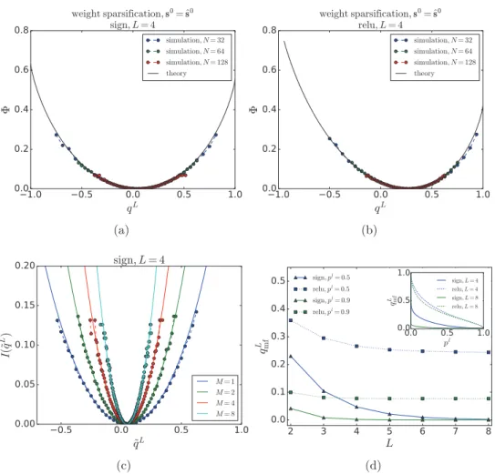
Figure 3. Weight sparsification of random DNN. In (a)_–(c), we set L = 4 and pl _{= 1/2;}

solid lines correspond to theory while dashed lines with circle markers correspond to estimation from simulation. The estimation of the rate function from simulations are obtained by 100 000 samples and the corresponding curve has been shifted such that the minimum is at zero. (a) The rate function Φ versus qL _{for sign activation function.}

(b) The rate function Φ versus qL _{for ReLU activation function. (c) The rate function}

I(˜qL_{) of output overlap ˜q}L _{defined by M patterns; the theoretical results are given by}

equation (25), while the simulation results are obtained on systems with N = 64. (d) Mean field solutions of output overlap qL

mf as a function of system depth L. Inset: qLmf versus pl _{for different depths.}

6. Results

6.1. Weight sparsification

We first consider the effect of weight perturbation by sparsifying connections as in equa-tion (15). For a concrete example, we consider DNN with L = 4, uniform layer width αl=1

and disconnection probability pl _{= 1/2, for which we compute the large deviation rate} func-tion I(qL) = Φ(Q∗,q∗_{,. . .|q}L_{) by solving the saddle point equation in section 4.3 and}

com-pare it to numerical experiments. For relu-DNN, we always set σw=√2. The results are

shown in figures 3(a) and (b), which exhibit a perfect match between the theory and simula-tion. The most probable qL_{, located at the minimum of Φ corresponds to the mean field} solu-tion, where qL

mf≈0.047 for sign-DNN and qLmf≈0.266 for the relu-DNN. However, in finite

systems they have a non-zero probability of admitting a higher value of qL _{due to fluctuations.} We can compute the probability from the rate function by P(qL) = exp(₋NΦ∗_(qL_))/Z3 _and estimate the tail probability of output mismatch. As an example we consider N = 64 and find that P(qL>1/2)_≈0.055% for sign-DNN and P(qL>1/2)_≈3.8% for relu-DNN, which is non-negligible especially for ReLU activation4_.

In figure 3(c), we also demonstrate that the approximation of rate function I(˜qL) of output overlap ˜qL, estimated for M patterns by employing equation (25), is accurate for DNN with sign activation, while the approximation does not hold for deep ReLU networks (see appendix C). Therefore in sign-DNN, the probability of finding perturbed DNN agreeing on all M patterns with the reference DNN decays exponentially with M (at least for small M values). This may not be the case in relu-DNN which requires further exploration in a future study.

In figure 3(d), we compare the mean field output overlaps qL

mf between DNN with sign and

ReLU activations for different system depths and disconnection probability pl_{. It is shown} that relu-DNN are more robust to weight sparsification perturbation, as expected; the per-turbed relu-DNN have residual correlations with the reference networks even after removing 90% of the weights. The robustness of relu-DNN to weight dilution was also observed and theoretically analysed in [35]. Finally, we remark that our scenario is different from the practi-cal methods used to prune networks trained on specific data; in this case particular heuristic rules have been developed to disconnect weights instead of the random removal used here. The success of weight pruning in practice hightlights the weight-redundancy in real trained networks [24, 35] but may also be influenced by properties of the data used and training meth-ods. This behaviour is absent in random networks with random data, as indicated in the inset of figure 3(d), where even a small dilution probability can deteriorate the overlap. Additional modelling considerations are needed to address practical scenarios.

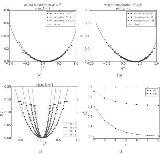
6.2. Weight binarization

We then consider the effect of perturbation by binarization of weight variables as in equa-tion (16). Also here we consider uniform layer width αl=1. The results shown in figure 4, 3 _{For finite N}L_{, the output overlap is a discrete variable q}L_{∈ {1, 1−} 2

NL, 1−_N4L,. . .,−1}, so it is convenient to

consider the discretized probability distribution of qL _{as Prob(q}L_{) =P(q}L_)∆qL_{= exp(−NΦ}∗_(qL_{))/Z; the}

normal-ization constant is computed as Z=_kexp(−NΦ∗_(qL

k))∆qL, where the summation runs over all possible values

of qL _{and ∆q}L₌ 2

NL. Although we could not find the saddle point solution of Φ(. . .|qL) in the vicinity of qL = −1

for relu-DNN (see figure 3(b)), the contribution from that region to the cumulative probability of the overlap is negligible .

4 _{Notice that such estimation is obtained by saddle point approximation in equation (22) and by keeping the leading} order contribution, which may be slightly biased for small N.

are very similar to the effect of weight sparsification. As pointed out in section 4.2, bina-rizing weights of random DNN corresponds to rotating the weight vector wˆl_i by an angle

θl= cos−1_π2 [32], or equivalently, disconnecting weights with a particular probability

pl₌₁₋ 2

π. The matches between theory and simulation in figures 4(a)–(c) validates the large deviation-based analysis in both sign and relu-DNN and the scaling relation of equation (25) in sign-DNN. The relu-DNN are more biased to the regime of positive correlation and more robust to binarizing perturbation as seen in figure 4(d).

6.3. Sensitivity to input perturbation

We have shown that relu-DNN with random weights are robust to parameter perturbations such as weight sparsification and weight binarization, which is a desired property for better

Figure 4. Weight binarization of random DNN. (a) Φ versus qL _{for sign activation}

function. (b) Φ versus qL _{for ReLU activation. (c) The rate function I(˜q}L_{) of output}

overlap ˜qL _{defined by M patterns; solid lines are theoretical results while dashed lines}

with circle markers are estimated by simulation. (d) Mean field solutions of output overlap qL

generalization. On the other hand, such network ensembles typically represent simple func-tions as studied in [21, 22]. The simplicity of the functions generated is one reason accounting for the observed robustness to parameter perturbation.

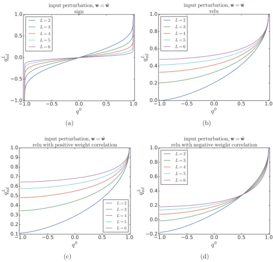
To probe the function complexity, we study the function sensitivity under input perturba-tion while keeping w= ˆw [28]. Flipping n input variables corresponds to the input overlap

q0₌₁₋ 2n

N0. In figures 5(a) and (b) we depict the overlap qL_mf of the final output as a

func-tion of input overlap q0 _{(keeping in mind that we always apply the sign activation in the}

output layer). While the outputs become more de-correlated in deeper layers of sign-DNN, the relu-DNN induce correlation at deeper layers. Therefore, random relu-DNN tend to forget the input structure at deeper layers, generating increasingly simpler functions that are robust to parameter perturbation. This phenomenon has been noticed in the Gaussian process-like analysis of DNN [10_–12].

Figure 5. Mean field solutions qL

mf versus q0 in the scenario of input perturbation where w= ˆw. In all architectures, sign activation function is applied at the output layer. (a) DNN with sign activation functions and uncorrelated random weights. (b) DNN with ReLU activation at the hidden layers, with uncorrelated random weights, and sign activation at the output layer. (c) Relu-DNN with positive weight correlation c=2/(3N). (d) Relu-DNN with negative weight correlation c=−2/(3N).

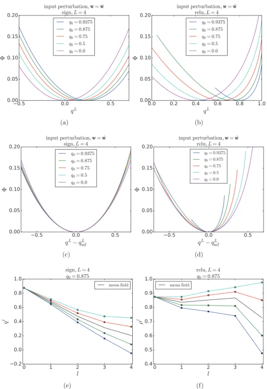
Figure 6. Large deviation of output similarity qL _{under input perturbation where}

w= ˆw. Sub-figures (c) and (d) are the same as (a) and (b), except for the shifted x -coordinates. (a) and (b) Φ versus qL _{for sign- and relu-DNN, respectively. (c) and (d) Φ}

In [16], we investigated the effect of weight correlation in the form of

P(ˆwl_i) = exp(₋1₂(ˆwl_i)_A−1_wˆl i)/

(2π)Nl−1

|A|, with A=σw2(I−cJ) where I is the identity

matrix and J the all-one matrix. We found that DNN with ReLU activation functions and nega-tive weight correlation c < 0 are more sensitive to parameter perturbation. Here we examine the sensitivity of relu-DNN to input perturbation by employing the same results developed in [16]. In figures 5 (c) and (d), we depict the mean field output overlap qL

mf as a function of input

overlap q0_{. It is observed that negative weight correlation corresponds to a higher sensitivity to}

input perturbation, indicating that the relu-DNN with negatively correlated weights generate more complex functions than those with random or positively correlated weights. We con-jecture that negative weight correlation develops in very deep ReLU networks when they are trained to performed complex task where a high expressive power is needed, a phenomenon that has been observed in [36].

In figure 6, we further investigate deviations from the typical behaviors in the presence of input perturbations for the specific example with L=4,αl=1. The rate functions Φ(qL)

depicted in figures 6(a) and (b) dictate the rate of convergence to the typical behaviors with increasing N by the large deviation principle, for both sign and ReLU activations, respectively. In figure 6(c), we observe that the rate functions have similar trends in the vicinity of the mean field solution qL

mf for different levels of input perturbation (corresponding to different q0) in

sign-DNN, while they are more distinctive in relu-DNN as seen in figure 6(d). In relu-DNN, smaller input perturbation (larger q0_{) leads to smaller variance of q}L _{around q}L

mf. The rate

func-tion of relu-DNN is also more asymmetric around qL

mf, suggesting that large deviations will be

more often observed below qL

mf than above it. This indicates that random relu-DNN of finite

size may produce functions that are slightly more complex than what would be expected by the mean field solutions, which remains to be verified.

We also examine the dominant trajectories across layers leading to particular deviations by monitoring the correlations of activations between the two systems across layers. The relevant quantity is the correlation coefficient

ρl= q l −mˆl_ml ˆ vl_{−( ˆm}l₎2_vl_−(ml₎2, (51) where the mean activations mˆl and ml _{are computed by equation (37). We find that sign-DNN} satisfy mˆl=ml=0,ˆvl_=vl_{=1, such that ρ}l_=ql _{in this case. The results are shown in}

fig-ures 6(e) and (f), which suggest that the deviations of qL _{from the typical value q}L

mf are mainly

contributed by the deviations at later layers.

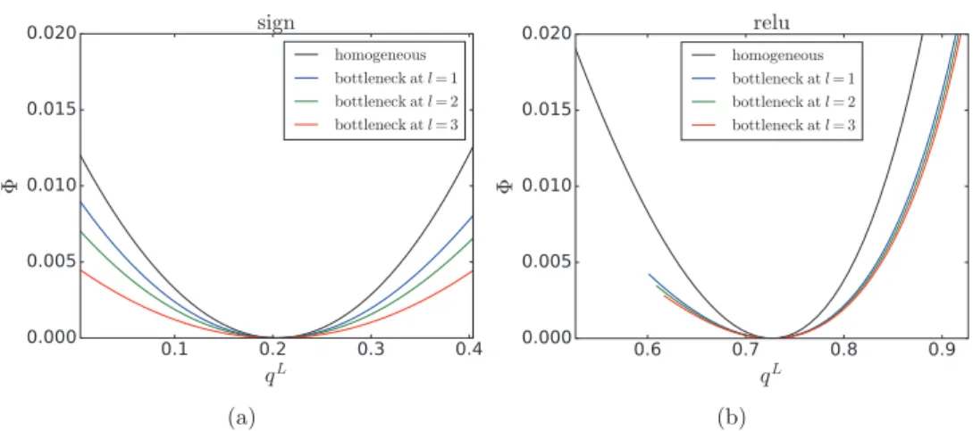
Lastly, we investigate the effect of DNN architecture on the deviation. In particular, we con-sider a single bottleneck layer at a particular hidden layer l _{(0<l<L) with α}l

=1₈ while all other layers satisfy αl=1,_∀l=l_{. Placing the bottleneck at later layer introduces a higher} variability of output overlap qL _{by observing smaller values of the rate function in figure 7; this} effect is more prominent in sign-DNN, while it is much less noticeable in relu-DNN.

7. Discussion

By utilizing the large deviation theory coupled with the path integral analysis, we derive the sensitivity of finite size random DNN under parameter and input perturbations. Random DNN with sign or ReLU activation function are shown to satisfy the large deviation principle, where the rate functions govern an exponential decay of the deviation to the mean field behaviors as the size of the system increases. We also investigate the effects of weight sparsification and binarization of random DNN, and uncover their equivalence to rotation of weight vector in high dimension. Random DNN with ReLU activation function are found to be robust to these parameter perturbations, which is caused by the low complexity of the corresponding function mappings. Random initializing the weights of ReLU DNN places a prior for simple functions, while they have the capacity to compute more complex functions with specifically trained weights. The next important question is how the networks adapt to perform complex tasks by the training processes.

Acknowledgments

BL and DS acknowledge support from the Leverhulme Trust (RPG-2018-092), European Union_’s Horizon 2020 research and innovation programme under the Marie Sk_ł odowska-Curie Grant agreement No. 835913. DS acknowledges support from the EPSRC programme Grant TRANSNET (EP/R035342/1).

Appendix A. Disorder average for weight sparsification

For network sparsification (15), the disorder average in equation (14) can be computed as

Figure 7. Effect of a single bottleneck layer on the rate function in the scenario of input perturbation. The bottleneck layer l _{has width parameter α}l

=1₈ while all other layers have αl=1. (a) Sign-DNN. (b) relu-DNN.

Ewˆ l,i,j exp −i √ Nl−1wˆ l ijˆxliˆslj−1 (1−pl_{) exp} −i √ Nl−1_1−plwˆ l ijxlislj−1 +pl = l,i,j (1−pl_{) exp−} σw2 2Nl−1 ˆxliˆslj−1+xlislj−1/ 1−pl 2 +plexp − σ 2 w 2Nl−1 ˆ xl iˆslj−1 2 = l,i,j (1−pl₎₁ − σ 2 w 2Nl−1 ˆ xl iˆslj−1+xlislj−1/ 1−pl 2 +pl₁ − σ 2 w 2Nl−1 ˆ xl iˆslj−1 2 +O ₁ (Nl−1₎2 ≈ l,i,j 1− σ 2 w Nl−1 ₁ 2(ˆxli)2(ˆslj−1)2+ 1 2(xli)2(slj−1)2+ 1−pl_(ˆxl ixli)(ˆslj−1slj−1) ≈ l,i exp −σ_w2 ₁ 2(ˆxli)2 j(ˆslj−1)2 Nl−1 + 1 2(xli)2 j(slj−1)2 Nl−1 + 1−pl_ˆxl ixli jˆslj−1slj−1 Nl−1 , (A.1)

where we have made use of the large Nl _{approximation.} Appendix B. Disorder average for weight binarization

For weight binarization in (16), the disorder average in equation (14) can be computed as Eˆw l,i,j exp −i √ Nl−1 ˆ wl ijˆxliˆslj−1+sgn(ˆwlij)σwxlislj−1 = l,i,j 0 −∞ dwˆl ijN(ˆwlij|0,σ2w) exp −i √ Nl−1 ˆ wl ijˆxliˆslj−1−σwxlislj−1 + ∞ 0 d ˆ wl ijN(ˆwlij|0,σw2) exp −i √ Nl−1 ˆ wl ijˆxliˆslj−1+σwxlislj−1 = l,i,j exp − σ 2 w 2Nl−1(ˆxli)2(ˆslj−1)2 ₁ 2 1+erf _iˆxl jˆslj−1σw 2√Nl−1 exp _ixl islj−1σw √ Nl−1 + 1−erf _iˆxl jˆslj−1σw √ 2Nl−1 exp _−ixl islj−1σw √ Nl−1 = l,i,j exp − σ 2 w 2Nl−1(ˆxli)2(ˆslj−1)2 ₁ 2 1+_√2 π iˆxl jˆslj−1σw √ 2Nl−1 1+ix l islj−1σw √ Nl−1 − 1 2 (xl islj−1σw)2 Nl−1 + 1−√2_πiˆx l jˆslj−1σw √ 2Nl−1 1−ix l islj−1σw √ Nl−1 − 1 2 (xl_isl_j−1σw)2 Nl−1 +O ₁ (Nl−1₎2 ≈ l,i,j exp − σ 2 w 2Nl−1(ˆxli)2(ˆslj−1)2 1− σ_w2 Nl−1 ₁ 2(xli)2(slj−1)2+ 2 π(ˆx l ixli)(ˆslj−1slj−1) ≈ l,i exp −σ_w2 ₁ 2(ˆxli)2 j(ˆslj−1)2 Nl−1 + 1 2(xli)2 j(slj−1)2 Nl−1 + 2 πˆx l ixli jˆslj−1slj−1 Nl−1 , (B.1)

where the large Nl _{approximation has been employed.}

Appendix C. Large deviation in the multiple-pattern scenario Consider function similarity estimated for multiple patterns

˜ qL₌ 1 M M µ=1 ₁ NL NL i=1 ˆsL_i,µsL_i,µ =: 1 M M µ=1 qL,µ (C.1) where ˆsL_i,µ(ˆs0,µ) is the ith output of the reference network with the µth input ˆs0,µ drawn indepen-dently and identically from the input distribution P(s0). In the small fluctuation regime, where

each qL,µ _{is close to the mean field solution q}L

mf, we have I(qL,µ)≈1/2I(qLmf)(qL,µ−qLmf)2

(both I(qL_mf) and I(q_mfL ) vanish [30]), i.e. P(qL,µ_{) can be approximated by a Gaussian density}

P(qL,µ)_∼exp −N₂I(qL_mf)(qL,µ₋qL_mf)2 , (C.2) where the corresponding variance is 1/(NI_(qL

mf)). Since the M inputs are independent, we

also assume the outputs are also approximately independent (which holds in sign-DNN but does not necessary for relu-DNN since ReLU non-linearity can induce correlations among variables), such that the variance of ˜qL is 1/(MNI_(qL

mf)). Therefore, in the vicinity of qLmf we

have

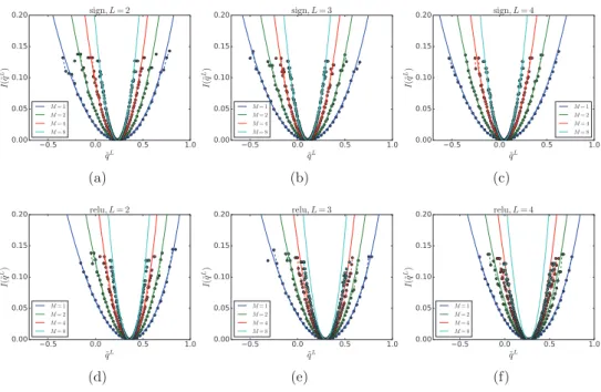
Figure C1. The rate function I(˜qL_{) of output overlap ˜q}L _{defined for M patterns and}

DNN with different activation functions and system depths, in the scenario of weight sparsification with disconnection probability pl _{= 1/2. Solid lines correspond to}

theoretical results and dashed lines with circle markers correspond to estimation from simulation.

P(˜qL)_∼exp −MN₂ I(qL_mf)(˜qL₋qL_mf)2 , (C.3) implying that the corresponding rate function differs from the one with single pattern by a factor of M.

More formally, one can directly compute the probability density P(˜qL_{) as} P(˜qL_{) =} δ ₁ MNL µ,i ˆsL,µ i sLi,µ−˜qL =_Eˆw,wTrˆs,sδ ₁ MNL µ,i ˆ sL,µ i sLi,µ−˜qL µ,i P(ˆs0,µ i )δs0,µ i ,ˆs0,iµ µ,l,i dˆ_hl,µ i dˆxli,µ 2π dhl,µ i dxli,µ 2π ×exp   µ,l,i logP(ˆsl,µ i |ˆhli,µ) + logP(sil,µ|hli,µ) +iˆxli,µˆhli,µ+ixli,µhli,µ   ×exp  ₋ µ,l i √ Nl−1 i,j ˆ wl ijˆxli,µˆslj−1,µ+wlijxli,µslj−1,µ  . (C.4)

Since the weights _{wˆlij,wlij} are shared among the M patterns, average over these variables on

the last line of equation (C.4) leads to coupling between patterns on the pre-activation fields l,i exp   −σ 2 w µ,ν ₁ 2ˆxl, µ i ˆxli,ν_N1l−1 j ˆsl−1,µ j ˆslj−1,ν+1₂xil,µxli,ν_N1l−1 j sl−1,µ j slj−1,ν + 1−(ηl)2ˆx_il,µxl_i,ν 1 Nl−1 j ˆsl_j−1,µsl_j−1,ν _ . (C.5)

By introducing the following overlap matrices as macroscopic order parameters

ql,µν ₌ 1 Nl j ˆsl,µ j slj,ν, ˆvl,µν= _N1l j ˆsl,µ j ˆslj,ν, vl,µν = _N1l j sl,µ j slj,ν. (C.6) Equation (C.4) can be factorized over sites as before. However, we have O(LM2_{) order}

param-eters here, while there are only O(L) order parameters in the single pattern case. To further simplify the calculation, we assume a symmetric structure of the cross-pattern overlaps at the saddle point ql,µν _=ql,_δ

µν+ql,⊥(1−δµν), where ql,,ql,⊥ are the diagonal and off-diagonal matrix elements respectively. Under this assumption, one can in principle evaluate the integral in (C.4), but the resulting calculation becomes rather involved.

Alternatively, since the M input patterns are independent, we expect the diagonal ele-ments of the matrix ql,µν _{to be larger than the off-diagonal elements (sum of correlated} variables versus sum of random variables). In particular, for sign activation we expect

ql,_∼O(1),ql,⊥_∼O(√1

Nl) since q

l,⊥ _{involves a summation over weakly correlated} posi-tive and negaposi-tive numbers. We therefore approximate the summation µν[. . .] in the expo-nential of equation  (C.5) by _µ=ν[. . .], which yields MNl _{un-coupled identical integrals} at each layer Nl_{. It eventually leads to the rate function of multiple-pattern overlap ˜q}L _as I(˜qL)≈MΦ(Q∗,q∗,. . .|q˜L), where Φ(Q∗,q∗,. . .|qL_{) is the rate function of the single-pattern}