Contents lists available atScienceDirect
International Journal of Approximate Reasoning
j o u r n a l h o m e p a g e :w w w . e l s e v i e r . c o m / l o c a t e / i j a rCore-generating approximate minimum entropy discretization for rough
set feature selection in pattern classification
David Tian
a,b,∗, Xiao-jun Zeng
b, John Keane
baDepartment of Computing, Faculty of ACES, Sheffield Hallam University, Howard Street, Sheffield S1 1WB, UK bSchool of Computer Science, University of Manchester, Oxford Road, Manchester M13 9PL, UK
A R T I C L E I N F O A B S T R A C T
Article history:
Received 15 June 2009 Revised 14 November 2010 Accepted 3 March 2011 Available online 21 March 2011
Keywords:
Core-generating approximate minimum entropy discretization
Rough set feature selection Pattern classification
Constraint satisfaction optimization problems
Rough set feature selection (RSFS) can be used to improve classifier performance. RSFS re-moves redundant attributes whilst retaining important ones that preserve the classification power of the original dataset.Reductsare feature subsets selected by RSFS.Coreis the inter-section of all the reducts of a dataset. RSFS can only handle discrete attributes, hence, contin-uous attributes need to be discretized before being input to RSFS. Discretization determines thecoresize of a discrete dataset. However, current discretization methods do not consider thecoresize during discretization. Earlier work has proposed core-generating approximate minimum entropy discretization (C-GAME) algorithm which selects the maximum number of minimum entropy cuts capable of generating a non-emptycorewithin a discrete dataset. The contributions of this paper are as follows: (1) the C-GAME algorithm is improved by adding a new type of constraint to eliminate the possibility that only a single reduct is present in a C-GAME-discrete dataset; (2) performance evaluation of C-GAME in compari-son to C4.5, multi-layer perceptrons, RBF networks and k-nearest neighbours classifiers on ten datasets chosen from the UCI Machine Learning Repository; (3) performance evalua-tion of C-GAME in comparison to Recursive Minimum Entropy Partievalua-tion (RMEP), Chimerge, Boolean Reasoning and Equal Frequency discretization algorithms on the ten datasets; (4) evaluation of the effects of C-GAME and the other four discretization methods on the sizes of reducts; (5) an upper bound is defined on the total number of reducts within a dataset; (6) the effects of different discretization algorithms on the total number of reducts are analysed and (7) performance analysis of two RSFS algorithms (a genetic algorithm and Johnson’s algorithm).
© 2011 Elsevier Inc. All rights reserved.
1. Introduction
Pattern classification is an important task in data mining [34–36,23–26]. The curse of dimensionality is a major bottleneck in the classification of high dimensional patterns. High dimensional datasets often contain redundant features that do not contain useful information for pattern classification. This may result in relatively low performance of classifiers obtained using all features. In addition, for high dimensional datasets, learning classifiers of high performance often requires a large number of patterns. The higher the dimensionality of the datasets, the more patterns are required to obtain classifiers with high classification performance. When the number of available patterns is small, the classification performance of the classifiers obtained using the available training patterns is also likely to be poor. Feature selection removes redundant features from the set of all features while keeping all important features [2], thus helping to alleviate the curse of dimensionality.
∗Corresponding author at: Department of Computing, Faculty of ACES, Sheffield Hallam University, Howard Street, Sheffield S1 1WB, UK. E-mail addresses:[email protected]; [email protected] (D. Tian), [email protected] (X.-j. Zeng), [email protected] (J. Keane). 0888-613X/$ - see front matter © 2011 Elsevier Inc. All rights reserved.
Feature selection may also help to improve the performance of other data mining methods e.g. clustering and regression. The two main types of feature selection approaches arefilterandwrapperapproaches [28]. Filters select features based on datasets properties and can be used as pre-processors of classifier learning algorithms. Wrappers select features based on the classification performances of classifiers. Feature selection using rough set theory [1,6–12] is a well-established filter approach. However, rough set feature selection (RSFS) handles discrete attributes only. To handle continuous datasets, discretization can be performed as a pre-processor of RSFS to transform continuous datasets to discrete datasets which are input to RSFS.
Discretization methods have been widely studied [13,20,22] and can be categorized on three axes: global vs. local meth-ods, supervised vs. unsupervised and static vs. dynamic [13]. Local methods such as Recursive Minimal Entropy Partitioning (RMEP) [13], discretize one attribute at a time based on a subset of instances of the dataset. Global methods such as Boolean Reasoning [14] consider all attributes before deciding which one to discretize based on all instances of the dataset. Super-vised methods such as 1RD [13] and ChiMerge [13] make use of class labels during discretization, whereas unsupervised methods such as Equal Width Intervals (EWI) and Equal Frequency Intervals (EFI) do not make use of the class labels. Static methods such as RMEP and 1RD discretize each attribute independently of the other attributes. Dynamic methods take into account the interdependencies between all attributes of a dataset [21].
RSFS selects reducts: minimal feature subsets that preserve the classification power of the dataset. For a given dataset, there exists numerous reducts.Coreis the set of all the common attributes of all the reducts, socoredetermines some of the attributes within each reduct. Therefore,corecritically affects the sizes of the reducts and may also critically affect the classification performance of the classifier learnt from the reduced dataset using the reduct. Ifcorecontains the significant attributes for object classification, each reduct will contain the significant attributes. If, however,coredoes not contain some significant attributes, some reducts may not contain significant attributes. Discretization determines thecoreof a discrete dataset, socorecan be considered as a property of a discrete dataset. However, none of the current methods usescoreas a criterion for discretization; RMEP discretizes data based on entropy of cuts; ChiMerge discretizes data based on
χ
2, a statistic measure of two adjacent intervals; Boolean Reasoning discretizes a dataset using the discernibility of cuts; EWI and EFI discretize data using interval width and frequency count respectively; 1RD discretizes each attribute so that a majority class exists for each interval of each attribute.Recent research on rough sets has been mainly concerned with their extension e.g. Gaussian kernel-based fuzzy rough sets (GKFRS) [33], covering generalized rough sets [32] and attribute dependency functions [31]. This paper extends the core-generating approximate minimum entropy discretization (C-GAME) algorithm which selects the maximum number of minimum entropy cuts capable of generating a non-emptycorewithin a discrete dataset [29]. Covering generalized rough sets and attribute dependency functions handle only discrete datasets. GKFRS is capable of handling both continuous and discrete datasets. Yang and Li [32] have redefined approximation spaces of covering generalized rough sets, where the concept of covering is an extension of the concept of a partition in rough sets. Reduction procedures for covering generalized rough sets have also been proposed [32,30]. Attribute dependency functions are based on a decision-relative discernibility matrix [31]. These functions measure how many times condition attributes are used to determine the decision value. Data efficiency is considered in the computation of dependency degrees. GKFRS is a hybrid model which combines Gaussian kernel functions with fuzzy rough set models and uses Gaussian kernel functions to extract fuzzy similarity relations between samples for fuzzy rough set-based data analysis. Gaussian kernels are used to compute fuzzy relations in fuzzy rough sets and approximate arbitrary fuzzy subsets with kernel induced fuzzy granules.
The C-GAME algorithm was proposed in our previous work [29]; in comparison, the contributions of this paper are as follows:
•
The C-GAME algorithm is improved by adding a new type of constraint to eliminate the possibility that only a single reduct is present in a C-GAME-discrete dataset.•
C4.5, multilayer-perceptrons, RBF neural networks and K-Nearest Neighbors classifiers are used here to evaluate the performance of C-GAME on 10 datasets including Ionosphere and SPECTF datasets; the earlier work only uses C4.5 and Ionosphere, and SPECTF datasets to evaluate C-GAME.•
Performance comparison of the C-GAME algorithm with four discretization algorithms: Recursive Minimum Entropy Partition (RMEP), Chimerge, Boolean Reasoning and Equal Frequency methods, is given here in terms of the accuracy of the four classifiers for the afore-mentioned 10 datasets; the earlier work only uses RMEP and Ionosphere, and the SPECTF datasets for comparison.•
The effects of C-GAME and the above four discretization algorithms on the sizes of reducts are analysed.•
An upper bound (UB) is defined on the total number of reducts within a dataset in terms of Cartesian products and ordered m-tuples, whereas [29] only briefly mentions its existence without definition.•
For each of the 10 datasets used here, the effects of C-GAME and the above four discretization algorithms on the total number of reducts are analysed.•
Both the relationships between the speed of a genetic algorithm and the total number of reducts and between the speed of Johnson’s algorithm and core size are analysed here.The paper is structured as follows: Section2presents preliminary concepts; C-GAME is presented in Section3; Section4 provides performance evaluation of C-GAME; and conclusions are presented in Section5.
2. Preliminary concepts
2.1. Rough set theory
Let
A
=
(
U,
A∪ {
d}
)
be a decision table whereUis a finite set of objects (the universe),Ais a non-empty set of condition attributes; anddis the decision attribute. For anyB⊆
A, the indiscernibility relationIND(
B)
[1] is defined as follows:IND
(
B)
= {
(
x,
x)
∈
U2|∀
a∈
B a(
x)
=
a(
x)
}
.
(1)If
(
x,
x)
∈
IND(
B)
, then objectsxandxare indiscernible from each other usingB. The indiscernibility relation generates a partition of the universeU, denotedU/
IND(
B)
[1]:U
/
IND(
B)
= {[
x]
IND(B):
x∈
U}
,
(2)where
[
x]
IND(B)is the equivalence class of IND(B). In particular, the elements ofU/
IND(
{
d}
)
are called decision classes [1]. LetXibe theith decision class, the lower approximationBXiofXiusing B is defined [1]:BXi
=
{
Y∈
U/
IND(
B)
:
Y⊆
Xi}
.
(3) The positive regionPOSB(
d)
contains all objects ofUthat can be certainly classified to the decision classes using the knowledge inB[1]:POSB
(
d)
=
Xi∈U/IND(d)BXi
.
(4)A subset of featuresB
⊆
Ais called a reduct, ifBsatisfies the following conditions: [1]:POSB
(
d)
=
POSA(
d)
(5)POSB−{i}
(
d)
=
POSB(
d),
∀i
∈
B.
(6)Hence, a reduct is a minimal feature subset preserving the positive region ofA. For a decision table
A
, there often exists numerous reducts.Coreis defined to be the intersection of all the reducts ofA
. Therefore,corecontains all indispensable features ofA. The discernibility matrixMis defined as [1]:M
=
(
cijd),
where c d ij= ∅
,
ford(
xi)
=
d(
xj)
cijd=
cij,
ford(
xi)
=
d(
xj)
,
(7) cij= {
a∈
A:
a(
xi)
=
a(
xj)
}
,
(8)wherecijis a matrix entry.Corecan be computed as the set of all singletons of the discernibility matrix of the decision table:
core
= {
a∈
A:
cij= {
a}
,
for some i,
j∈
U}
,
(9)wherecijis a matrix entry. TheB-information function is defined as [14]:
InfB
(
x)
= {
(
a,
a(
x))
:
a∈
B,
B⊆
A for x∈
U}.
(10)The generalized decision
∂
BofA
is defined as follows [14]:∂
B:
U→
2Vd,
(11)where
∂
B(
x)
= {i
: ∃x
∈
U[(
x,
x)
∈
IND(
B)
∧
d(
x)
=
i]} (12) and 2Vd is the power set ofVd. A discernibility function (df) is defined based on the discernibility matrix. It is a Boolean functionfwithmBoolean variablesa∗1
,
a∗2, . . . ,
a∗mcorresponding to the attributesa1,
a2, . . . ,
amof the decision table [1]: f(
a∗1, . . . ,
a∗m)
= ∧{∨
(
c∗ij)
:
1≤
j≤
i≤ |
U|
,
cij= ∅}
,
(13) wherec∗ij= {
a∗|
a∈
cij}
. A df can be simplified by removing its duplicate clauses1and the clauses that include other clauses. LetPdenote the conjunction of a smallest subset of the Boolean variablesa∗1, . . . ,
a∗msuch that assigning the value true to1 ∨(
Fig. 1. An example discernibility function.
each of the variables results inf
(
a∗1, . . . ,
a∗m)
evaluating to true.Pis called a prime implicant off(
a∗1, . . . ,
a∗m)
.Pcorresponds to a reduct. An example discernibility functiondfand its simplified discernibility functiondfare shown in Fig.1.2.2. Discretization
In [19], discretization problems are defined as follows. Let
A
=
(
U,
A∪ {d}
)
be a decision table whereUis a finite set of objects (the universe),Ais a non-empty finite set of condition attributes such thata:
U→
Va(Va, the set of values ofa) for alla∈
Aanddis the decision attribute such thatd:
U→
Vd(Vd, the set of values ofd). It is assumed thatVa= [
la,
ra)
⊂
R
whereR
is the set of real numbers. In discretization problems, it is assumed thatA
is a consistent decision table. That is,∀
(
oi,
oj)
∈
U×
U, ifd(
oi)
=
d(
oj)
, then∃
a∈
Asuch thata(
oi)
=
a(
oj)
.LetPabe a partition onVa(fora
∈
A) into subintervals so that Pa= {[
ca0,
c1a),
[
ca1,
c2a), . . . ,
[
ckaa,
ca
ka+1
)
}
,
(14)wherekais some integer,la
=
ca0<
c1a<
c2a<
· · ·
<
ckaa<
c a ka+1=
raandVa= [c
a 0,
ca1)
∪ [c
a1,
c2a)
∪
, . . . ,
[c
kaa,
c a ka+1)
. AnyPais uniquely defined by the setCa
= {c
1a,
ca2, . . . ,
ckaa}
called the set of cuts onVa(the set of cuts is empty ifcard(
Pa)
=
1)[19]. ThenP
=
a∈A{
a} ×
Carepresents any global familyPof partitions. Thus,Pdefines a global discretization of the decision table. GivenA
=
(
U,
A∪ {
d}
)
, any set of cutsCgenerates a discrete decision tableA
C=
(
U,
AC∪ {
d}
)
, where AC= {
aC:
a∈
A}
andaC(
o)
=
i↔
a(
o)
∈ [
cia,
cai+1)
for anyo∈
Uandi∈ {
0, . . . ,
ka}
. The tableA
C is called C-discretization ofA
. Givenv1a<
va2<
· · ·
<
vana, wherea(
U)
= {a
(
o)
:
o∈
U} = {v1a,
va2, . . . ,
vana}
, the set of all the cuts onais defined as Ca=
va1+
va2 2,
va2+
va3 2, . . . ,
vna a−1+
v a na 2.
(15)The set of all the cuts of a given decision table is: CA
=
a∈A
Ca
.
(16)2.2.1. Discernibility of cuts
Given a decision table
A
=
(
U,
A∪ {
d}
)
, an attributeadiscerns a pair of objects(
oi,
oj)
∈
U×
Uifa(
oi)
=
a(
oj)
. A cutcona∈
Adiscerns(
oi,
oj)
if(
a(
x)
−
c)(
a(
y)
−
c) <
0. Two objects can be discerned by a set of cutsCif they can be discerned by at least one cut fromC[19]. Therefore, discernibility of cuts determines the discernibility of the corresponding attribute. The consistency of a set of cuts is defined as follows [19]:A set of cuts is consistent with
A
(orA
-consistent) if and only if∂
A=
∂
ACwhere∂
Aand∂
ACare generalized decisions ofAandAC.
The discernibility of cuts can be represented as a discernibility table
A
∗=
(
U∗,
A∗)
of the decision table [19]:U∗
= {
(
oi,
oj)
∈
U2:
d(
oi)
=
d(
oj)
}
,
(17) A∗= {
c:
c∈
C}
,
(18) wherec((
oi,
oj))
=
⎧ ⎨ ⎩ 1,
ifcdiscernsoi,
oj 0,
otherwise,
(19)whereCis the set of all the cuts onA. An example decision table and the corresponding discernibility table are shown in Tables 1 and 2.
Table 1
An example decision table.
U a b Class o1 0.8 2 1 o2 1 0.5 0 o3 1.4 1 1 o4 1.4 2 0 Table 2
The discernibility tableA∗.
U∗ Cuts ona Cuts onb 0.9 1.2 0.75 1.5 (o1,o2) 1 0 1 1 (o1,o4) 1 1 0 0 (o2,o3) 0 1 0 0 (o3,o4) 0 0 0 1 Table 3
An inconsistent decision table.
U a b Class o1 0.8 2 1 o2 1 0.5 0 o3 1.4 1 1 o4 1.4 1 0 Table 4
The discernibility table.
U∗ Cuts ona Cuts onb 0.9 1.2 0.75 1.5 (o1,o2) 1 0 1 1 (o1,o4) 1 1 0 0 (o2,o3) 0 1 0 0 (o3,o4) 0 0 0 0 Table 5
The discrete inconsistent decision table - following discretization of Table 3.
U a b Class
o1 0 1 1
o2 1 0 0
o3 1 1 1
o4 1 1 0
2.2.2. Discretization of inconsistent decision tables
Inconsistent decision tables can also be discretized. The discrete decision table is also inconsistent. An example incon-sistent decision table and the corresponding discernibility table are shown in Tables3and4. If the cut 0.9 onaand the cut 0.75 onbare used to discretizeaandbrespectively, the discrete decision table is also inconsistent (see Table5).
2.2.3. Recursive minimal entropy partition discretization (RMEP)
RMEP [13] is a well-known discretization method. RMEP discretizes one condition attribute at a time in conjunction with the decision attribute such that the class information entropy of each attribute is minimized. The discretized attributes have almost identical information gain as the original ones. For each attribute, all the cuts are generated and evaluated individually using the class information entropy criterion:
E
(
A,
T;
S)
=
|
S1|
|
S|
Ent(
S1)
+
|
S2|
|
S|
Ent(
S2),
(20)whereAis an attribute,T is a cut,Sis a set of instances,S1andS2are subsets ofSwithA-values
≤
and>
Trespectively. The cutTminiwith the minimumE(
A,
Tmini;
S)
is chosen to discretize the attribute. The process is then applied recursively to both partitionsS1andS2induced byTminiuntil the stopping condition, which makes use of the minimum description length principle, is satisfied.3. Core-generating approximate minimum entropy discretization
3.1. Core size and core-generating pairs of objects
Corecan be computed as the set of all the singletons of the discernibility matrix of the decision table (see Eq.9). Ifcore sizeis 0, the discernibility matrix must contain no singletons and vice versa. Based on the definition of the discernibility matrix, the following is true for acoreattribute [1]:
•
There is at least one pair of objects (oi,oj), such thatoi,ojbelong to two different decision classes and are discerned only by thecoreattribute.A pair of objects which belongs to different decision classes and are discerned only by one attribute is called acore-generating pair of objects, because the presence of such a pair results in the presence of acoreattribute within the dataset. A pair of objects without this property is called anon-core-generating pair of objects.
3.2. Core-generating sets of cuts
Given a consistent decision table of continuous values
A
=
(
U,
A∪ {
d}
)
, a discrete decision table with a non-emptycore can be created using acore-generatingset of cuts defined as follows:Definition 1. A set of cuts,C, is core-generating if and only if the discrete decision table
A
Ccontains core-generating objects. That is,Cis core-generating if it satisfies the following conditions:(1)
∃
(
oi,
oj)
∈
U∗: [∃
a∈
A: ∃
ca∈
Ca⇒
(
a(
oi)
−
ca)(
a(
oj)
−
ca) <
0 and∀
b∈
A,
b=
a,
∀
cb∈
Cb⇒
(
b(
oi)
−
cb)(
b(
oj)
−
cb) >
0]
, whereU∗is the set of object pairs (rows) ofA
∗=
(
U∗,
A∗)
, the discernibility table corresponding toA
;ais acoreattribute;bis any other attribute (including acoreattribute);(
oi,
oj)
is a core-generating pair of objects generatinga;CaandCbare sets of cuts onaandbrespectively andCa⊂
CandCb⊂
C.(2)
∀
a∈
Asuch that condition 1 is true, there exists exactly one(
oi,
oj)
∈
A
∗such that condition 1 is true.(3)
∃
(
oi,
oj)
∈
U∗: ∃
d,
e∈
A∧ ∃
cd∈
Cd∧ ∃
ce∈
Ce:
(
d(
oi)
−
cd)(
d(
oj)
−
cd) <
0 and(
e(
oi)
−
ce)(
e(
oj)
−
ce) <
0, whereU∗is the set of object pairs (rows) ofA
∗=
(
U∗,
A∗)
, the discernibility table corresponding toA
;d,eare two attributes;CdandCeare sets of cuts ondanderespectively andCd⊂
C andCe⊂
C and(
oi,
oj)
is a non-core-generating pair of objects.The concept of core-generating cuts is interpreted as follows: a set of cuts generates a number of core attributes if 1) there is at least one attributeasuch that at least one cut onadiscerns a pair of objects within
A
∗and all cuts on all other attributes do not discern this pair, 2) onecoreattribute is generated only by one pair of objects, and 3) for some other pairs of objects withinA
∗, there exists at least two attributes such that for each of them there exists at least one cut that discerns the pair. A set of cuts isnon-core-generatingif any of the above 3 conditions is not satisfied. A pair of objects iscore-generatingif it satisfies both conditions 1 and 2. A pair of objects isnon-core-generatingif it satisfies condition 3.Condition 2 of Definition1restricts acoreattribute to be generated only by one pair of objects, so the possibility of creating an inconsistent discrete decision table is eliminated. Acoreattribute of a decision table can either be generated by a pair of objects or by numerous pairs of objects. However, for a given decision table, if acoreattribute is generated by numerous pairs of objects, the decision table may be inconsistent. This implies that some objects of different classes would have identical attributes values, hence these objects would be indiscernible based on their attributes values. An example is shown in Tables6and7. If the decision table of Table6is discretized using a setCof cuts whereC
=
Ca∪
Cb∪
Cc∪
Cd∪
Ce andCa= {
0.
5}
,
Cb= {
0.
6,
1.
2}
,
Cc= {
0.
7}
,
Cd= {
1.
6}
,
Ce= {
0.
8}
,coreof the corresponding discrete decision table (Table7) would be{
b,
c}
. Attributebis generated by two pairs of objects:(
o1,
o2)
and(
o3,
o4)
. Attributecis generated by the pair of objects(
o5,
o6)
. Objectso1ando3of the discrete decision table are indiscernible based on their attributes values. Objectso2ando4are also indiscernible. Hence, condition 2 of Definition1eliminates the possibility of creating an inconsistent decision table.A core-generating set of cutsCiss-core-generatingifCgeneratesscore attributes for 0
<
s<
|
A|
.Table 6
A consistent continuous decision table.
U a b c d e Class o1 0.6 0.7 0.1 1.7 0.1 2 o2 0.7 1.3 0.2 1.8 0.2 1 o3 0.8 0.8 0.5 2.1 0.5 1 o4 0.9 2.5 0.6 2.5 0.6 2 o5 0.1 0.2 1.2 1.0 1.0 1 o6 0.4 0.3 0.4 0.8 1.5 2
Table 7
The inconsistent discrete decision table - following discretization of Table 6.
U a b c d e Class o1 1 1 0 1 0 2 o2 1 2 0 1 0 1 o3 1 1 0 1 0 1 o4 1 2 0 1 0 2 o5 0 0 1 0 1 1 o6 0 0 0 0 1 2
Definition 2. A core-generating set of cutsCiss-core-generatingfor 0
<
s<
|
A|
if and only if there exists someB⊂
A,|
B| =
sand there exists someB=
A−
Bsuch that for eachb∈
B, both conditions 1 and 2 of Definition1are true and for eachb∈
Bcondition 3 of Definition1is true, whereBis acorewith sizesandBis the set of non-core attributes. 3.3. Degree of approximation of minimum entropy (DAME)RMEP [13] has previously been shown to be an effective pre-processing step for RSFS. This work proposes to compute those s-core-generating sets of cutsC that contain some of the cuts selected by RMEP. The degree of approximation of minimum entropy (DAME) of a set of cuts is the ratio of the number of minimum entropy cuts thatCcontains to the total number of cuts selected by RMEP:
M1
(
B)
=
|{
b:
b∈
B∩
Cmini}|
|
Cmini|
,
(21) whereBis an s-core-generating set of cuts andCminiis the set of cuts selected by RMEP. However, the cuts of minimum entropy have differing significance on classification. In respect of this, weights expressing the importance of a cut can also be incorporated. For each attribute, the cut selected first by RMEP has the smallest entropy value and is the most important; the cut selected last by RMEP has the largest entropy value and is the least important. Weights can be designed to be inversely proportional to the order in which cuts are selected by RMEP. The weights of the non-RMEP cuts are defined to be 0. This leads to the following modified measure for DAME:
M2
(
B)
=
b∈B∩Cminiw(
b)
cmini∈Cminiw(
cmini)
,
(22)where the weight of a cut on an attribute is defined as follows:
w
(
cia)
=
c i a∈Caorder(
c i a)
−
order(
cai)
ci a∈Caorder(
c i a)
,
(23)whereorder
(
cai)
is the order in whichcaiis selected by RMEP. DAME can be maximized during the finding of a core-generating set of cuts.Definition 3. A C-GAME set of cuts is a s-core-generating set of cuts with the maximum DAME.
Definition 4. Given a continuous decision table
(
U,
A∪{d})
and acoreof sizeswhere 0<
s<
|A|
, the C-GAME discretization problem corresponds to computing a C-GAME set of cuts that generates thecore.3.4. Computing a C-game set of cuts by solving a CSOP
In order to generate a decision table containing a core of sizes,spairs of objects within the discernibility table
A
∗ corresponding to the decision table must satisfy conditions 1 and 2 of Definition1; and (n-s) pairs must satisfy condition 3 of Definition1where n is the total number of pairs withinA
∗. LetCGAME-Modelbe the constraint satisfaction optimization problem2 (CSOP) that models C-GAME. CGAME-Model (see Fig.2) consists of constraints (24), (25) and (26) and objective function (27), wherebaiis the Boolean variable with domain{
0,
1}
representing the selection of theith cut on attributeai.e. cia;Coreis the set of core attributes;NonCoreis the set of non-core attributes;Pis the set of core-generating pairs;P∪
P is the set of non-core-generating pairs such that|
P∪
P| = |
n−
s|
andP∩
P= ∅
;d(ia,p)is the entry of the discernibility tableA
∗corresponding to the pairpand theith cut ona;w(
cai)
is the weight ofcia; M2 is the DAME measure (22) andCmini is the set of cuts selected by RMEP. Constraint (24) expresses conditions 1 and 2 of Definition1. Constraint (25) expresses condition 3 of Definition1. Constraint (26) eliminates the case where only 1 reduct will be present in the discretized data.2
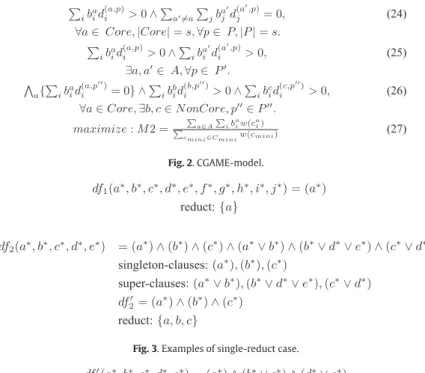
Fig. 2. CGAME-model.
Fig. 3. Examples of single-reduct case.
Fig. 4. An example of the multiple-reducts case.
Assigning thebaisto values such that the objective function (27) reaches a maximum is equivalent to computing a C-GAME set of cuts. Branch and bound optimisation algorithms (B&B) can be used to solve CGAME-Model.
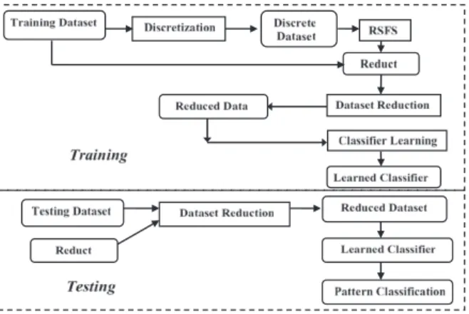
3.5. Elimination of the single-reduct case
Each clause within the original unsimplified discernibility functiondfis associated with a pairpwithin the discernibility table
A
∗such that each attribute of the clause discerns that pair. Constraint (25) states that both attributesaandadiscern a pairp, so(
a∗∨
a∗)
becomes a clause ofdf, wherea∗anda∗are Boolean variables corresponding toaanda. Ifaand/ora arecoreattributes,(
a∗∨
a∗)
would be removed duringdfsimplification, because(
a∗∨
a∗)
is a super-clause3 of botha∗ anda∗.There are 2 forms of unsimplified discernibility functiondfwhich lead to a single reduct within the dataset. The first form ofdfis where thedfconsists only of singleton-clauses.4 In this case, the reduct consists of the attributes which correspond to the Boolean variables of the singleton-clauses. An example of the first form isdf1(Fig.3). The second form ofdfis where dfconsists of singleton-clauses and super-clauses of the singleton-clauses.df2(Fig.3) is an example of the second form. For the second form, all the super-clauses of singleton-clauses are removed fromdfduringdfsimplification. The simplified discernibility functiondfwill contain only the singleton-clauses, so one reduct would be present in the dataset.
If, however,dfdoes not include super-clauses of any singleton-clauses, there would be multiple reducts in the dataset. An example is shown in Fig.4, wheredf3is a simplified discernibility function.df3does not contain super-clauses of
(
a∗)
and there are four reducts within the dataset.Coresize is relatively small compared to the dataset dimensionality. However, usingcoreas a feature subset could remove too much information from the original dataset such that, consequently, the classification performance may be poor, hence the presence of multiple reducts is often to be preferred to the presence of only one reduct. In order to eliminate the single-reduct case in the discrete dataset, constraint (26) is enforced to create non-singleton clauses which are not super-clauses of the singleton-clauses withindf.3.6. The C-GAME discretization algorithm
The C-GAME discretization algorithm repeatedly computes a C-GAME set of cuts by solving CGAME-Model and evaluates the performance of the set of cuts based on the accuracy of the reducts found by a genetic algorithm (GA) [4]. When the newly found set of cuts satisfies the condition that most of the GA-found reducts outperform C4.5’s accuracy, the discretization process stops (Fig.5). The GA employed by the C-GAME algorithm is presented in AppendixAppendix B. The
3 A super-clause of a clause includes that clause, e.g.(b∗∨c∗)is a super-clause of both(b∗)and(c∗). 4
Fig. 5. Pseudo-code of the C-GAME discretization algorithm.
C-GAME algorithm can be applied to both consistent and inconsistent decision tables. Discernibility tables of inconsistent decision tables are computed in the same way that the discernibility tables of consistent decision tables are computed. After computing the discernibility tables, they are input to C-GAME together with the training and testing5 datasets to obtain a discrete training dataset. AppendixAppendix Cpresents 2 example runs of the C-GAME algorithm: one for a consistent decision table, the other for an inconsistent decision table.
4. Performance evaluation
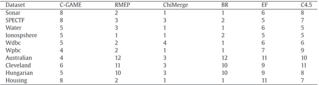
The performance of C-GAME is evaluated as a pre-processor for RSFS. C-GAME is integrated with Johnson’s algorithm and four classification algorithms: C4.5 [16] decision tree learning algorithm, multi-layer perceptrons, radial basis function networks and the K-nearest neighbour method using the framework in Fig.6. Johnson’s algorithm (AppendixAppendix B) finds a smallest reduct and is used for RSFS. C-GAME integration6 is compared with RMEP integration,7Chimerge integra-tion8, Boolean Reasoning integration9 and Equal Frequency integration10 using 10 datasets (Table8) chosen from the UCI Machine Learning Repository [15]. The SPECTF, Water, Ionosphere and Wdbc datasets have been split into the training and testing datasets as suggested by their providers; the remaining six datasets has been split into 2/3 training and 1/3 testing datasets, respectively.
4.1. Decision trees
C-GAME integration outperforms C4.5 for each of the 10 chosen datasets (Table9). C-GAME integration outperforms the other four discretization integrations for the majority of the ten datasets (Table9). For most of the 10 datasets, the other four discretization integrations have lower accuracy than C4.5 (Table9). The results show that generating cores during discretization using C-GAME should lead to a higher accuracy than that obtained with C4.5.
4.2. Multi-layer perceptrons
For each of the 10 datasets, a multi-layer perceptron (MLP) network with 2 hidden layers of 10 nodes and two output nodes is applied instead of C4.5. For eight datasets, C-GAME outperforms the MLPs (Table10). For the remaining two datasets,
5
Evaluating a C-GAME set of cuts using the testing dataset gives a good measure of its performance, because the testing dataset is independent of the training dataset.
6 C-GAME integration is the integrated classification approach made up of C-GAME, Johnson’s algorithm and a classification algorithm. 7 RMEP integration is the integrated classification approach made up of RMEP, Johnson’s algorithm and a classification algorithm. 8
Chimerge integration is the integrated classification approach made up of Chimerge, Johnson’s algorithm and a classification algorithm.
9 Boolean Reasoning integration is the integrated classification approach made up of Boolean Reasoning, Johnson’s algorithm and a classification algorithm. 10
Fig. 6. Integrated RSFS classification framework. Table 8
Datasets description.
Datasets Attributes Train Test Classes
1. Sonar 60 139 69 2 2. SPECTF 44 80 269 2 3. Water 38 260 261 2 4. Ionosphere 34 105 246 2 5. Wdbc 30 190 379 2 6. Wpbc 33 129 65 2 7. Australian 14 460 230 2 8. Cleveland 13 202 101 2 9. Hungarian 13 196 98 2 10. Housing 13 338 168 2 Table 9
Classification accuracy with C4.5.
Data sets C-GAME C4.5 RMEP BR Chimerge EF
Sonar 87 84.1 50.7 72.5 72.5 84.1 SPECTF 81 77.3 20.4 20.4 51.7 20.4 Water 98.9 98.1 96.9 97.3 97.3 97.3 Ionosphere 91.1 81.7 82.9 76.8 82.9 87.8 Wdbc 92.6 91.3 69.1 69.1 88.1 69.1 Wpbc 73.8 64.6 73.8 73.8 73.8 63.1 Australian 83 82.6 83.9 84.3 59.6 83.9 Cleveland 77.2 76.2 78.2 77.2 69.3 73.3 Hungarian 85.7 79.6 79.2 85.7 68.4 77.6 Housing 83.3 82.1 65.2 83.3 65.5 82.7 Table 10
Classification accuracy with MLPs.
Data sets C-GAME MLP RMEP BR Chimerge EF
Sonar 89.9 88.4 55.1 71 71 73.9 Spectf 76.6 75.1 34.6 45.4 34.2 69.9 Water 98.5 98 79.3 97.3 97.3 97.3 Ionosphere 88.6 88.2 60.6 60.6 88.2 86.6 Wdbc 14.5 5.8 11.6 11.6 11.6 7.9 Wpbc 81.5 80 73.8 73.8 73.8 73.8 Australian 85.2 83.9 82.2 63.9 83.9 82.6 Cleveland 80.2 80.2 80.2 75.2 80.2 75.2 Hungarian 86.7 80.6 83.6 84.7 84.7 84.7 Housing 81.5 81.5 64.9 81 62.5 81.5
C-GAME has the same accuracy as the MLPs. C-GAME outperforms the other four discretization methods for most of the 10 datasets. The other four discretization methods have lower accuracy than the MLPs for the majority of the 10 datasets (Table 10). The results show that generating cores during discretization should lead to a higher accuracy than that obtained with the MLPs.
4.3. RBF networks
Radial basis functions (RBF) networks have also been analysed. For nine datasets, C-GAME outperforms RBF networks (Table11). For the remaining dataset, C-GAME has the same accuracy as RBF networks. C-GAME outperforms the other four
Table 11
Classification accuracy with RBF networks.
Data sets C-GAME RBF RMEP BR Chimerge EF
Sonar 79.7 75.4 55.1 71 71 73.9 Spectf 77 75.1 46.8 58.7 64.3 69.9 Water 98.9 98.1 97.3 97.3 97.3 97.3 Ionosphere 88.6 88.2 60.6 60.6 88.2 86.6 Wdbc 13.7 5.8 7.6 11.6 11.6 7.9 Wpbc 84.6 80 73.8 73.8 73.8 73.8 Australian 85.2 83.9 82.1 63.9 83.9 82.6 Cleveland 80.2 80.2 80.2 75.2 80.2 75.2 Hungarian 86.7 80.6 83.6 84.7 84.7 84.7 Housing 75 73.8 64.3 62.5 70.8 70.8 Table 12
Classification accuracy with K-NN.
Data sets C-GAME K-NN RMEP BR Chimerge EF
Sonar 82.6 76.8 59.4 66.7 66.7 82.6 Spectf 68.8 60.6 62.1 59.5 61.3 68.8 Water 97.3 97.3 97.3 97.3 97.3 97.3 Ionosphere 89.4 87.8 72 72 84.6 87.8 Wdbc 17.4 4.2 13.7 13.7 13.7 9.8 Wpbc 75.4 67.7 66.2 69.2 70.8 70.8 Australian 86.5 84.8 87 65.2 85.7 84.8 Cleveland 75.2 75.2 74.3 74.3 78.2 73.3 Hungarian 89.8 89.8 89.8 84.7 82.7 82.7 Housing 85.7 85.7 64.9 81 66.1 85.7 Table 13
Comparison of average sizes of reducts.
C-GAME RMEP ChiMerge BR EF C4.5
5.7 4.8 2.1 3.9 7.5 7.6
discretization methods for the majority of the 10 datasets. The other four discretization methods have lower accuracy than RBF networks for the majority of the 10 datasets (Table11). The results show that generating cores during discretization using C-GAME should lead to a higher accuracy than that obtained with the RBF networks.
4.4. K-nearest neighbours
K-nearest neighbours classification (K-NN) is also used instead of C4.5. For seven datasets, C-GAME leads to a higher accuracy than that obtained from K-NN (K = 5) (Table12). For the remaining three datasets, C-GAME has the same accuracy as K-NN. C-GAME outperforms the other four discretization methods for most of the 10 datasets. The other four discretization methods have a lower accuracy than that obtained with K-NN for most of the datasets (Table12). The results show that generating cores during discretization using C-GAME should lead to a higher accuracy than that obtained with the K-NN classifier.
4.5. Reducts sizes
C-GAME, RMEP, ChiMerge, Boolean Reasoning (BR) and Equal Frequency (EF) result in different reducts sizes. C4.5 selects features during decision tree learning. The features selected by C4.5 form a reduct. For each method, including C4.5, the average reduct size over the ten datasets is computed as follows:
Saverage
=
i∈D sizei|
D|
,
(28)whereDis a set of datasets;sizeiis the reduct size of dataseti. The average reduct size of each of the methods is illustrated in Table13. C4.5 leads to the largest average reduct size among the six methods. Chimerge leads to the smallest average reduct size among the methods. C-GAME leads to a medium average reduct size among the methods. For the six high dimensional datasets - Sonar, SPECTF, Water, Ionosphere, Wdbc and Wpbc - C-GAME and C4.5 obtain the largest or the 2nd largest reduct sizes among the six methods (Table14). For the Australian, Cleveland and Hungerian datasets, C-GAME leads to the 2nd smallest reduct size among the methods. For these three datasets, C4.5 is in the top three largest reduct sizes obtained. For the Housing dataset, C-GAME leads to the 2nd largest reduct size and C4.5 leads to the 3rd largest reduct size.
Table 14 Reducts sizes.
Dataset C-GAME RMEP ChiMerge BR EF C4.5
Sonar 8 2 1 1 6 8 SPECTF 8 3 3 2 5 7 Water 5 3 1 1 6 5 Ionospshere 5 1 1 2 5 5 Wdbc 5 2 4 1 6 6 Wpbc 4 2 1 1 7 9 Australian 4 12 3 12 11 10 Cleveland 6 11 3 10 9 11 Hungarian 5 10 3 10 9 8 Housing 8 2 1 1 11 7
4.6. Total number of reducts
4.6.1. An upper bound on the total number of reducts
Letdfbe the simplified discernibility function of a decision table
A
=
(
U,
A∪{
d}
)
anddfcontainskclausesa∗∈ci∗a∗ : df=
k i=1 ⎛ ⎜ ⎝ a∗∈c∗i a∗ ⎞ ⎟ ⎠,
(29)whereci∗
= {
a∗|∃
a∈
A}
. LetMbe a collection of feature subsets which correspond to the clauses withindfsuch that M=
Si|S
i= {a|a
∈
A∧
a∗∈
c∗i∧
1≤
i≤
k}
,
(30)wherea∗is a Boolean variable corresponding toa;kis the cardinality ofM. An orderedk-tuple [27] is
(
s1,
s2, . . . ,
sk)
where si∈
Si, 1≤
i≤
k. Eachk-tuple corresponds to a minimal hitting set ofMbecause for eachS∈
M, a minimal hitting set includes exactly one attributes∈
S. The set of all thek-tuples iski=1Si= {
(
a1,
a2, . . . ,
ak)
|
ai∈
Si,
1≤
i≤
k}
. LetTk denoteki=1Si.Tkalso contains thosek-tuples which correspond to the same minimal hitting set. For example, let a simplified discernibility functiondfbedf=
(
a∗∨
b∗∨
c∗∨
g∗)
∧
(
a∗∨
b∗∨
c∗∨
d∗∨e
∗)
∧
(
f∗)
.M= {{a
,
b,
c,
g},
{a
,
b,
c,
d,
e},
{f
}}
. The cardinality ofMis 3. The ordered 3-tuples and the corresponding minimal hitting sets are as follows:(
a,
a,
f)
→ {
a,
f}
, (
a,
b,
f)
→ {
a,
b,
f}
, (
a,
d,
f)
→ {
a,
d,
f}
, (
a,
e,
f)
→ {
a,
e,
f}
,
(
a,
c,
f)
→ {
a,
c,
f}
, (
b,
a,
f)
→ {
a,
b,
f}
, (
b,
b,
f)
→ {
b,
f}
, (
b,
d,
f)
→ {
b,
d,
f}
,
(
b,
e,
f)
→ {
b,
e,
f}
, (
b,
c,
f)
→ {
b,
c,
f}
, (
c,
a,
f)
→ {
a,
c,
f}
, (
c,
b,
f)
→ {
b,
c,
f}
,
(
c,
d,
f)
→ {
c,
d,
f}
, (
c,
e,
f)
→ {
c,
e,
f}
, (
c,
c,
f)
→ {
c,
f}
, (
g,
a,
f)
→ {
a,
f,
g}
,
(
g,
b,
f)
→ {
b,
g,
f}
, (
g,
d,
f)
→ {
d,
f,
g}
, (
g,
e,
f)
→ {
e,
f,
g}
, (
g,
c,
f)
→ {
c,
f,
g}
,
where
→
denotes ‘corresponds to’. Both(
a,
b,
f)
and(
b,
a,
f)
correspond to{
a,
b,
f}
; both(
b,
c,
f)
and(
c,
b,
f)
correspond to{
b,
c,
f}
; both(
a,
c,
f)
and(
c,
a,
f)
correspond to{
a,
c,
f}
. The total number of minimal hitting sets is 17.3i=1|
Si| =
20 whereSi∈
Mandi=
1,
2,
3. Therefore, an upper bound on the total number of minimal hitting sets (reducts) of the decision tableA
is|
Tk| =
ki=1|
Si|
.4.6.2. Effect of discretization on the total number of reducts
The five discretization approaches result in different total numbers of reducts in the discrete datasets. For the datasets Sonar, Spectf, Water, Ionosphere, Wdbc and Wpbc which have dimensionalities between 30 and 60, C-GAME results in fewer reducts within the discrete datasets than the other four approaches. This is because the upper bounds of the total numbers of reducts from the C-GAME-discrete11datasets are smaller than the upper bounds of the total numbers of reducts corresponding to the discrete datasets that are output by the other four methods (Table15), where ‘+Inf’ is any number larger than the largest number12 that can be represented by the IEEE 754 floatingpoint standard. For the remaining datasets -Australian, Cleveland, Hungerian and Housing - which contain either 13 or 14 attributes, the RMEP, Boolean Reasoning and Equal frequency methods result in fewer reducts than does C-GAME (Table15). For these four datasets C-GAME results in fewer reducts than does Chimerge.
11A C-GAME-discrete dataset is the discrete dataset that C-GAME outputs. 12
Table 15
Upper bounds on total numbers of reducts.
Datasets Attributes C-GAME RMEP ChiMerge BR EF
Sonar 60 3.13×1041 +Inf 1.57×1097 +Inf +Inf
SPECTF 44 6.05×10⁷ +Inf +Inf +Inf +Inf
Water 38 4004 3.95×10273 6.79×10178 +Inf +Inf
Ionospshere 34 11 6.84×10171 6×1091 +Inf +Inf
Wdbc 30 9177 1.54×1063 3.32×1042 2.68×1063 +Inf Wpbc 33 9.66×1045 3.7×1076 7.9×1026 9.55×1074 +Inf Australian 14 13,063,680 1 8.33×1036 2 192 Cleveland 13 5.13×10¹⁵ 1 5.48×1039 2 27,648 Hungarian 13 2 1 259,200 6 1 Housing 13 4 2 1,296,000 5184 32
Sonar0 Spectf Water Ionosphere Wdbc Wpbc Australian Cleveland Hungarian Housing
200 400 600 800 1000 1200 1400 1600 1800 2000 datasets generations of GA C−GAME RMEP ChiMerge Boolean Equal Frequency
Fig. 7. Speed comparison of GA.
4.7. Speed of RSFS algorithms
Johnson’s algorithm and the GA [4] are used to find reducts. To measure the speed of the GA, the number of generations before convergence is counted. For Johnson’s algorithm, the number of times that thewhileloop body is executed is counted. 4.7.1. Speed of genetic algorithm
For the datasets Sonar, SPECTF, Water, Ionosphere, Wdbc, Wpbc, the GA converges significantly faster on the six C-GAME discrete datasets than it converges on the discrete datasets output by the other four discretization methods (Fig. 7). This is because the C-GAME-discrete datasets contain fewer reducts than the other discrete datasets (Table15), so the GA searches fewer candidate reducts in order to find the smallest reducts. Moreover, the GA converges most quickly on Boolean-Reasoning-discrete Australian, Boolean-Reasoning-discrete Cleveland, C-GAME-discrete Hungarian, RMEP-discrete Hungarian, Boolean-Reasoning-discrete Hungarian, Equal-Fequency-discrete Hungarian, C-GAME-discrete Housing and RMEP-discrete Housing datasets (Fig.7). These discrete datasets contain very few reducts (Table15). The GA converges most slowly on the EF-discrete Ionosphere dataset.
4.7.2. Speed of Johnson’s algorithm
For each of the 10 datasets, if its core size is greater than 0, there is a strong correlation (0.93) between the core size and the speed of Johnson’s algorithm for that dataset, where algorithm speed is measured by the number of executions of the loop body (Tables16and17). If the core size equals 0, then there appears to be no correlation between the core size and the speed of Johnson’s algorithm (Tables16and17). Therefore, if core size iskwherek
>
0, the speed of Johnson’s algorithm is at leastk.Table 16
Speed of Johnson’s algorithm and core size.
Datasets C-GAME RMEP Chimerge
Core size Johnson Core size Johnson Core size Johnson
Sonar 7 8 0 2 0 1 Spectf 7 8 0 3 0 3 Water 4 5 0 3 0 1 Ionosphere 4 5 0 1 0 1 Wdbc 4 5 0 2 0 4 Wpbc 3 4 0 2 0 1 Australian 3 4 12 12 0 3 Cleveland 4 6 11 11 0 3 Hungarian 4 5 10 10 0 3 Housing 7 8 1 2 0 1 Table 17
Speed of Johnson’s algorithm and core size.
Datasets BR EF
Core size Johnson Core size Johnson
Sonar 0 1 0 6 Spectf 0 2 0 5 Water 0 1 0 6 Ionosphere 0 2 0 5 Wdbc 0 1 0 6 Wpbc 0 1 0 7 Australian 11 12 8 11 Cleveland 9 10 4 9 Hungarian 7 10 9 9 Housing 0 1 9 11 5. Conclusion
This work has demonstrated that C-GAME discretization is a promising pre-processing method for RSFS in pattern classi-fication. C-GAME integration outperforms C4.5 on each of the 10 UCI datasets that have been analysed and outperforms MLPs, RBF networks and K-NN classification approaches on most of these datasets. C-GAME also outperforms RMEP, Chimerge, Boolean Reasoning and Equal frequency as a pre-processor of RSFS on most of these datasets. For high dimensional datasets, C-GAME discretization may lead to a smaller total number of reducts within the discrete datasets compared with the other four discretization methods. C-GAME may also lead to faster convergence speed of genetic algorithms than the other four discretization methods. If the total number of reducts within a dataset affects the speed of a given RSFS algorithm, such that the fewer the number of reducts within a dataset, the faster the speed of that RSFS algorithm, then C-GAME could also result in a faster speed for the RSFS algorithm than the other four discretization methods. In terms of dimensionality reduction, C-GAME leads to a medium dimensionality reduction effect compared with the other four discretization methods and C4.5. Higher dimensional datasets such as text datasets, computer networks intrusion datasets and micro array gene expression datasets could be used to further evaluate the C-GAME peformance. As discretization methods can also be applied to Bayesian learning and association rules mining approaches as pre-processors, C-GAME could be used in such approaches to evaluate performance.
Appendix A. Constraint satisfaction problems
A constraint satisfaction problem (CSP) consists of a finite set of variables, each of which is associated with a finite domain and a set of constraints that restricts the values the variables can simultaneously take [17]. The domain of a variable is a set of all the possible values that can be assigned to the variable. A label is a variable-value pair, denoting the assignment of a value to a variable. A compound label is a set of labels over some of the variables. A constraint can be viewed as a set of compound labels over some or all of the variables. A total assignment is a compound label on all the variables of a CSP. A solution to a CSP is a total assignment satisfying all the constraints simultaneously. The search space of a CSP is the set of all the possible total assignments [18]. The size of the search space is the number of all the possible total assignments [18,17]:x∈ZDx, where Zis the set of all variables, andDxis the domain ofx. A CSP can be reduced to an equivalent but simpler CSP by removing redundant values from the domains and removing redundant compound labels from the constraints in the original CSP [17]. This process is calledconstraint propagation. No solutions exist if the domain of any variable or any constraint is reduced to an empty set [17]. A CSP can be represented as a type of graph termed a constraint graph [17]. Constraint propagation maintains the consistencies of the constraint graph of the CSP. A constraint satisfaction optimization problem (CSOP) is a CSP with an objective function. The solution to the CSOP is the total assignment satisfying all the constraints simultaneously whilst maximizing or minimizing the objective function. CSOPs are solved using optimization algorithms such as branch and bound [17].
Fig. 8. Pseudo-code for the genetic algorithm.
Fig. 9. Pseudo-code for Johnson’s algorithm.
Appendix B. Reducts computation
A subset of attributes is a hitting set of the df, if it has a non-empty intersection with each clause of the df. It is a minimal hitting set if it is no longer a hitting set when any of its elements is removed. Reducts can be computed as minimal hitting sets of the df using a genetic algorithm (GA) proposed in [4]. The hitting fraction of a subset is the ratio of the number of non-empty intersections of the subset with the discernibility function to its cardinality [4]:
h
(
B)
=
|{S
∈
D|S∩
B= ∅}|
|
D|
,
(31)whereBis a subset,h
(
B)
is the hitting fraction ofB,Dis a discernibility function. A subset is a minimal hitting set if its hitting fraction is equal to 1 and has a minimal size. For finding minimal hitting sets, the fitness function of the GA is defined as [4]:f
(
B)
=
|
A| − |
B|
|
A|
+
h(
B),
(32)whereAis the set of all condition attributes andBis a chromosome. The GA pseudo code is illustrated in Fig.8[4], where P denotes a population and Parents[i] denotes a set of selected individuals to undergo a genetic operation, so Parents[1..3] corresponds to three sets of selected individuals and Offspring[i] denotes the resulting set of offspring. The stop criterion of the GA is that there is no improvement in the average fitness of the current population over a predefined number of generations (iterations). Johnson’s algorithm [5] is a greedy heuristic which finds a single reduct of minimal length. The algorithm iteratively selects the attribute that is present in the most clauses remaining in the df and remove those clauses from the df. The algorithm stops when all clauses have been removed from the df (Fig.9).
Appendix C. Example runs of C-GAME discretization algorithm
Appendix C.1. A consistent decision table
The continuous decision table DT (Table18) is consistent. Its simplified discernibility functiondfisdf
=
(
a∗∨
b∗∨
d∗∨
e∗)
∧
(
a∗∨
c∗∨
d∗∨
e∗)
∧
(
b∗∨
c∗∨
d∗∨
e∗∨
f∗)
andcoreof DT is empty. When the C-GAME algorithm is applied to DT, the C-GAME-discrete decision table DT’ contains a non-emptycore:{a
,
b}and is also consistent (Table19). The simplified discernibility functiondfof DT’ isdf=
(
a∗)
∧
(
b∗)
∧
(
c∗∨
d∗)
∧
(
e∗∨
f∗)
.Coreof DT’ is{
a,
b}
.Table 18
DT: an consistent decision table.
U a b c d e f Class o1 58 150 283 162 1 3 0 o2 54 124 266 109 2.2 7 1 o3 51 130 305 142 1.2 7 1 o4 54 120 188 113 1.4 7 1 o5 60 125 258 141 2.8 7 1 o6 44 108 141 175 0.6 3 0 o7 49 120 188 139 2 7 1 o8 57 128 229 150 0.4 7 1 o9 41 135 203 132 0 6 0 o10 35 120 198 130 1.6 7 1 o11 51 125 245 166 2.4 3 0 o12 41 112 250 179 0 3 0 o13 67 100 299 125 0.9 3 1 o14 58 128 259 130 3 7 1 o15 63 108 269 169 1.8 3 1 o16 34 118 210 192 0.7 3 0 o17 66 112 212 132 0.1 3 0 o18 30 98 212 122 1.6 3 1 o19 46 120 249 144 0.8 7 1 o20 42 91 236 124 0.52 2 0 Table 19
DT’: the consistent discrete decision table.
U a b c d e f Class o1 4 8 6 2 2 0 0 o2 4 4 5 0 3 1 1 o3 4 7 7 2 2 1 1 o4 4 3 1 1 2 1 1 o5 4 5 5 2 6 1 1 o6 4 2 0 3 2 0 0 o7 4 3 1 2 3 1 1 o8 4 6 5 2 1 1 1 o9 3 8 3 2 0 1 0 o10 2 3 2 2 2 1 1 o11 4 5 5 2 4 0 0 o12 3 3 5 4 0 0 0 o13 4 1 7 2 2 0 1 o14 4 6 5 2 6 1 1 o15 4 2 5 2 2 0 1 o16 1 3 4 4 2 0 0 o17 4 3 5 2 0 0 0 o18 0 0 5 2 2 0 1 o19 4 3 5 2 2 1 1 o20 4 0 5 2 2 0 0 Table 20
DT2: an inconsistent decision table.
U a b c d e f Class o1 58 150 283 162 1 3 0 o2 54 124 266 109 2.2 7 1 o3 51 130 305 142 1.2 7 1 o4 54 120 188 113 1.4 7 1 o5 60 125 258 141 2.8 7 1 o6 44 108 141 175 0.6 3 0 o7 49 120 188 139 2 7 1 o8 57 128 229 150 0.4 7 1 o9 41 135 203 132 0 6 0 o10 35 120 198 130 1.6 7 1 o11 51 125 245 166 2.4 3 0 o12 41 112 250 179 0 3 0 o13 67 100 299 125 0.9 3 1 o14 58 128 259 130 3 7 1 o15 63 108 269 169 1.8 3 1 o16 34 118 210 192 0.7 3 0 o17 66 112 212 132 0.1 3 0 o18 66 112 212 132 0.1 3 1 o19 46 120 249 144 0.8 7 1 o20 46 120 249 144 0.8 7 0
Table 21
DT2’: the inconsistent discrete decision table.
U a b c d e f Class o1 2 6 8 5 1 0 0 o2 1 4 6 0 1 1 1 o3 1 5 9 3 1 1 1 o4 1 4 1 1 1 1 1 o5 2 4 5 3 1 1 1 o6 1 1 0 8 1 0 0 o7 1 4 1 3 1 1 1 o8 1 4 5 4 1 1 1 o9 1 6 3 3 0 1 0 o10 1 4 2 3 1 1 1 o11 1 4 5 6 1 0 0 o12 1 2 5 9 0 0 0 o13 2 0 9 2 1 0 1 o14 2 4 5 3 1 1 1 o15 2 1 7 7 1 0 1 o16 0 3 4 9 1 0 0 o17 2 2 5 3 0 0 0 o18 2 2 5 3 0 0 1 o19 1 4 5 3 1 1 1 o20 1 4 5 3 1 1 0
Appendix C.2. An inconsistent decision table
The continuous decision table DT2 (Table20) is inconsistent, because objectso17ando18belong to different classes and have identical attributes values and this is also true for objectso19ando20. The simplified discernibility functiondf2 of DT2 isdf2
=
(
a∗∨
c∗∨
d∗∨
e∗)
∧
(
a∗∨
b∗∨
c∗∨
e∗∨
f∗)
∧
(
b∗∨
c∗∨
d∗∨
e∗∨
f∗)
andcoreof DT2 is empty. When the C-GAME algorithm is applied to DT2, the C-GAME-discrete decision table DT2’ (Table21) is also inconsistent. The simplified discernibilitydf2of DT2’ isdf2=
(
c∗)
∧
(
d∗)
∧
(
a∗)
∧
(
b∗∨
e∗∨
f∗)
.Coreof DT2’ is{
a,
c,
d}
.References
[1] L. Polkowski, Rough Sets. Mathematical Foundations, Physica-Verlag, Berlin, 2002. [2] C.M. Bishop, Neural Networks for Pattern Recognition, Oxford University Press, 1995.
[3] R. Jensen, Q. Shen, Semantics-preserving dimensionality reduction: rough and fuzzy-rough-based approaches, IEEE Transactions on Knowledge and Data Engineering 16 (12) (2004) 1457–1472.
[4] S. Vinterbo, A. Ohrn, Minimal approximate hitting sets and rule templates, International Journal of Approximate Reasoning 25 (2) (2000) 123–143. [5] D.S. Johnson, Approximation algorithms for combinatorial problems, Journal of Computer and System Sciences 9 (1974) 256–278.
[6] M. Goodarzi, M.P. Freitas, R. Jensen, Feature selection and linear/nonlinear regression methods for the accurate prediction of glycogen synthase Kinase-3B inhibitory activities, Journal of Chemical Information and Modeling 49 (4) (2009) 824832.
[7] X. Wang, J. Yang, X. Teng, W. Xia, R. Jensen, Feature selection based on rough sets and particle swarm optimization, Pattern Recognition Letters 28 (4) (2007) 459–471.
[8] Z. Pawlak, Rough Sets: Theoretical Aspects of Reasoning about Data, Kluwer Academic Publishers, 1991.
[9] R.W. Swiniarski, A. Skowron, Rough set methods in feature selection and recognition, Pattern Recognition Letters 24 (2003) 833–849.
[10] H. Ming, A rough set based hybrid method to feature selection, in: International Symposium on Knowledge Acquisition and Modeling, 2008, pp. 585–588. [11] A. An, Y. Huang, X. Huang, N. Cercone, Feature selection with rough sets for web page classification, Transactions on Rough Sets 2 (2004) 1–13. [12] R.W. Swiniarski, A. Skowron, Rough set methods in feature selection and recognition, Pattern Recognition Letters 24 (2003) 833–849.
[13] J. Dougherty, R. Kohavi, M. Sahami, Supervised and unsupervised discretization of continuous features, in: Proceedings of the Twelfth International Conference on Machine Learning, 1995, pp. 194–202.
[14] H.N. Son, Discretization of real value attributes: a Boolean reasoning approach, Ph.D. Thesis, Department of Computer Science, Warsaw University, 1997. [15] S. Hettich, L.C. Blake, J.C. Merz, UCI Repository of machine learning databases,http://www.ics.uci.edu/∼mlearn/MLRepository.html, University of California,
Irvine, Department of Information and Computer Sciences, 1998.
[16] R.J. Quinlan, C4.5: Programs for Machine Learning, Morgan Kaufman, San Mateo, CA, 1993.
[17] E.P.K. Tsang, Foundations of Constraint Satisfaction, Academic Press Limited, London and San Diego, 1993.
[18] A.M. Cheadle, W. Harvey, A.J. Sadler, J. Schimpf, K. Shen, M. G. Wallace, ECliPSe: a tutorial introduction, 2009. Available from:http://www.eclipse-clp.org/
[19] S.H. Nguyen, A. Skrowron, Quantization of real values attributes, Rough set and Boolean reasoning approach, in: Proceedings of the Second Joint Annual Conference on Information Sciences, Wrightsville Beach, North Carolina, 1995, pp. 34–37.
[20] R.M. Chmielewski, W.J. Grzymala-Busse, Global discretization of continuous attributes as preprocessing for machine learning, International Journal of Approximate Reasoning 15 (1996) 319–331.
[21] J. Gama, L. Torgo, C. Soares, Dynamic discretization of continuous attributes, Progress in artificial intelligence - IBERAMIA 98, Lecture Notes in Computer Science, vol. 1484, Springer, 1998, pp. 160–169.
[22] H. Liu, F. Hussain, C.L. Tan, M. Dash, Discretization: an enabling technique, Data Mining and Knowledge Discovery, vol. 6(4), Kluwer Academic Publishers, 2002, pp. 393–423.
[23] I.H. Witten, E. Frank, Data Mining: Practical Machine Learning Tools and Techniques, second ed., Morgan Kaufman, 2005. [24] D. Hand, H. Mannila, P. Smyth, Principles of Data Mining, MIT Press, 2001.
[25] J. Han, M. Kamber, Data Mining: Concepts and Techniques, Academic Press, 2000.
[26] K. Cios, W. Pedrycz, R. Swiniarski, Data Mining Methods for Knowledge Discovery, Kluwer Academic Publishers, 1998. [27] B. Kolman, R.C. Busby, S.C. Ross, Discrete Mathematical Structures, fourth ed., Higher Education Press, Pearson Education, 2001. [28] I. Guyon, A. Elisseeff, An introduction to variable and feature selection, Journal of Machine Learning Research 3 (2003) 1157–1182.
[29] D. Tian, J. Keane, X. Zeng, Core-generating approximate minimum entropy discretization for rough set feature selection: an experimental investigation, in: Proceedings of the 16th IEEE International Conference on Fuzzy Systems, Imperial College, London, UK, 2007.
[30] E. Tsang, D. Chen, D.S. Yeung, Approximations and reducts with covering generalized rough sets, Computers and Mathematics with Applications 56 (2008) 279–289.
[31] D. Yamaguchi, Attribute dependency functions considering data efficiency, International Journal of Approximate Reasoning 51 (1) (2009) 89–98. [32] T. Yang, Q. Li, Reduction about approximation spaces of covering generalized rough sets, International Journal of Approximate Reasoning 51 (3) (2010)
335–345.
[33] Q. Hu, L. Zhang, D. Cheng, W. Pedrycz, D. Yu, Gaussian Kernel based fuzzy rough sets: models, uncertainty measures and applications, International Journal of Approximate Reasoning 51 (4) (2010) 453–471.
[34] N.J. Pizzi, W. Pedrycz, Aggregating multiple classification results using fuzzy integration and stochastic feature selection, International Journal of Approxi-mate Reasoning 51 (8) (2010) 883–894.
[35] M.M. Drugan, M.A. Wiering, Feature selection for Bayesian network classifiers using the MDL-FS score, International Journal of Approximate Reasoning 51 (6) (2010) 695–717.
[36] L. Sanchez, M.R. Suarez, J.R. Villar, I. Couso, Mutual information-based feature selection and partition design in fuzzy rule-based classifiers from vague data, International Journal of Approximate Reasoning 49 (3) (2008) 607–622.