SIMULATION OF TRAIN CONTROL SYSTEMS IN THREE DIMENSIONAL
ENVIRONMENT
B. Vincze 1, G. Tarnai 2 1
Budapest University of Technology and Economics, Dept. of Control and Transport and Automation Address: Bertalan L. u. 2., Budapest, Hungary H-1111
Phone: : (+36-1) 463-1044 Fax (+36-1) 463-3087, e-mail:[email protected] web:web.axelero.hu/egzo
2
Budapest University of Technology and Economics, Dept. of Control and Transport and Automation Address: Bertalan L. u. 2., Budapest, Hungary H-1111
Phone: (+36-1) 463-1990 Fax (+36-1) 463-3087, e-mail: [email protected]
Abstract: This paper describes a complex, all-in-one simulation tool with some application examples. The system can be efficiently used for simulating all kind of train control systems in a three dimensional environ-ment.
Keywords: Simulation, Train Control, ETCS, 3D
1 INTRODUCTION
As the new ERTMS/ETCS system spreads through Europe with new technologies in railway operation, there is a huge demand for new, inno-vative solutions for making the design and train-ing processes of train control systems faster, more accurate and more efficient.
The application of such state of the art technologies, like GSM-R for safety communica-tion in train control systems and GPS/Galileo for train positioning (especially for lines with low traffic density) requires new techniques or even new approach in simulation and CAD systems.
The appearance of new hardware and soft-ware technologies in the past decade made possi-ble to create more complex, realistic but also computing-intensive simulation methods in the transport industry.
Nowadays, many railway companies in Europe use simulators with 3D views for driver training/demonstration purposes (e.g. DB-ICE Simulator, developed by DB Forschungs und Technologiezentrum, München).
Moreover, complex simulations are devel-oped by RENFE within the framework of the HUSARE project, which aims to establish a common method for evaluating and improving human management in order to increase safety and reliability for European cross-border opera-tions.
During our research activity, a design and a real-time simulation tool have been developed,
which is characterized by a fully modular archi-tecture (Vincze et al, 2004). This architecture
was designed to fulfil all needs related to train control system design and testing, in a three dimensional environment.
Most simulation tools (Terada, N.; 2004, K. Lano et al, 2004.) take advantage of the fact that
trains can move only forwards or backwards, so that the position can be represented with a single distance coordinate and a track section identifier. There are so-called “quasi-3D” simulation tools, commonly used for train driver training. These tools usually have cab view, which is generated from pre-recorded video sequences (e.g. V63 simulator of the Hungarian Railway Museum).
Unlike these systems, our developed tools are fully three dimensional. It means that each object has a spatial position and orientation.
The three dimensional approach makes pos-sible to create accurate dynamic models, to test new technologies like GPS/GSM-R, or to per-form realistic test runs. Thus, the tool can be efficiently used not just for planning, but e.g. for training locomotive drivers or for demonstrating the operation of various railway safety equip-ments.
2 THE SIMULATION STRUCTURE
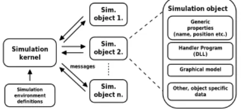
The simulation tool is object oriented. Each object resides in a separate dynamic link library, which means that any programming language can
be used for creating objects. This allows great flexibility, and makes possible to add, modify or remove objects without touching the system kernel (Fig.1.)
Each object can have a handler program, a three-dimensional graphical model, name, type, priority, position, mass, orientation and other object specific data. For flexibility, none of the object properties is obligatory to be set. For example, an object without graphical model is not displayed on the screen or an object without name can not be addressed by the kernel, but otherwise it can work in the simulation (Vincze et al, 2003). Simulation kernel Sim. object 1. Sim. object 2. Sim. object n. messages Generic properties (name, position etc.)
Handler Program (DLL)
Graphical model
Other, object specific data Simulation object Simulation environment definitions Fig.1.Simulation architecture 2.1 Building the railway track
To design the railway track for simulation tests, popular 3D design softwares are used (like 3D Studio MAX [Discreet]) with custom scripts. The railway network is built up from a network of simple splines, connected at the points. Since the simulation system treats the track straight between spline points, the “smoothness” of the curves depends on the density of spline nodes.
A group of connected splines with the same identifier represent a track object. Unlike other objects, track objects are not just points but segmented lines in the three dimensional space.
Since a track object is the smallest unit used for occupancy detection, the splines must be divided into separate sections according to the requirements of train detection.
Points are automatically detected from the topology by analyzing the layout of splines at nodes. Each track object has a set of possible routes, but only one of these can be set at a time. Even a simple track object with only one spline section has two routes, for both directions. This is used for simulating the feeding direction of track circuits.
Since the used 3D design softwares have powerful importing capabilities, it is possible to reuse existing track plans from various railway
engineering systems, like MXRAIL (Bentley). Considering that for basic operation we only need the coordinates of properly aligned points on the track centerline, this greatly speeds up the design process in most cases.
2.2 Terrain
For realistic 3D display, a terrain including hills, houses etc. can be built around the track. Moreover, terrain is also needed for accurate simulation of wireless communication, because terrain conditions severely affect wireless signal quality.
2.3 Trackside objects
Trackside objects (signals, point motors, road signals, signalboxes etc.) are placed in the same 3D editor used for track design by position-ing their pivot point and orientation tripod.
Since an object can have a 3D model, it can be visible in the real time 3D view. The model can be changed in runtime, e.g. for changing the signal aspect of light signal object. Position and orientation can be also changed for special pur-poses.
2.4 Vehicle objects
These objects are quite similar to the track-side objects, but their position is aligned on the railway track. Movement parameters are calcu-lated by the simulation kernel, based on the forces supplied by the object.
Usually a vehicle consists of two bogies, and a body object. While the bogies are strictly aligned on the track, the location of the body is calculated from the bogie positions.
Trainsets are built up from vehicle objects. For flexibility, vehicle objects can send or proc-ess special mproc-essages for determine the previous or next unit in a trainset.
Most vehicles have a configuration dialog e.g. for locomotive controls (Fig. 2).
2.5 The root object
There is a special simulation object, called “root”, which is, in fact, the simulation kernel itself.
As seen on Fig. 1, one of the most impor-tant functions of the kernel is the simulation of low level communication links between the objects. This includes not just the transmission from the trackside equipments to the train on-board equipment, but the communication be-tween the track circuit and signalbox objects. So, all the information flow during the simulation is managed by the kernel.
Object messages are transmitted at the be-ginning of every simulation step. The typical length of a simulation step is 10 ms, but this depends on the complexity of the simulation scene.
Each message has type code, a subtype code and a pointer which can be used to transfer any kind of information stored in the memory.
There is a special “periodic message”, which is sent by the kernel to all the objects at the beginning of a simulation step, in the order of object priority level.
The other important function of kernel ob-ject dynamics calculation. This is also done at the beginning of the simulation steps, by integrating movement parameters along the time slot. 2.6 Simulating the dynamics
The simulation kernel (“root” object) main-tains a separate thread for calculating movement parameters and moving the objects in the three dimensional space. Each simulation timestep is divided into timeslots. The length of the timeslots are calculated real-time, and depend on the track splines’ resolution and vehicle objects’ velocity. This is due to the fact that vehicle objects move along the track, thus, the direction of the velocity vector does not change in single track spline section.
At the beginning of every timeslot, the kernel sends the current movement parameters (e.g. velocity) to all vehicle objects.
Upon receiving the parameters, vehicle ob-ject determines the gradient from the orientation of the bogies, tractive effort from the controls, air resistance from the velocity etc. Then, the summed forces are sent back to the kernel for further processing:
1.) Determine the longest possible timeslot length for each object by dividing the remaining dis-tance on the current spline section with the length of current velocity vector of the object. 2.) Select the smallest timeslot value obtained
from the calculation in the previous point. This will be the length of the new timeslot. 3.) Using the forces, object mass data and
time-slot length, the kernel determines the object acceleration.
4.) The acceleration is multiplied by the length of the timestep to obtain a velocity change. 5.) The velocity change is then added to the
object previous velocity to result in a new ve-locity.
6.) The new velocity, which remains constant during the timeslot, is used for various calcula-tions, in collision detection and message send-ing.
7.) Then, at the end of timeslot, the new velocity is multiplied by the time step to obtain a posi-tion change, which is added to the object’s previous coordinates.
8.) Go back to the first point if still there is time left in the current timestep.
At the end of each timestep, the kernel has to perform synchronization for real-time opera-tion. By turning off the synchronization, it is possible to run the simulation as fast as possible. 2.7 Simulating the communication
For simulating the communication links, various methods have been employed in the simulation kernel. It is possible to send message from an object to the kernel, to a specific object or a specific group of objects, based on object name (with wildcards), type, position, distance from the sender, approximate position, orienta-tion etc.
Messages can be delayed with a fixed value or a random value in a given interval e.g. for simulating transmission lag. It is also possible to specify a message validity interval, which repre-sents the maximum time in which the kernel will try to transmit the message when destination has not been found.
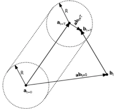
When we have distance based message with a validity interval longer than zero, the situation gets somewhat complicated, since both the sender and the destination objects can move in the space during the validity interval. As mentioned earlier, velocities are constant along a time slot in the dynamic model, so the position of the moving
objects can be calculated with the following formula: t T t ) t ( t T t ) t ( 0 t T t 0 t b 0 t 0 t T t 0 . t a 0 t = = = = = = = = − + = ⋅ + = − + = ⋅ + = b b b v b b a a a v a a (1)
where a and b are the positions of the sender and a possible receiver object, T is the length of the time slot, t is the time elapsed from the beginning of the time slot, R is the message distance and va
and vb are velocity vectors (Fig. 3.).
R at=0 at=T R bt=T bt=0 abt= T abt=0
Fig. 3 Two objects moving in the 3D space and their distance vector
If we take the position of the sender object (2) as reference point, the distance between the objects (ab vector) can plotted against the time elapsed from the beginning of the time slot (Fig. 4): (2) abt=0 ab t=T R abt=t1
Fig. 4 The change of the distance vector (ab) in a timeslot
When the distance between the objects be-comes equal or smaller than the message distance (t≥t1 on Fig. 4) the following expression becomes
true: R ) t ( ≤ ab (3)
This leads to a quadratic equation for t with the following parameters:
(4)
(where velocity and position is now in scalar form)
By solving this equation and examining its roots we can determine the time when two ob-jects get close enough to transmit the message. However, we still not finished yet: it is possible that more than one object gets “close enough” to the sender in the time slot, so we have to check all possible receiver objects with this method. Then, the message must be sent to all receivers object in the calculated order by time.
In case the sender objects is a track object, the situation gets a bit different, since track objects do not move, but are represented by segmented lines, not points. To overcome this problem, a virtual object is created, which moves along the track spline at very high speed. The direction of the movement corresponds to the current route of the track object. With this trick, the problem can be traced back to simple moving point to point messaging explained earlier (Fig. 5).
Route direction R
Track centerline
Fig. 5. Using a track object as sender of distance-based messages
(
) (
)
t t T ab ab ⋅ + = − − − = − = − = = = = = = = = = = v ab ab b b a a v b a ab b a ab 0 t 0 t T t 0 t T t T t T t 0 t 0 t ) ((
)
(
2)
2 0 t z, 2 0 t y, 2 0 t x, 0 t z, abz 0 t y, aby 0 t x, abx 2 abz 2 aby 2 abx R ab ab ab C ab v ab v ab v 2 B v v v A − + + = ⋅ + ⋅ + ⋅ ⋅ = + + = = = = = = =3 SIMULATING TRAIN CONTROL SYS-TEMS
With a flexible simulation architecture, the principles described in the previous section can be efficiently used for simulating all kind of train control systems, including all levels of ETCS. 3.1 Non-continuous train control
Non-continuous train control includes INDUSI variants, ETCS with balises, ZUB etc. These systems can be easily simulated with using simple distance-based messages.
For example, to simulate a line equipped with INDUSI, we need two special objects: - the INDUSI magnet object and
- train on-board equipment (can be integrated in the vehicle object)
The magnet objects are controlled by their corresponding signal object (the signal notifies the magnet whenever the aspect changes). Re-sponding to the periodic message from the kernel, each magnet continuously broadcasts a custom, distance-based message with validity interval of time slot duration, and validity distance of 0.5 meter. The parameter of the message is the current resonating frequency of the track magnet. The required handler program is just a few lines long.
Since magnets can be very relatively close to each other, the message distance must be kept low, and the receiver object must positioned properly.
When vehicle object’s handler program re-ceives the custom message from a magnet, it has to respond by initiating brake curve calculation, emergency brake, speed supervision etc. accord-ing to the magnet frequency.
3.2 Continuous train control with track circu-its
Track circuits are widely used in Europe as transmission medium for train control systems, even on high speed lines (e.g. TVM).
The simulation of such systems like the Hungarian EVM is a complicated task, because the behaviour of track circuits must be accurately simulated.
For this purpose, we use the track objects as “relay” objects. Track objects can be pro-grammed to broadcast a message along the corresponding spline in the direction of the
current route. So, the only thing we have to do is when a track circuit’s feeding signal must change (according to the signal aspect and feeding direc-tion), a notification message is sent to the track object with the new signal identifier as parameter. Then, the track object will broadcast a distance-based “one-shot” message through the “rails”. (“One-shot” means that message is transmitted to only the first possible receiver object in time. This is required for simulating the shunting effect of a train’s first axle.)
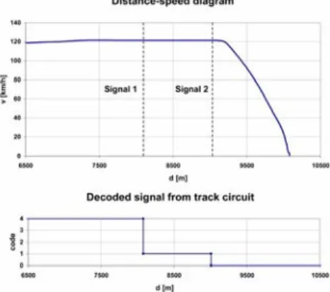
By lowering the simulation step (usually 10 ms), it is possible to do even more accurate tests. The track circuit signal codes can be replaced with High and Low levels, and produce real signal forms. This method also allows adding random noise to the signal, which could be useful for hardware-in-the-loop tests. However, this would require more complex objects.
Fig. 6 shows measurement results of test run with EVM type continuous train control system.
Fig. 6. Test run with EVM type continuous train control system. After passing signal 2, an emer-gency brake intervention occurred.
3.3 Continuous train control with loop Practically, loop-train transmission for sys-tems like LZB, can be simulated in the same way used for track-circuit-to-train transmission. The only difference is that there is no need to simulate the shunting effect, simply all possible receiver objects get the broadcasted message (i.e. no “one-shot”).
3.4 Train control with wireless communicati-on
With the application of ETCS level 2 or GSM-R with other equipments, communication of the train control is done via wireless devices. In most cases, this can be easily simulated with distance based messages with or without addi-tional delay.
In some cases, the wireless connectivity must be seriously considered if the terrain allows its use. This requires very resource-demanding operations: all terrain obstacles must be checked that would cause shielding.
4 CONCLUSION
Throughout the research in the subject of train control simulation, many experiences have been gained which were employed in a powerful software tool. By using the presented methods, all kinds of train control systems can be easily simulated in the system. The application of the developed software in the design and training process can be very efficient, especially when cooperation of different systems must be tested, even with hardware-in-the-loop approach.
In 2003, a Failure Mode and Effect Analy-sis (FMEA) test was carried out with the pre-sented simulation system to examine various level crossings on an ETCS level 1 equipped line (Vincze et al, 2004).
5 LITERATURE
Vincze, B. and G. Tarnai. (2004) Examination of level crossings on ETCS equipped lines with complex simulation. In: AEEE, Heft 5, S.
345-378.
Vincze, B., (2003) Examination of ETCS equipped grade crossings with complex simulation, BUTE Dissertation p1-90 Terada, N. (2003) Application of formal methods
to automatic train control systems. In: FORMS 2003 Conference Proceedings K. Lano, K. Androutsopolous, D. Clark (2003)
Formal specification and verification of of railway systems using UML. In: FORMS 2003 Conference Proceedings
Discreet website: http://www.discreet.com
MXRAIL website: http://www.bentley.com