Experimental Validation of a Phased Array Ultrasonic Testing Probe Model and Sound Field Optimization

(1)

THESIS FOR THE DEGREE OF LICENTIATE OF ENGINEERING IN SOLID AND STRUCTURAL MECHANICS

Experimental Validation of a Phased Array Ultrasonic Testing

Probe Model and Sound Field Optimization

XIANGYU LEI

Department of Industrial and Materials Science (IMS) Division of Engineering Materials

CHALMERS UNIVERSITY OF TECHNOLOGY G¨oteborg, Sweden 2020

(2)

Experimental Validation of a Phased Array Ultrasonic Testing Probe Model and Sound Field Optimization

XIANGYU LEI

ISSN 1652-8565

Chalmers University of Technology SE-412 96 G¨oteborg

Sweden

Telephone: +46 (0)31-772 1000

Cover:

Beam forming in steering and focusing case using a 16-elements linear phased array probe with non-linear delay law

Chalmers Reproservice G¨oteborg, Sweden 2020

(3)

Experimental Validation of a Phased Array Ultrasonic Testing Probe Model and Sound Field Optimization

XIANGYU LEI

Chalmers University of Technology

Abstract

New manufacturing technologies are developed to facilitate flexible product designs and production processes. However, the quality of the final products should not be compromised, especially for safety prioritized industries, e.g. aerospace industry. The assessment of product quality and integrity lies on various nondestructive inspection methods and the ultrasonic testing method, among others, is widely used as an effective approach. The phased array technique in the ultrasonic testing area shows more advantages comparing to conventional ones and is revealing more benefits to industrial applications. To incorporate new technique into practical operations, it needs to be qualified with practical experiments. Due to the extensive costs and considerable challenges with experimental works, the necessity of researching on numerical simulation models arises and several models had therefore been developed. The numerical simulation model implemented in the software, simSUNDT, developed at the Scientific Center of NDT (SCeNDT) at Chalmer University of Technology is one of these models for ultrasonic inspection. However, the validity of the models should be proved before supporting or replacing the experiments, and this validation work should be accomplished by experiments ultimately.

In the current work, the main purpose is to further validate the phased array probe model in simSUNDT by comparing simulation results with corresponding experiments. An experimental platform is built with the intention to fully control the operation conditions and the set of testing results. Well-defined artificial defects in test specimens are considered in both simulations and experiments. Comparisons in the end validate the current phased array probe model and could be treated as an alternative to experiments.

With the aid of this validated probe model, optimization of the generated sound field from a phased array probe is then conducted. The optimization aims at searching for a proper combination of main beam angle and focus distance of the probe at this stage, so that the echo amplitude from a certain defect reaches its potential maximum.

(4)

(5)

Preface

This thesis includes the work conducted during the year 2018 - 2020, which is part of a research projectAdaptive Nondestructive Testing of Additive Manufac-turing (Adaptiv of¨orst¨orande provning vid additiv tillverkning p˚a Svenska). This research project is a collaboration between GKN Aerospace Engine Systems and Chalmers University of Technology, funded by the Swedish innovation agency VIN-NOVA (reference number 2017-04856) within the national aeronautical research program (NFFP7). The actual work was carried out at the research group of Advanced Nondestructive Testing, department of Industrial and Materials Science, Chalmers.

During my studies at Chalmers, I got lots of help from my surroundings. Special thank is given to my supervisor Prof. H˚akan Wirdelius for his great help along the way, and his ideas that always pull me out from my dead ends. He taught me that there is no unique correct answer in researches, but one should try the best to find the way to solve a problem. I also appreciate the help from Anders Rosell from GKN in all forms of discussion about my work. The technical helps from Farham Farhangi and Daniel Sn¨ogren from the Swedish Qualification Centre (SQC) are also highly appreciated when I first touched the experimental work and software. Furthermore, I also want to say thanks to other members in our research group, it is good to share the Fika time with them!

Finally, I am really grateful to my beloved family that always support and encourage me in China, and to my best friend Hao Wang staying with me when I was in hard time.

Gothenburg, 2020 Xiangyu Lei

(6)

(7)

Thesis

This thesis consists of an extended summary and the following appended papers: Paper A

Xiangyu Lei, H˚akan Wirdelius, Anders Rosell. ”Experimental Validation of a Phased Array Probe Model in Ultrasonic Inspection”.

Submitted for publication

Paper B

Xiangyu Lei, H˚akan Wirdelius, Anders Rosell. ”Experimental Validation and Application Of A Phased Array Ultrasonic Testing Model On Sound Field Optimization”. Submitted for publication

The appended papers were collaboratively prepared with co-authors. The author of this thesis was responsible for the major progress of the work, i.e. designing and performing of experiments, simulations, post-processing and writing of the papers, all with the assistance of the co-authors.

(8)

(9)

Part I

Extended Summary

1

Introduction

Ultrasound as a method of nondestructive evaluation (NDE) and nondestructive testing (NDT) has been used for centuries in both medical and industrial fields thanks to its rapid and safe characters.

Ultrasound or the ultrasonic wave, as indicated by its nomination, is the sound wave that vibrates at frequencies over 20 kHz. Typical frequencies used in ultrasonic NDE applications are ranged from 50 kHz to some MHz. The fundamental theory of using ultrasound to perform evaluation and characterization is that the sound waves can propagate in solids, liquids and gas. The features, such as propagation velocity and attenuation of the sound waves, can be used to characterize the material properties in terms of its structure, elastic properties, etc. When propagating in an object, the waves interact differently to the variations in the object, for example in a fabricated structure, when encountering a pore (air) that has a different density compared to the surrounding structures, the waves scatter as echoes, so that one can detect these echoes and have an understanding of the different composition inside the object.

Today, many industries are using ultrasound as one of the inspection media that ensure the structural integrity and quality of the manufactured components. New techniques in this area are continuously developing along with the arising and application of the new manufacturing technologies.

1.1

Background

In aerospace industries, in order to fulfill the increasing demands of aeroengines manufacturing with low environmental impact and reduced fuel consumption, advanced production and lightweight technologies are developed, e.g. additive man-ufacturing (AM). This new technology enables effective manman-ufacturing, materials utilization and energy optimization, which is suitable for lightweight components production. However, new manufacturing methods come along with problems, e.g. heat caused deformation and the appearance of unknown vital defects inside the components specifically related to the production process. Thus, the application of these new production technologies demand higher and more reliable inspection methods for quality insurance and to maintain certain safety margins. In com-mon sense, destructive testing (cut-up) is one way of accomplishing it, but it is

(12)

expensive, time-consuming and obviously, the destroyed components should not be used any longer and is not suitable for small quantity of objects. To overcome these drawbacks and to ensure the quality at an early stage as well as reducing production costs, NDT methods should be considered.

Ultrasound, or refer to Ultrasonic Testing (UT), among others, has been proven to be an effective and powerful inspection method within this context. The phased array technique in this area, referred to Phased Array Ultrasonic Testing (PAUT), is even more advanced that enables more flexible and faster operations, which compared to the conventional single-element UT has the possibility of enhanced signal-processing.

Before applying the new inspection techniques and evaluation procedures, comprehensive qualifications must be performed for both NDT techniques and related personnel [1]. Traditionally, the qualification processes are based on extensive experiments towards actual test specimens, which means that many variables should be characterized and limited to situations related to the specific application scenario. In addition to the massive cost of producing representative test specimens, the challenges of manufacturing characterized defects in critical locations are considerable. Such experiments could however, be assisted or even partly be replaced by mathematical models that had been developed in recent decades [2, 3]. These models include such as CIVA [4, 5], Thompson-Gray Measurement Model used in UTSim [6], Finite Element Method (FEM) model [7, 8], Elastodynamic Finite Integration Technique (EFIT) [9, 10], etc. With the help of these models, the corresponding experiments can be emulated numerically and the involved physical principles can be studied for further development. For instance, Azar et al. [11] took advantage of a numerical model to simulate the pressure field of a PA probe in beam steering and focusing cases, to show e.g. the impact of focusing to detection resolution in the near field. Puel et al. [12] utilized numerical simulation with a evolutionary algorithm based optimization method to reach an optimal design and setting of phased array probe. Other similar studies can be seen in e.g. [13, 14].

However, the numerical models should be thoroughly validated before practical use. This is performed either by comparing the model with other models that had been validated, or by comparing the model with experimental results, which should ultimately be done in order to show that the model truly reflects the reality [15, 16].

The UT simulation model developed by Chalmers University of Technology is implemented into software, simSUNDT [17]. The conventional probe model involved has been validated [18–20] by comparing the simulation with the experi-mental benchmark study [21], which was started by the World Federation of NDE Centres and the experimental results were provided by Commissariat a l’´energie

(13)

atomique (CEA, France). The PA probe model [22] however, was validated only to a limit extent and thus requires further validation work. After the PA probe validation, the model is capable of facilitating the sound field optimization in order to get the maximized echo amplitude towards a defect, performed in the present work.

1.2

Aims and limitations

This thesis is part of a research projectAdaptive Nondestructive Testing of Additive Manufacturing, which has the overall objective to incorporate the developed tools into inspection technologies during manufacturing processes, with the intention of quality control and assessment. The tool should also be optimized towards well-defined manufacturing defects, which potentially may occur in manufacturing processes. To accomplish this goal, the ultrasonic wave propagation within complex geometries should be studied through corresponding mathematical models. The overall research questions are hereby lie on e.g., how well the mathematical models can reflect on the physical inspections, what flexibility can be provided by the models, how can the models help with production and process optimizations, etc. The present work is thus focused on further experimental validation of the newly developed PA probe model in the software, simSUNDT. The experiments are performed at the NDT lab of the Scientific Center of NDT (SCeNDT) at Chalmer University of Technology using a newly built mechanized operation platform. After the validation of the model, it is then used to investigate the approach of sound field optimizations towards a backwall surface breaking defect, with the intention to retrieve a maximized corner echo. This is mainly conducted by adjusting the combination of beam angle and focus distance of a PA probe, to optimize the sound field for specific defect characteristics at this stage.

However, some limitations are involved. In the validation work, the considered defects only address well-defined artificial ones, i.e. SDH and surface breaking defect. Source of attenuation including material damping properties of the test specimen and contact conditions that could influence beam divergence characters are not included in the corresponding simulations, because the validation focus is on the PA probe model instead of material properties. These limitations could provide error source to the validation results.

1.3

Thesis structure

This thesis is structured in following sections according to the aims. Section 1 provides background information as well as the objectives and limitations of the

(14)

current work. Section 2 introduces basic knowledge related to the ultrasonic testing method. The software simSUNDT is also briefly introduced with theoretical base and capabilities. Section 3 presents a simple and general approach to phased array delay law derivation based on geometrical wave path compensation. Section 4 summarizes the practical information of experiments used in probe model validation work. Section 5 gives an overview of the optimization work and the applied algorithm. Section 6 lists the summary of appended papers. The extended summary ends with Section 7, where some concluding remarks are provided with the future direction of work.

2

Technical Background

2.1

Ultrasonic Testing (UT)

2.1.1 Basic principles of ultrasound generation and receiving The ultrasonic testing method is all based on the ultrasonic waves, which is gener-ated from a specific transducer or probe. The essential part inside a conventional probe is the piezoelectric element that converts the imposed electrical pulse into mechanical movement of the element, and vice versa. The vibration frequency of this element is determined by its thickness as indicated by equation (3.98) in [23], i.e. the thinner the element, the higher the frequency. When the element is vibrating, a pulse of sound will be generated in the adjacent medium (solid, liquid and gas) in the form of acoustic waves. The waves can propagate within the medium and scattered if strikes an object, e.g. pore or inclusion, which has a differentacoustic impedance comparing to the surrounding medium. The scattered waves then travel in all directions depending on the property of the object and some of them return back to the probe. The piezoelectric element receives the vibration and converts it back to electrical pulse, which is then amplified as the output signal. This signal is represented as pulse amplitude versus elapsed time. By knowing the wave traveling speed in the medium, the line distance between the probe and the object can thus be determined. Therefore, the ultrasonic testing method, like all other NDT methods, is indirect by nature, i.e. the measured out-puts are in the form of pulse vs. time and that other quantitative information are not directly obvious, e.g. the size of the object, which need further interpretations. Nevertheless, the quantitative information could be determined to some extent in post-processing if moving the probe to collect signals from different positions and orientations.

(15)

2.1.2 Near field and far field

As the piezoelectric element converts an electrical pulse into mechanical movement, the generated sound waves travel along their paths. Due to the reason that the actual element is not a point but has an area, the waves generated from each point of the area must have different path lengths along the traveling direction, which cause interference both constructively and destructively that end up with intensity fluctuations in a short distance. The region within this distance is called

near field and beyond that is calledfar field, where the wave path differences are smaller, leading to minor intensity fluctuations and the intensity decreases slowly with growing distance, as expected. The near field length N for a certain probe can be expressed by:

N = D

2

4λ (2.1)

whereλis the wavelength and D is the diameter of a circular probe.

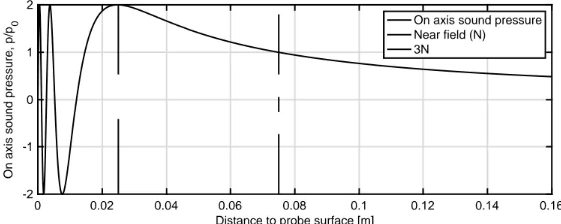
As a simple example, the normalized sound pressure level along the axis of a piston oscillator, on which the displacement is the same for all points, can be seen in Figure 2.1 [24], wherep0 is the average pressure value in the near field region.

It is seen that the sound pressure level fluctuates in the near field and reaches its last maximum at near field length. After that, the pressure decreases slowly as the distance increases and returns to the average pressure level at the third times of the near field length. Practically, most experiments are performed in the far field due to the nature of unstable wave pressure in near field.

0 0.02 0.04 0.06 0.08 0.1 0.12 0.14 0.16

Distance to probe surface [m] -2

-1 0 1 2

On axis sound pressure, p/p

0 On axis sound pressure

Near field (N) 3N

Figure 2.1: Sound pressure variation along the axis of a piston oscillator as a function of distance to the probe surface

(16)

2.1.3 Wave types

For sound waves, there are two types of traveling in bulk materials, namely

longitudinal waves and transverse waves. They are differed by the movement directions of the medium particles. There are however other types of waves, such as Rayleigh waves and Lamb waves, also available for certain inspection purposes [23], but the longitudinal and transverse waves are mostly used in ultrasonic testing.

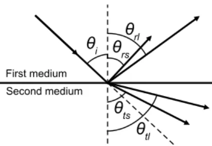
Different wave modes can be converted. This phenomenon is called mode conversion, which happens when the waves strike on the material interface at an oblique angle. The waves are reflected in the same medium, calledreflection, but it can also travel into the second medium, calledtransmission. It should however be noted that the mode converted waves will propagate in a different direction, which can be determined through Snell’s law. This law is used to determine the direction (angle) of reflected and transmitted mode-converted waves when the waves strike on the material interface at an oblique angle. Refer to Figure 2.2 it can be expressed as:

sinθi vi = sinθrs vrs = sinθrl vrl = sinθts vts = sinθtl vtl (2.2) where

θi - incident wave angle

θrs - reflected transverse wave angle

θrl - reflected longitudinal wave angle

θts - transmitted transverse wave angle

θtl - transmitted longitudinal wave angle

v is the wave speed in corresponding medium for each case

Figure 2.2: Wave mode conversion and Snell’s law demonstration

It is worth mentioning that the Snell’s law only shows the propagation directions of the waves without any information on their amplitudes. Looking at Snell’s law, it can be noticed that when the transmitted wave angle reaches 90°in the second

(17)

medium, it would propagate along the material interface. This corresponding incident wave angle is thus called the critical angle. Knowing the fact that the longitudinal waves generally travels faster than the transverse waves in mediums, the longitudinal wave angle should be larger than the transverse wave angle. 2.1.4 Data presentation

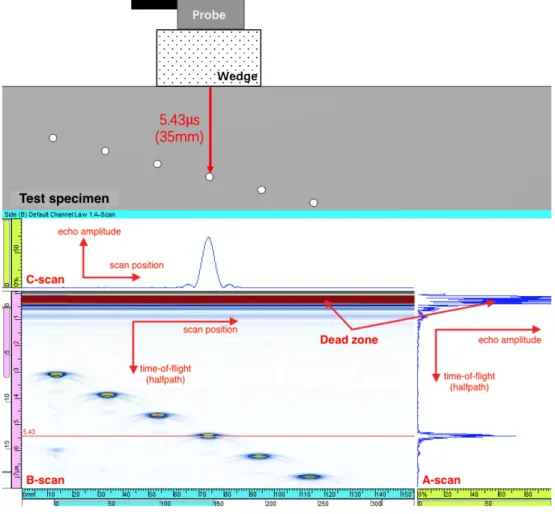
As mentioned in Section 2.1.1, the ultrasonic testing is an indirect method since the result presentations need to be post-processed before interpretation. The direct variables used in conventional inspections aretime-of-flight and amplitude. All other information and result presentation formats are derived based on these variables. Conventionally, there are three formats used to visualize the inspec-tion results, known as A-scan, B-scan and C-scan, each of which presents the data in a different way for evaluation, see an inspection example in Figure 2.3. Previously mentioned pulse amplitude vs. time-of-flight direct presentation is denoted as A-scan, directly obtained through inspection equipment and provides a straightforward echo indication at which distance an object exists. B-scan shows a cross-section view of the test specimen. It is generated by re-organizing and color-scaling an A-scan amplitude along the vertical axis (time-of-flight axis) at a scan position, and repeating for all scan positions of the probe along the horizontal axis. In this way, given the wave speed in the test specimen, the depth of the defect and its approximate linear dimension in the scan direction can be deter-mined. C-scan shows a color-scaled top view of the defects in test specimen for a raster scanning sequence, parallel to the scanning surface. It is obtained through color-scaling the maximum echo amplitudes at each scanning position. C-scan can also be an echo dynamic curve for an one-line scanning sequence, showing the maximum echo amplitudes at each scan position (the case in Figure 2.3). It is useful when presenting the defect distribution in the scan plane. Obviously, the scanning position information is needed to generate the B-scan and C-scan. With a modern ultrasonic inspection equipment, together with a mechanized system equipped with encoders providing probe position information, it is possible to visualize these scan presentations simultaneously during real-time inspection. 2.1.5 Probe configuration

Basically, there are two ways to configure the ultrasonic probes during inspections depending on the number of probe/probes used. If only one probe is used for both generating and receiving the waves, it is calledpulse-echo mode. This mode simplifies the overall experimental setup, but thedead zone occurs in the received signals, shown in Figure 2.3. The dead zone refers to a region where the initial

(18)

Figure 2.3: An example of inspection situation, where the current probe center sits above a defect (35 mm depth). The results are presented in A- B- and C-scan (echo dynamic curve in this case of a one-line scan) and the dead zone is also visible in A- and B-scan

large electrical pulse generating the waves is also treated as a received signal, which has a large initial echo amplitude in the result presentations. It can totally mask an echo from a real defect within this depth region of the specimen. This drawback can be overcome if one probe is used for generating the waves while another probe is for receiving at a different position along the wave path, called

pitch-catch mode, because the initial large electrical pulse will not be detected by the receiving probe. This mode is therefore more appropriated for near-surface defects detection and detection on thin materials. Time of Flight Diffraction Technique (TOFD) is one of the examples using pitch-catch configuration.

(19)

2.2

Phased Array UT (PAUT)

The phased array (PA) configuration generally refers to a series of transducers in an array setup, ordered linearly or in matrix form. Phased array ultrasonic testing

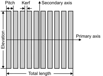
(PAUT) therefore refers to an ultrasonic testing method that utilizes the specific probes, which consist of an array of small piezoelectric elements. The element shape is in most cases rectangular since they are cost-effective to produce, which is used in two types of arrays, namely linear and 2D arrays based on how the individual rectangular elements are arranged. Figure 2.4 for example, shows a sketch of a linear PA probe surface with corresponding terminologies used in this field. There are also other types of PA probes with overall angular shapes [25] in PAUT, but the linear and 2D arrays are most generally used in NDE.

Figure 2.4: The terminology of a linear phased array probe

Each of these small elements can be triggered individually by electronic pulse, and the signal response can also be received independently. The advantages of this configuration comparing to the conventional single-element UT are revealed by the flexibility of sound beam steering and focusing through constructive interference of waves, together with the possibility of fast visualization generation [25]. As it is known for conventional single-element UT, the beam steering and focusing is accomplished by using corresponding wedge that has an angle or curved, which needs to be applied based on a certain application scenario. Whereas for the PA probe, each element can be driven separately, thus it is of nature that there can be linear time shifts between pulses. The individual small element now approximates as a point source that emits spherical waves, while the generated synthetic wave front after constructive interference is hereby a plane wave and can travel in

(20)

different directions based on different combinations of time shifts. This time shifts combination is called delay law, and its general derivation is seen in Section 3. Furthermore, if the applied delay law is nonlinear, the generated wave front can also emulate the focusing effect, just as the conventional single-element ultrasonic probe with a curved wedge, that the sound beam is focused at a certain point where the sound pressure reaches maximum. The beam steering and focusing can also be combined in more complex operations if needed.

When each of these elements receive signals, the corresponding time delay laws generally can also be used to shift the individual signals so that all of them appear at the same time and can be summed up to obtain a single and large signal in the end. Thus, in this transmitting and receiving process with proper delay laws, the effect of using a PA probe is the same as using a conventional single-element probe associated with the corresponding angled or curved wedge. The advantage of using a PA probe is that the beam steering and focusing effect are obtained simply by adjusting the proper time delay laws, with no need of moving or changing the physical probe as in the conventional inspections. This flexibility enables many ultrasonic measurements in a rapid and simple way, for example a rapid sectorial scan in a region using a single PA probe and real-time imaging based on acquired data. Figure 2.5 shows an inspection case as an example, using a single PA probe on an AM component (Titanium Alloy 6AL4V) with side-drilled holes (SDHs) at depth of 14 mm. The SDHs under inspection have diameters of 1.2 mm, 0.8 mm and 0.4 mm from left to right. The probe contacts directly on the surface and its position is unchanged as shown in the figure. The delay laws together with the pulse sequences applied are: (a) 16-elements aperture travels linearly along the array without focusing effect; (b) 16-elements aperture travels linearly along the array with focusing at SDHs; (c) 64-elements aperture sectorial sweeping from -45° to 45° with focusing at SDHs and (d) Full Matrix Capture (FMC) that will be introduced in Section 2.3. The corresponding data visualization in B-scan can be seen in Figure 2.6, where the FMC data is visualized using an advanced imaging algorithm, Total Focusing Method (TFM), also introduced in Section 2.3. It can be noticed in Figure 2.6(a)-2.6(c) that weaker ghost indications are also visible below the SDH indications, which probably come from bottom sphere reflections, whereas the ghost indications are eliminated in Figure 2.6(d) by TFM.

The near field length of a general rectangular PA probe can also be calculated using equation (2.1), where the probe diameterDis now the total length of the PA probe (see Figure 2.4) if the aspect ratios between the total length and the elevation is larger than 0.6 [13]. By focusing effect, the resolution within PA probe’s near field can be improved [11], as compared by Figure 2.6(a) and Figure 2.6(b). It is also noted that the generated sound beam in the far field is similar to the one generated by the conventional single-element probe that has the same

(21)

Figure 2.5: PA probe inspects an AM component with SDHs (diameter of 1.2 mm, 0.8 mm and 0.4 mm from left to right) at depth of 14 mm from scanning surface

(a) Linear scan without focus (b) Linear scan with focus at SDHs

(c) Sectorial scan (d) TFM algorithm

Figure 2.6: Four B-scans of flexible scanning and imaging possibilities using PA probe on an AM component with SDHs in the middle, as the case shown in Figure 2.5

(22)

overall size as the PA probe. Because of these advantages, PAUT had been applied in medical applications since decades [26, 27] and is now attracting more attentions from the industrial perspectives. For example, Shan et al. [28] built up an PAUT inspection system for defect detection in steel structures. A SDH in the test block can be quantitatively evaluated from the system. Lopez et al. [29] explored the possibility of using PAUT on AM component inspections and it was concluded to be suitable also for quantitative evaluations. Qin et al. [30] introduced an improved delay law calculation for PAUT technique based on the relation between the observed peak offset and propagation distance in high-density polyethylene used in the nuclear power plant pipes, in order to improve the ultrasound field intensity at the focal point of interest and to increase the imaging sensitivity. Gros et al. [31] discussed about more applications and the advantages of using PAUT in industries, as well as the necessity of numerical modeling and some future development possibilities of the technique.

2.3

Full Matrix Capture (FMC)

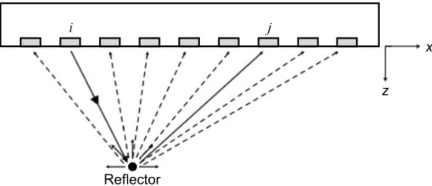
Using an ultrasonic PA probe,Full Matrix Capture (FMC) is a data acquisition method capturing complete set of time-domain signals from each possible pair of transmitter-receiver combination, e.g. time-domain signal fromi-th element (transmitter) toj-th element (receiver),Sij, illustrated in Figure 2.7. For an array

with N elements, FMC can generateN2 _{possible time-domain data. With this}

complete set of data, any beam-forming scheme of conventional PAUT can be emulated in the post-processing with no need of further experiments.

Figure 2.7: Full Matrix Capture (FMC) illustration

To fully use the FMC data, an imaging algorithm called Total Focusing Method (TFM) is preferred, which has better imaging performance comparing to conventional algorithms [32], see also comparisons in Figure 2.6. TFM is

(23)

performed by firstly discretizing the imaging region of interest into frame grids, then advancing all pairs of FMC signals using the corresponding time-of-flight of this pair to the imaging grid point. The image is finally formed by summing these signals at time t= 0 and repeating for all image grid points. Due to the massive computation effort, TFM imaging is practically performed during post-processing.

2.4

simSUNDT

The simSUNDT software consists of a Windowsr-based pre- and post-processor, as well as a mathematical kernel UTDefect [19, 33] that conducts the actual mathematical modeling and computation. UTDefect was developed at Chalmers University of Technology. The 3D elastodynamic wave equation, which defines the wave propagation in a homogeneous half space, is solved using vector wave functions [33].

The contact probe can be modeled in elliptic and rectangular shape. The modeling assumes that the probe is placed on the surface of an elastic half-space, which has no traction on the surface except beneath the probe. This enables the possibilities of simulating any types of the probe available on the market, by specifying related parameters such as wave types, element size and shape, angles, frequency ranges, contact conditions, etc. The traction is derived so that a plane wave is generated in the far field, shown in equation (2.3) for longitudinal, vertical transverse (SV) and horizontal transverse (SH) wave types, respectively.

t=                Agiµkp[( k2 s k2 p −

2 sin2γ)ˆz+δsin 2γxˆ]e−ikpxsinγ_,_{Longitudinal probe}

Agiµks[sin 2γzˆ−δcos 2γxˆ]e−iksxsinγ,SV probe

Agiµksδcosγyeˆ −iksxsinγ,SH probe

0,elsewhere

(2.3)

where ˆx, ˆy and ˆz are the unit vectors in corresponding directions. A is the displacement amplitude and the function genables reduction of edge effects. µ

is the Lam´e constant of the elastic half space. kp and ks are longitudinal and

transverse wave numbers, respectively. γ is the wave angle. δ _∈ [0,1] is a constant that represents the coupling effect, where δ=0 is fluid coupling andδ=1 is glued condition.

The wave propagation is governed by the elastodynamic equation of motion, in which the displacement field, u, is involved:

k−2

(24)

The total displacement field is a summation of the incident field (ui) and the scattered field (us), as:

u=ui+us (2.5)

The incident fields can be expanded in terms of regular spherical partial vector waves (ReΨn), and the scattered field caused by various of defects can be expanded

in its outgoing spherical partial vector waves (Ψn):

       ui=X n anReΨn us=X n fnΨn (2.6)

Volumetric and crack-like defects are available types of defect to be modeled. Specifically, volumetric defects include a spherical/spheroid cavity (pore), a spher-ical inclusion (isotropic material differing from the surrounding material, i.e. slag) and a cylindrical cavity (SDH). Crack-like defects include rectangular/circular crack (lack of fusion) and strip-like crack (fatigue crack). There is option to model the surface roughness for the rectangular and strip-like crack, and the degree of closure can be modeled for the circular crack. Tilting planar back surface could also be modeled for the strip-like crack, but otherwise it is assumed parallel to the scanning surface. The surface-breaking strip-like crack and rectangular crack close to the back surface can be used to model the corresponding defects in the test piece.

The modeling of these defects are important and the methods of solution can be for example, various types of surface integral equations, null field approach (T-matrix method) and FEM. UTDefect incorporates the T-matrix method [34] and all information regarding the defects is included in the transition matrix, as well as providing the linear relation between the expansion coefficients of the incoming (an) and scattered (fn) wave fields in equation (2.6):

fn=

X

n0

Tnn0a_n0 (2.7)

To incorporate the probe model into the T-matrix formulation, the displacement field needs to be transformed from the plane vector waves centered at the contact area into spherical vector wave functions oriented and centered at the defect [33].

To model the receiver, a reciprocity argument [35] is applied. In the end, the electrical signal response is expressed by:

δΓ∼X

nn0

(25)

With the transmitting probe is characterized byaa

n0, the defect byT_nn0 and the receiving probe byab

n.

To simulate the entire testing procedure of an actual NDT situation, a cal-ibration option is available towards a reference reflector including for example, the side-drilled hole (SDH) represented by the cylindrical cavity [36] and the

flat-bottomed hole (FBH) approximated by an open circular crack.

The model geometry can be limited by a reflecting backwall and be described as a plate with finite or infinite thickness bounded by the scanning surface, on which the scanning sequence are defined by rectangular mesh.

In addition, it is also possible to suppress the unexpected wave component in the simulation to eventually facilitate the analysis of the received signal. The configurations of the probe can be chosen among pulse-echo, separate with fixed transmitter and tandem configuration (TOFD).

These principles are the same for the phased array probe model, that element is represented by the boundary conditions (traction), from which the plane wave is generated in the far field with a certain angle. The individual boundary conditions are translated into the main coordinate system and a phased array wave front with certain nominal angle is formulated by constructive phase interference. The formulated nominal angle can also be altered by specific delay law, but it should be noted that this is only possible for small angles if no wedge is specified.

3

Delay law derivation

As mentioned in Section 2.2 that the delay laws are used to steer and focus the generated beams for the PA probes. It is easy to imagine that a focusing effect by nature requires also beam steering of some probe elements. In other words, beam steering can be treated as a special case to beam focusing with infinite focusing length. In this section, the general delay laws for linear PA probe are derived for both beam steering and focusing. It is basically done by compensating for the geometrical wave path lengths between each element, as each element of the array emits a wave that travels in a straight line at high wave frequencies [37].

Before the derivation, some nomenclatures of the normal parameters used for the PA probe, the wedge, material properties and inspection case are firstly introduced in Section 3.1. The wedge is generally involved in practical applications that facilitates the mechanized operation and coupling possibilities, and the first element of a PA probe is set to the lower edge side of the wedge, to be consistent with the actual industrial application. For more general cases, an angled wedge is used in these derivations.

(26)

3.1

Nomenclatures

Below lists the nomenclatures specifically used for these derivations. It should be noted that all these parameters are known before specifying a delay law, except for Φ1 inside the wedge.

Table 3.1: Nomenclatures used specifically for delay law derivations

Notation Nomenclatures

N Total number of elements in a PA probe

p Pitch between elements

Wedge angle

h1 Vertical distance of the center of the first element to the wedge bottom

c1 Wave speed in the first medium (wedge)

c2 Wave speed in the second medium (test specimen)

Df Vertical focusing depth from the surface of test specimen Φ1 Primary beam impinging angle in the first medium (wedge)

Φ2 Refracted (expected) beam angle in the second medium (test specimen)

3.2

Beam steering

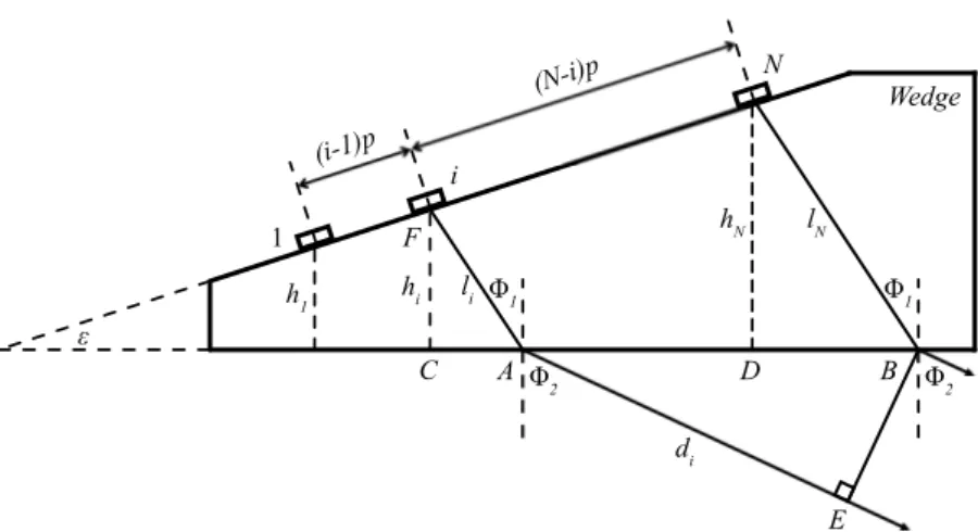
The geometrical parameters used in beam steering case are indicated in Figure 3.1. Assume that all probe elements on the wedge surface are activated in the beam forming process. For this pure steering case, the generated wave should be a plane wave, which means that each wave path should be in parallel with each other and propagates in a specified refracted angle Φ2 in the second medium.

Take the i-th and the last element for example, the generated wave front in the second medium should thus be represented by line BE in Figure 3.1, which is perpendicular to all wave paths. To accomplish that, when the wave from the

i-th element reaches pointE, the wave from the last element should just reach point B. The time difference between these two waves should therefore be the time delay of the wave that has the shortest time of flight, so that all waves reach the wave front at the same time. Based on this principle, the time of flight of the

i-th wave can be derived and the delay law is obtained.

As indicated in Figure 3.1 that the distance on the wedge surface between the

i-th element and the first element is (i₋1)p, and to the last element is (N ₋i)p, thus the height of the center of the i-th element (point F) to the wedge bottom (pointC),hi, can be expressed by:

(27)

Figure 3.1: Geometrical parameters for delay law derivation in pure steering case

The wave path length for the i-th element in the wedge,li, from the center of

this element (pointF) to pointA (intersecting point between the wave path and the wedge bottom) is expressed in term of hi by:

li = hi cos Φ1 = h1 cos Φ1 +p(i₋1) sin cos Φ1 (3.2) Using equation (3.1) for thei-th element and the last element, the horizontal distance between the center of the element and its intersecting point, CAi and

BD, respectively, can be expressed by:

CAi =hitan Φ1 = [h1+ (i−1)psin] tan Φ1 (3.3)

BD=hNtan Φ1= [h1+ (N −1)psin] tan Φ1 (3.4)

The horizontal distance between thei-th element and the last element, DCi,

can be written as:

DCi = (N −i)pcos (3.5)

Combining equations (3.3), (3.4) and (3.5), the horizontal distance between the intersection pointsA andB for the i-th element and the last element,BAi,

can finally be written as:

(28)

Then, using equation (3.6) the wave path length of the i-th wave in the second medium,di, can be expressed by:

di =BAisin Φ2=p(N −i)(sintan Φ1+ cos) sin Φ2 (3.7)

Combining equation (3.2) and (3.7), the time of flight of thei-th wave from the element center (point F) to its corresponding point E, indicated in Figure 3.1, is expressed by: ti = li c1 + di c2 = 1 c1 h1 cos Φ1 +p(i₋1) sin cos Φ1 + 1 c2

[p(N₋i)(sintan Φ1+ cos) sin Φ2]

(3.8)

Finally, the time delays ∆ti are obtained simply through subtracting all the

individual time of flight,ti (i=1, ..., N), by the largest one:

∆ti =ti−max(ti) (3.9)

For example in a simple case, a PA probe with 5 elements: time of flight, ti: 5µs, 4µs, 3µs, 2µs, 1µs;

time delay,_|∆ti|: 0µs, 1µs, 2µs, 3µs, 4µs

It is worth noting from the equation (3.8) and (3.9) that, the time delays between elements are a linear relation for pure steering case.

3.3

Beam focusing

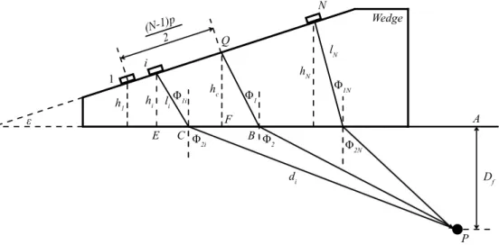
When the beam focusing effect is considered in the delay law generation, the goal is to have all refracted waves reach a common point at certain depth,Df, in the

second medium, which is thefocusing depth one expected and specified in advance. Unlike the pure steering case, since the refracted waves are not in parallel in the focusing case, the corresponding primary impinging waves inside the wedge should not be in parallel either. In other words, each wave path has a different unique impinging angle at the wedge bottom. This is very important to notice because all the impinging angles are not the same as the one calculated by Snell’s law using the nominal refracted angle Φ2. This specified nominal refracted angle Φ2

in practice however, refers to the refracted angle of the overall synthetic wave beam axis in the second medium, see Figure 3.2.

The corresponding nominal impinging angle, Φ1, calculated by Snell’s law in

(29)

Figure 3.2: Illustration of the nominal refracted angle in beam focusing case

in the wedge, represented by a line from the center of active aperture on the wedge surface (pointA) to the synthetic beam exit point (pointB) at wedge bottom. This exit pointB is hereby determined provided that the center of active aperture and Φ1 are known. Note that the lineAB does not have to be a wave path of any

element but it is a representative of the overall synthetic sound beam in beam focusing case.

Understanding the above principles, the time-of-flight of each wave and the delay law derivation for focusing case are followed, refer to Figure 3.3, where the geometrical parameters are indicated. Assume again that all probe elements are active on the wedge surface in this focusing case.

Figure 3.3: Geometrical parameters for delay law derivation in focusing case

Since the vertical focusing depth Df and the expected refracted angle Φ2 are

(30)

and the synthetic main beam exit point (pointB), AB, is a known value:

AB=Dftan Φ2 (3.10)

For the main beam path, the horizontal distance between the center of active aperture on the wedge surface (pointQ) and the main beam exit point (point B),

BF, can be calculated based on the height of pointQto the wedge bottom. This vertical distance, hc, is expressed in a similar way as equation (3.1):

hc=h1+ (N₋1)p 2 sin (3.11) BF =hctan Φ1 = h1+ (N −1)p 2 sin tan Φ1 (3.12)

Then, the horizontal distance between the center of the i-th element and the center point of the active aperture (pointQ), F Ei, is expressed by:

F Ei = (N −1)p 2 −(i−1)p cos (3.13)

It can be seen from equation (3.13) that the value of F Ei for the elements

locate after the aperture center point are negative. Combining equation (3.10), (3.12) and (3.13), the horizontal distance between the focusing pointP and the

center of thei-th element can generally be written by:

AEi =AB+BF+F Ei (3.14)

As mentioned earlier and refer to Figure 3.3 that each wave impinging the wedge bottom at an unique angle, i.e. Φ1i 6= Φ1, and refracted at a corresponding unique

angle, i.e. Φ2i6= Φ2, for thei-th wave, it is thus no ease to determine the impinging

point for an individual wave. However, there should be an impinging point for the

i-th element (pointC) that satisfies the Snell’s law for its corresponding angles Φ1i and Φ2i, namely [37]: sin Φ1i c1 = sin Φ2i c2 (3.15) Using equation (3.1) for element height, hi, to rewrite the equation (3.15) and

(31)

write it as a function of the unknown variable ECi for thei-th element,f(ECi): f(ECi) = sin Φ1i c1 − sin Φ2i c2 = ECi li 1 c1 − ACi di 1 c2 = _q ECi EC2 i +h2i 1 c1 − AEi−ECi q (AEi−ECi)2+D_f2 1 c2 (3.16)

Finding a value ofECi that makes the equation (3.16) equals to zero means

that the Snell’s law in equation (3.15) is fulfilled, thus the impinging point Ci for

thei-th element is found. Furthermore, its corresponding angles are found by: Φ1i = arctan( ECi hi ) Φ2i = arctan( AEi−ECi Df ) (3.17)

Using equation (3.17), the wave path length of thei-th element in both mediums can be expressed by:

li = hi cos Φ1i di = Df cos Φ2i (3.18)

Thus, the time-of-flight of the i-th wave from its element to the focusing point can be calculated using the equation (3.18):

ti = li c1 + di c2 (3.19) Finally, the same as in the pure steering case, the corresponding delay law for focusing case can be obtained using equation (3.9).

4

Experimental setup

This section summarizes the experimental setup, including the UT equipment, the mechanized gantry system, the test specimens used in the experiments, and the design of experiments.

(32)

4.1

UT equipment

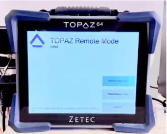
The UT equipment mainly includes the data acquisition hardware (TOPAZ64) and a commercial PA probe with corresponding plastic wedges.

TOPAZ64 (Figure 4.1) is a portable 64-channel phased array ultrasonic testing equipment with FMC and TFM capabilities incorporated. Ultrasonic inspection data is communicated in real time between TOPAZ64 and computer by Gigabyte Ethernet cable connection, and is processed by corresponding software UltraVision on the computer.

Figure 4.1: Data acquisition hardware unit, TOPAZ64

The commercial ultrasonic probe from Zetec is a 64-elements linear phased array longitudinal-wave probe with the notation of LM-5MHz. The nominal center frequency is 5 MHz and bandwidth is 74%. Refer to Figure 2.4, each element has a size of 0.5 mm along primary axis and 10 mm in secondary axis (elevation). The kerf between elements are 0.1 mm and the total aperture of the probe is thus 38.3 mm in primary axis and 10 mm in elevation.

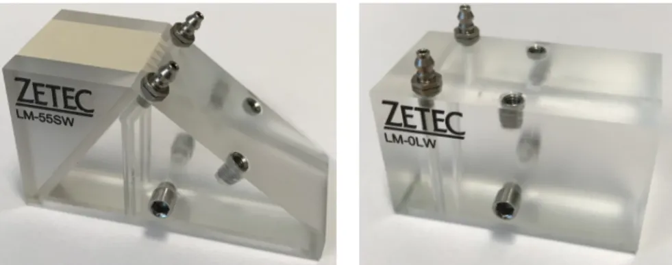
Two specific plastic wedges (Figure 4.2), with and without wedge angle denoted as LM-55SW and LM-0LW, respectively, are used in all experiments to protect the surface of the PA probe and to generate angled beam properly. The skew holes on two sides of the wedge facilitate fixation of the probe on mechanized system, and the skew holes on the wedge surfaces are used to fix the PA probe. The angled wedge (LM-55SW) helps the probe generate 55°transverse waves into carbon steel (wave speed = 3230 m/s) without any delay law, or 40° to 70°transverse waves

(33)

Figure 4.2: Plastic wedges, LM-55SW (left) and LM-0LW (right)

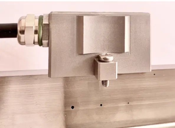
Figure 4.3: Mechanized gantry system on the experimental platform (left) and probe fixation (right)

4.2

Mechanized gantry system

The mechanized gantry system is built on the experimental platform (Figure 4.3 (left)) in order to provide a stable inspection condition with high repeatability between experiments. Currently, the system is motor controlled only in the horizontal plane (x-y plane), while the z-axis position is manually adjusted by a guide skew on top. The embedded encoders in the motors can provide z-axis position information within x-y plane, which enable different data presentation probabilities, e.g. B- and C-scan. The water tank containing test specimens is placed on the platform and the wedge with probe is clamped on the z-axis by a spring-loaded fork, as shown in Figure 4.3 (right).

(34)

4.3

Test specimens

Three flat surface test specimens (#1, #2, #3) with well-defined artificial defects are used in the validation work. One (#1, aluminum) with 15 SDHs (3 mm in diameter) at depth range from 20 mm to 90 mm in step of 5 mm, drilled through the width of specimen and one of the SDHs can be used as calibration defect. As mentioned in Section 2.4 that FBH could also be treated as the calibration defect in simSUNDT and in experiments, however, due to its manufacturing uncertainties [22], it is not considered in the current work. The second test specimen (#2, stainless steel) hasElectric Discharge Machining (EDM)notches on the specimen surface, denoted as surface breaking cracks with height of 15 mm, 0.5 mm, 2 mm, 5 mm and 10 mm, ordered as in the specimen. Another test specimen (#3, stainless steel) has 6 SDHs (2 mm in diameter) at depth range from 10 mm to 60 mm in step of 10 mm, drilled through the width of specimen.

The dimension and acoustic properties of these three test specimens are sum-marized in Table 4.1. The profile sketches of these specimens in length-height plane are shown in Figure 4.4.

Table 4.1: Dimension and acoustic properties of two test specimens

No. Length Height Width L-wave speed T-wave speed

(mm) (mm) (mm) (m/s) (m/s)

#1 320 100 30 6320 3130

#2 500 35 50 5573 3150

#3 250 65 39 5640 3110

4.4

Design of validation experiments

The configuration and the design of experiments are summarized as followed. Pulse-echo mode is used for the PA probe in the experiments and simulations. The validation of the probe model addresses the comparison of the maximum echo amplitudes on test specimen #1 (Paper A), data presentations towards defects on test specimen #2 and #3 (Paper B) between the experiments and corresponding simulations. Only one SDH at 50 mm depth in specimen #3 is used. The PA probe performs a continuous one-line scan in a single run over all defects on the scanning surface from one end to the other as in the simulation, and the maximum echo amplitude of each defect, expressed in percentage of screen height, could be retrieved in post-processing. All maximum echo amplitudes of the defects (Adef) are normalized to the respective calibration SDH (Acal) and

(35)

(a) Test specimen #1 with SDHs

(b) Test specimen #2 with EDM notches

(c) Test specimen #3 with SDHs

Figure 4.4: Sketch profiles of the test specimens

expressed in decibel (dB) using equation (4.1), whereGdef andGcal is the applied

gain to the defect and calibration SDH amplitude, respectively.

dB= 20 log(Adef

Acal

)₋(Gdef−Gcal) (4.1)

Inspections under non-angled and 45° angled conditions with and without focusing effect are considered overall. Only the central 16 elements are active in the unfocused inspection to avoid ghost images, whereas all 64 elements are active to generate proper focusing effect at certain depths of interest. Each set of the experiments is repeated five times by moving the probe continuously in a one-line scan from the same starting point on the scanning surface. All other experimental conditions are unchanged between repetitions to ensure consistency. The experimental results are therefore expressed by the mean value with error bars indicating the variations.

(36)

5

Sound field optimization

The sound field optimization aims at optimizing the generated sound field in order to get a maximized echo amplitude (optimization objective) from a defect with certain depth, angle and size. The previous validated PA probe simulation model in simSUNDT is used as a computation kernel and the optimization process is realized using software modeFrontier (Paper B). Initially, a well-defined surface breaking crack (as in test specimen #2 in validation work, see Figure 4.4(b)) is studied, which has an angle of 90-degrees towards bottom surface and a size of 10 mm located at the bottom. The decision variables to the optimization problem in the current case are the beam angle and focus distance of the wave beam, which in the end provide a synthetic wave front to get a maximized echo amplitude from the defect of interest.

The optimization algorithm used is heuristic Simplex based on Nelder-Mead method [38], which is used for non-linear single-objective optimization problems. It compares the objective values at simplex vertices and moves the simplex towards the optimal solutions based on different operations, i.e. reflection, expansion, contraction and shrink, see Figure 5.1, according to the evaluation of current objective values. Simplex does not calculate the derivatives and is more robust than gradient-based algorithms, which motives the choice of this method.

Figure 5.1: Four operations in Nelder-Mead based Simplex optimization algorithm (left to right): reflection, expansion, contraction and shrink

(37)

6

Summary of appended papers

6.1

Paper A

The newly developed and implemented phased array probe model in simSUNDT for advanced ultrasonic testing is further validated by comparing the simulation results with corresponding experiments, in terms of the maximum echo amplitudes. To master the experimental process and data, a mechanized gantry system and platform was built at the NDT lab of the Scientific Center of NDT (SCeNDT) at Chalmer University of Technology, on which all experiments were performed. Two test specimens with side-drilled holes (SDHs), considered as predefined artificial defects and different materials are involved for validation and practical purposes. Good correlations can be seen from the comparisons and this model is concluded as an acceptable option to the corresponding experimental work. In addition, the relation between depth and the true beam angle is investigated, which is essential to guarantee an accurate inspection. It is also to show the flexibility of parametric studies using a simulation model.

6.2

Paper B

The model validation work further continues in this paper by data presentation comparisons with corresponding experimental results, i.e. A-, B- and C-scans. The defect types considered are side-drilled holes (SDHs) and Electric Discharge Machining (EDM) notches, where the direct echo and corner echo are the respec-tive received signals. The comparisons show generally satisfactory correlations. Upon validation of the model, it is then used in sound field optimization. The optimization addresses searching for a proper combination of main beam angle and focus distance at this stage, so that a maximized echo amplitude towards a certain defect, which has specific characters (size and tilt angle), can be retrieved. The initial methodology of the optimization process is investigated in this paper.

(38)

7

Conclusion and future plans

With the increasing demands of quality and integrity assurance of the manufactured components in industries utilizing advanced production technologies, ultrasonic inspection as one of the nondestructive evaluation methods plays important role. To better understand the method and facilitate qualification procedures, corresponding numerical simulation models were developed, which need to be validated thoroughly.

In this thesis, a newly developed and implemented phased array ultrasonic testing (PAUT) model in simSUNDT, an ultrasonic testing simulation software developed at Scientific Center of NDT (SCeNDT) at Chalmers University of Tech-nology, is further validated by comparing the simulated results with corresponding experiments, in terms of maximum echo amplitudes and different types of data presentations. To enable stabilized inspection operations and recording the probe position for data presentation, a mechanized inspection system is built at NDT lab in SCeNDT.

Good correlations are observed from these comparisons in general and the phased array probe model is hereby concluded as validated. It is also noticed from the comparisons when beam focusing effect is involved that the focusing accuracy of a phased array beam decreases with increasing specified depth. In addition, the relation between depth and true beam angle is discovered when analyzing the results, which emphasizes the necessity of calibration before actual inspections.

After the model validation, it can then be used in the sound field optimization work, which at this stage investigates an appropriate combination of main beam angle and focusing distance towards a certain defect, so that the echo amplitude from this defect is maximized.

As the current validation works focus mainly on well-defined artificial defects, i.e. SDHs and cracks, future possibilities thorough the validation could involve more complex AM related defect and material types. Besides, the sound field optimization could proceed on exploring optimized delay law of the phased array technique for better signal processing in the final stage.

(39)

References

[1] T. SELDIS.ENIQ Recommended Practice 2 - Strategy and Recommended Contents for Technical Justifications (Issue 2). ENIQ report no 39. EUR - Scientific and Technical Research Reports. Publications Office of the

European Union, 2010.

[2] P. Calmon. Trends and stakes of NDT simulation.Journal of Nondestructive evaluation 31.4 (2012), 339–341.

[3] F. Jensen et al. “Simulation based POD evaluation of NDI techniques”.10 th European conference on non-destructive testing, Moscow. 2010.

[4] P. Calmon. Recent developments in NDT simulation.WCU (2003), 443–446. [5] R. Raillon et al. “Results of the 2009 UT modeling benchmark obtained with CIVA: responses of notches, side-drilled holes and flat-bottom holes of various sizes”. AIP Conference Proceedings. Vol. 1211. 1. American Institute of Physics. 2010, pp. 2157–2164.

[6] M. Garton et al. “UTSim: overview and application”. AIP Conference Proceedings. Vol. 1211. 1. American Institute of Physics. 2010, pp. 2141– 2148.

[7] R. Hill, SA. Forsyth, and P. Macey. Finite element modelling of ultrasound, with reference to transducers and AE waves. Ultrasonics 42.1-9 (2004), 253–258.

[8] Z. Tang et al. FEM model-based investigation of ultrasonic TOFD for notch inspection.Journal of the Korean Society for Nondestructive Testing 34.1 (2014), 1–9.

[9] P. Fellinger et al. Numerical modeling of elastic wave propagation and scattering with EFIT—elastodynamic finite integration technique. Wave motion 21.1 (1995), 47–66.

[10] Karl J. Langenberg and R. Marklein. Transient elastic waves applied to non-destructive testing of transversely isotropic lossless materials: a coordinate-free approach.Wave Motion 41.3 (2005), 247–261.

[11] L. Azar, Y. Shi, and S-C. Wooh. Beam focusing behavior of linear phased arrays.NDT & e International 33.3 (2000), 189–198.

[12] B. Puel et al. Optimization of ultrasonic arrays design and setting using a differential evolution.NDT & E International 44.8 (2011), 797–803. [13] N. Kono and A. Baba. “Development of phased array probes for austenitic

weld inspections using multi-gaussian beam modeling”. AIP Conference Proceedings. Vol. 975. 1. American Institute of Physics. 2008, pp. 747–753.

(40)

[14] G. Zhai et al. “Influence of Focal Length on Focusing Performance of EMAT Phased Arrays”.2017 Far East NDT New Technology & Application Forum (FENDT). IEEE. 2017, pp. 50–54.

[15] S. Avramidis et al. “Ultrasonic modelling to design a phased array probe for the testing of railway solid axles from the end face”.52nd Annual Conference of the British Institute of Non-Destructive Testing 2013. 2013, pp. 500–511. [16] S. Chatillon et al. “Results of the 2014 UT modeling benchmark obtained with models implemented in CIVA: Solution of the FMC-TFM ultrasonic benchmark problem using CIVA”.AIP Conference Proceedings. Vol. 1650. 1. American Institute of Physics. 2015, pp. 1847–1855.

[17] G. Persson and H. Wirdelius. “Recent survey and application of the sim-SUNDT software”. AIP Conference Proceedings. Vol. 1211. 1. American Institute of Physics. 2010, pp. 2125–2132.

[18] A. Boström and A. S. Eriksson. Scattering by two penny-shaped cracks with spring boundary conditions. Proceedings of the Royal Society of London. Series A: Mathematical and Physical Sciences 443.1917 (1993), 183–201. [19] P. Bövik and A. Boström. A model of ultrasonic nondestructive testing for

internal and subsurface cracks. The Journal of the Acoustical Society of America 102.5 (1997), 2723–2733.

[20] H. Wirdelius. “Experimental validation of the UTDefect simulation software”.

Proc. 6th Int. Conf. on NDE in Relation to Structural Integrity for Nuclear and Pressurized Components, Budapest. 2007.

[21] World Federation of NDE Centers. UT Benchmark studies. url: https: //www.wfndec.org/benchmark-problems/(visited on 05/18/2020). [22] H. Wirdelius. “The implementation and validation of a phased array probe

model into the simSUNDT software”.Proceedings of 11th European Confer-ence on NDT. 2014.

[23] Peter J. Shull. Nondestructive evaluation: theory, techniques, and applica-tions. CRC press, 2002.

[24] J. Krautkramer and H. Krautkramer.Ultrasonic testing of materials, the 4th edition, Springer Verlag. Berlin, 1990.

[25] Bruce W. Drinkwater and Paul D. Wilcox. Ultrasonic arrays for non-destructive evaluation: A review.NDT & e International 39.7 (2006), 525– 541.

[26] P. Wells. Ultrasonic imaging of the human body. Reports on progress in physics 62.5 (1999), 671.

[27] VP. Karthik, J. Joseph, and S. Mohanasankar. “Measurement of Left Ventric-ular Parameters using Ultrasound Transducer–a preliminary study”.2018 IEEE International Symposium on Medical Measurements and Applications (MeMeA). IEEE. 2018, pp. 1–6.

(41)

[28] B. Shan and J. Ou. “An ultrasonic phased array system for NDT of steel structures”.Fundamental Problems of Optoelectronics and Microelectronics II. Vol. 5851. International Society for Optics and Photonics. 2005, pp. 273– 277.

[29] A. Lopez et al. Phased Array Ultrasonic Inspection of Metal Additive Manufacturing Parts.Journal of Nondestructive Evaluation 38.3 (2019), 62. [30] Y. Qin et al. An Improved Phased Array Ultrasonic Testing Technique for

Thick-Wall Polyethylene Pipe Used in Nuclear Power Plant. Journal of Pressure Vessel Technology 141.4 (2019).

[31] XE. Gros, NB. Cameron, and M. King. Current applications and future trends in phased array technology.Insight(UK)44.11 (2002), 673–678. [32] C. Holmes, Bruce W. Drinkwater, and P. Wilcox. Post-processing of the

full matrix of ultrasonic transmit–receive array data for non-destructive evaluation.NDT & E International 38.8 (2005), 701–711.

[33] A. Bostr¨om and H. Wirdelius. Ultrasonic probe modeling and nondestructive crack detection. The Journal of the Acoustical Society of America 97.5 (1995), 2836–2848.

[34] H. Wirdelius. Probe model implementation in the null field approach to crack scattering. Journal of nondestructive evaluation 11.1 (1992), 29–39. [35] BA. Auld. General electromechanical reciprocity relations applied to the

calculation of elastic wave scattering coefficients.Wave motion 1.1 (1979), 3–10.

[36] A. Bostr¨om and P. B¨ovik. Ultrasonic scattering by a side-drilled hole.

International Journal of Solids and Structures 40.13 (2003), 3493–3505. [37] Lester W. Schmerr Jr.Fundamentals of ultrasonic phased arrays. Vol. 215.

Springer, 2014.

[38] I. Greˇsovnik.Simplex algorithms for nonlinear constraint optimization prob-lems. Tech. rep. 2009.

(42)

https://www.wfndec.org/benchmark-problems/