Proximal hyperspectral sensing and data analysis
1
approaches for field-based plant phenomics
2
K. R. Thorpa,∗, M. A. Goreb, P. Andrade-Sanchezc, E. Carmo-Silvad, S. M.
3
Welche, J. W. Whitea, A. N. Frencha 4
aUSDA-ARS, U.S. Arid Land Agricultural Research Center, 21881 N Cardon Ln,
5
Maricopa, Arizona, 85138
6
bCornell University, Plant Breeding and Genetics Section, School of Integrative Plant
7
Science, 310 Bradfield Hall, Ithaca, New York, 14853
8
cUniversity of Arizona, Department of Agricultural and Biosystems Engineering,
9
Maricopa Agricultural Center, 37860 W. Smith-Enke Road, Maricopa, Arizona, 85138
10
dRothamsted Research, Plant Biology and Crop Science Department, Hertsfordshire, AL5
11
2JQ, United Kingdom
12
eKansas State University, Department of Agronomy, 2104 Throckmorton Plant Sciences
13
Center, Manhattan, Kansas, 66506
14
Abstract
15
Field-based plant phenomics requires robust crop sensing platforms and data analysis tools to successfully identify cultivars that exhibit phenotypes with high agronomic and economic importance. Such efforts will lead to genetic improvements that maintain high crop yield with concomitant tolerance to environmental stresses. The objectives of this study were to investigate proxi-mal hyperspectral sensing with a field spectroradiometer and to compare data analysis approaches for estimating four cotton phenotypes: leaf water content (Cw), specific leaf mass (Cm), leaf chlorophyll a+b content (Cab), and leaf
area index (LAI). Field studies tested 25 Pima cotton cultivars grown under well-watered and water-limited conditions in central Arizona from 2010 to 2012. Several vegetation indices, including the normalized difference
tion index (NDVI), the normalized difference water index (NDWI), and the physiological (or photochemical) reflectance index (PRI) were compared with partial least squares regression (PLSR) approaches to estimate the four phe-notypes. Additionally, inversion of the PROSAIL plant canopy reflectance model was investigated to estimate phenotypes based on 3.68 billion PRO-SAIL simulations on a supercomputer. Phenotypic estimates from each ap-proach were compared with field measurements, and hierarchical linear mixed modeling was used to identify differences in the estimates among the cultivars
and water levels. The PLSR approach performed best and estimatedCw,Cm,
Cab, and LAI with root mean squared errors (RMSEs) between measured and
modeled values of 6.8%, 10.9%, 13.1%, and 18.5%, respectively. Using linear regression with the vegetation indices, no index estimated Cw,Cm, Cab, and
LAI with RMSEs better than 9.6%, 16.9%, 14.2%, and 28.8%, respectively.
PROSAIL model inversion could estimateCaband LAI with RMSEs of about
16% and 29%, depending on the objective function. However, the RMSEs for
Cw and Cm from PROSAIL model inversion were greater than 30%.
Com-pared to PLSR, advantages to the physically-based PROSAIL model include its ability to simulate the canopy’s bidirectional reflectance distribution func-tion (BRDF) and to estimate phenotypes from canopy spectral reflectance without a training data set. All proximal hyperspectral approaches were able to identify differences in phenotypic estimates among the cultivars and irriga-tion regimes tested during the field studies. Improvements to these proximal hyperspectral sensing approaches could be realized with a high-throughput
phenotyping platform able to rapidly collect canopy spectral reflectance data from multiple view angles.
Keywords: cotton, chlorophyll, drought, high performance computing,
16
inverse modeling, leaf, partial least squares regression, phenotyping,
17
PROSAIL, remote sensing, spectral reflectance, spectroradiometer, water,
18
vegetation index
19
1. Introduction
20
To improve food security, adapt to climate change, and reduce resource
21
requirements for crop production, scientists must better understand the
con-22
nection between a plant’s observable characteristics (phenotype) and its
ge-23
netic makeup (genotype). Unprecedented advances in DNA sequencing have
24
unlocked the genetic code for many important food crops, including rice
25
(Oryza sativa L.), sorghum (Sorghum bicolor L.), and maize (Zea mays L.)
26
(Bolger et al., 2014). However, understanding how genes control complex
27
plant traits, such as drought tolerance, time to anthesis, and harvestable
28
yield, remains challenging. Field-based plant phenomics seeks to implement
29
information technologies, including sensing and computing tools in
combi-30
nation with genetic mapping approaches, to rapidly characterize the
phys-31
iological responses of genetically diverse plant populations in the field and
32
relate these responses to individual genes (Araus and Cairns, 2014; Furbank
33
and Tester, 2011; Houle et al., 2010; Montes et al., 2007; White et al., 2012).
34
When validated, crop improvement strategies based on targeted quantitative
trait loci and genomic selection can be used for efficient development of crop
36
cultivars that are both high yielding and resilient to environmental stresses.
37
A variety of electronic sensors have been deployed for field-based plant
38
phenomics, mainly on ground-based vehicles. Andrade-Sanchez et al. (2014)
39
developed a sensing platform on a high-clearance tractor that collected data
40
over four Pima cotton (Gossypium barbadense L.) rows simultaneously.
Ul-41
trasonic sensors, infrared radiometers, and active multispectral radiometers
42
were used to measure canopy height, temperature, and reflectance,
respec-43
tively. Scotford and Miller (2004) mounted passive two-band radiometers and
44
ultrasonic sensors on a tractor boom and used the system to estimate tiller
45
density and leaf area index (LAI) of winter wheat (Triticum aestivum L.).
46
Other sensing systems have incorporated passive hyperspectral radiometers
47
(spectroradiometers) for measuring crop canopy spectral reflectance
contin-48
uously over a range of wavelengths, typically within the visible and
near-49
infrared spectrum. For example, the phenotyping platform of Comar et al.
50
(2012) incorporated four spectroradiometers sensitive between 400 and 1000
51
nm at 3 nm spectral resolution and two RGB digital cameras. Also, Montes
52
et al. (2011) developed a system with light curtains for canopy profiling and
53
spectroradiometers sensitive between 320 and 1140 nm at 10 nm spectral
res-54
olution. Rundquist et al. (2004) compared machine-based versus hand-held
55
deployment of a spectroradiometer and found reduced variability and higher
56
reproducibility of sensor measurements when the instrument was positioned
57
by a machine.
Following sensor platforms, the next challenge for field-based plant
phe-59
nomics is the development of methodologies to extract meaningful
informa-60
tion from the sensor data, with the ultimate goal to quantify specific crop
61
phenotypes. However, the fundamental measurements of many sensors have
62
little utility for crop phenotyping without additional post-processing and
63
analysis. For simple, empirical processing of canopy spectral reflectance data,
64
a multitude of vegetation indices have been developed (Bannari et al., 1995)
65
and used to estimate several crop characteristics, including canopy cover,
66
LAI, and biomass (Wanjura and Hatfield, 1987). The popular normalized
67
difference vegetation index (NDVI) is traditionally calculated as
68
NDVI = ρ2−ρ1
ρ2+ρ1
(1)
where ρ2 is the spectral reflectance in the near-infrared waveband and ρ1 is
69
the spectral reflectance in the red waveband. However, with the advent of
70
hyperspectral sensors, other narrow-band indices have been developed
us-71
ing the NDVI equation with reflectance data in different wavebands. For
72
example, Gamon et al. (1992) developed the physiological (or
photochemi-73
cal) reflectance index (PRI), a narrow-band index using reflectance at 531
74
nm to track xanthophyll cycle pigments and estimate photosynthetic
effi-75
ciency. Likewise, Gao (1996) developed the normalized difference water
in-76
dex (NDWI) to estimate vegetation water content. Many other studies have
77
identified optimum wavebands for a given application by calculating
narrow-78
band NDVI for all possible waveband combinations for a given hyperspectral
sensor (Fu et al., 2014; Hansen and Schjoerring, 2003; Thenkabail et al.,
80
2000; Thorp et al., 2004). Babar et al. (2006) demonstrated several
narrow-81
band spectral reflectance indices that explained genetic variability in wheat
82
biomass. Mistele and Schmidhalter (2008) measured spectral reflectance of
83
maize canopies from four view angles and found the spectral reflectance
in-84
dices were strongly correlated (0.57≤r2 ≤0.91) with total nitrogen uptake 85
and dry biomass weight. In a study by Gutierrez et al. (2012), spectral
re-86
flectance indices explained over 87% and 93% of the variability in biomass
87
and LAI, respectively, for three upland cotton varieties. Seelig et al. (2008)
88
correlated shortwave infrared spectral reflectance indices with relative water
89
content and thickness of peace lily (Spathiphyllum lynise) leaves (r2 >0.94).
90
Other spectral data analysis approaches consider all the visible,
near-91
infrared, and shortwave infrared wavebands collectively. Statistical
proce-92
dures such as principal component regression (PCR) and partial least squares
93
regression (PLSR) reduce dimensionality by decomposing the hyperspectral
94
data into a set of independent factors, against which crop biophysical traits
95
are regressed. For example, Thorp et al. (2008) used PCR to estimate maize
96
stand density from aerial hyperspectral imagery (r2 = 0.79). Also, Thorp
97
et al. (2011) used proximal spectral reflectance data with PLSR to estimate
98
dry biomass weight, flower counts, and silique counts of lesquerella (
Les-99
querella fendleri) with root mean squared errors of prediction equal to 2.1
100
Mg ha−1, 251 flowers, and 1018 siliques, respectively. In another study,
101
PLSR models developed from spectral reflectance of rice canopies explained
up to 71% of the variability in plant nitrogen (Bajwa, 2006). Hansen and
103
Schjoerring (2003) compared estimates of wheat biophysical variables using
104
1) linear regression on narrow-band NDVI with optimal wavebands and 2)
105
PLSR with all wavebands from 400 to 900 nm. The NDVI approach
bet-106
ter estimated LAI and chlorophyll concentration, while the PLSR approach
107
better estimated green biomass weight and nitrogen concentration.
108
Another potential solution for quantifying crop phenotypes involves
com-109
bining measured spectral reflectance data with physical models of radiative
110
transfer in the plant canopy. Input parameters for such models describe
at-111
tributes (i.e., phenotypes) of the crop canopy, which are used to simulate
112
canopy spectral reflectance. For example, with 14 input parameters that
de-113
scribe plant characteristics and illumination conditions, the PROSAIL model
114
(Jacquemoud et al., 2009) can simulate plant canopy spectral reflectance
115
from 400 to 2500 nm in 1 nm wavebands. Using model inversion techniques,
116
spectral reflectance measurements from spectroradiometers can be used to
117
estimate PROSAIL input parameters. These estimates represent additional
118
crop phenotypes that could be useful in subsequent genetic analyses. By
119
linking crop phenotypes to sensor data through the theoretical knowledge
120
contained in the simulation model, the approach is less empirical than the
121
vegetation index and PLSR approaches.
122
Literature provides examples of PROSAIL model inversion for vegetation
123
characterization in diverse environments, but field-based plant phenomics
124
is a novel application. Jacquemoud (1993) first investigated the practical
limitations of PROSAIL model inversion using synthetic spectra. A
subse-126
quent study tested field spectroradiometer data with PROSAIL model
in-127
version to retrieve sugar beet (Beta vulgaris) canopy characteristics, such as
128
chlorophyll a+b concentration, leaf water thickness, LAI, and leaf
inclina-129
tion angle (Jacquemoud et al., 1995). At coarser spatial and spectral scales,
130
Zarco-Tejada et al. (2003) used data from the Moderate Resolution Imaging
131
Spectroradiometer (MODIS) satellite to invert PROSAIL for estimation of
132
chaparral vegetation water content in a central California shrub land. Yang
133
and Ling (2004) estimated leaf water thickness of New Guinea impatiens
134
(Impatiens hawkeri) in a controlled environment using PROSAIL model
in-135
version from 1300 nm to 2500 nm, but spectral artifacts between 400 and
136
1300 nm due to artificial lighting prevented the estimation of other plant
137
characteristics. PROSAIL model inversion also provided estimates of LAI
138
and chlorophyll a+b concentration for potato (Solanum tuberosum L.) and
139
wheat managed with variable nitrogen fertilization rates (Botha et al., 2007,
140
2010). Others have linked PROSAIL with dynamic models of crop growth
141
and development for wheat (Thorp et al., 2012) and maize (Koetz et al.,
142
2005), which permitted model inversion using time-series spectral reflectance
143
measurements of the crop canopy.
144
In many previous studies, iterative optimization was used to solve the
145
PROSAIL model inversion problem (Botha et al., 2007, 2010; Jacquemoud
146
et al., 1995; Thorp et al., 2012; Yang and Ling, 2004; Zarco-Tejada et al.,
147
2003). Optimization aims to find solutions in a computationally efficient
manner, but convergence to local minimums is a risk. Others have used
149
lookup tables to solve the inversion problem (Combal et al., 2003; Darvishzadeh
150
et al., 2012; Koetz et al., 2005). Lookup tables are a relatively simple way to
151
characterize model responses, but the computational expense can be great
152
if many simulations are required to adequately characterize the parameter
153
space. High-performance computers increase the practicality of the lookup
154
table approach.
155
The goal of this study was to assess the utility of proximal hyperspectral
156
data and related data analysis techniques for estimating crop phenotypes
157
among Pima cotton cultivars grown in Arizona field studies. Specific
objec-158
tives were 1) to compare NDVI, NDWI, PRI, PLSR, and PROSAIL model
159
inversion methods to estimate leaf water thickness, specific leaf mass,
chloro-160
phyll a +b concentration, and LAI in cotton and 2) to assess differences
161
between phenotypic estimates among irrigation and cultivar treatments
im-162
posed during the field studies.
163
2. Materials and Methods
164
2.1. Field experiments
165
As described in detail by Andrade-Sanchez et al. (2014), field experiments
166
were conducted during the summers of 2010, 2011, and 2012 at the Maricopa
167
Agricultural Center (33.068◦ N, 111.971◦ W, 360 m above mean sea level)
168
near Maricopa, Arizona. Twenty-five Pima cotton cultivars were grown under
169
well-watered (WW) and water-limited (WL) conditions using a 5×5 lattice
170
design with four replications per treatment. Experimental units were one
row with length of 8.8 m and row spacing of 1.02 m. A subset of four cotton
172
cultivars in 2010 (Monseratt Sea Island, Pima 32, Pima S-6, and Pima S-7)
173
and five cotton cultivars in 2011 and 2012 (89590, Monseratt Sea Island, P62,
174
PSI425, and Pima S-6) were selected for intensive field measurements and
175
proximal hyperspectral data collection. These cultivars were chosen based
176
on their different release dates to increase the range of expected responses to
177
heat and water deficit (Carmo-Silva et al., 2012). Subsurface drip irrigation
178
methods were used with irrigation schedules determined from a daily soil
179
water balance model based on FAO-56 methods (Allen et al., 1998). When
180
50% of treatment plots had one visible flower, the WL treatment received
181
one-half the irrigation rate of the WW treatment.
182
2.2. Field data collection
183
Intensive field data collection to characterize leaf water content and canopy
184
spectral reflectance for the selected Pima cultivars occurred on five occasions
185
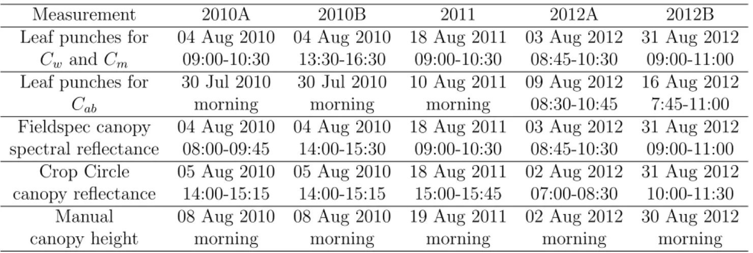
during the three field experiments (Table 1). Measurements were collected
186
in August during the cotton boll filling period. Collection times in 2011
187
and 2012 were focused in the morning hours after the 2010 data analysis
188
revealed larger differences in relative leaf water content between WW and
189
WL treatments earlier in the day (Carmo-Silva et al., 2012).
190
During each data collection outing, ground-based radiometric
measure-191
ments were collected over the selected Pima cultivars using a hand-held field
192
spectroradiometer (Fieldspec 3, Analytical Spectral Devices, Inc., Boulder,
193
CO, USA). Radiometric information was reported in 2151 narrow wavebands
from 350 to 2500 nm in 1 nm intervals. The instrument was equipped with
195
a 25◦ field-of-view fiber optic. To avoid soil background effects, a wand
con-196
structed from PVC tubing was used to position the fiber optic at a nadir
197
view angle approximately 0.25 m above the canopy. Because of the
proxim-198
ity of the sensor to the target, the methods are termed “proximal sensing”
199
as opposed to “remote sensing.” Frequent radiometric observations of a
cal-200
ibrated, 0.6 m2, 99% Spectralon panel (Labsphere, Inc., North Sutton, New
201
Hampshire) were used to characterize incoming solar radiation throughout
202
the data collection period. Because atmospheric absorption led to
insuffi-203
cient light in some wavebands, subsequent analyses of all spectral data used
204
1703 wavebands from 400 to 1350 nm, 1450 to 1770 nm, and 1970 to 2400
205
nm. Canopy reflectance factors in each waveband were computed as the
ra-206
tio of the canopy radiance over the corresponding time-interpolated value for
207
Spectralon panel radiance. Reflectance factors from six to twelve
radiomet-208
ric measurements over each experimental plot were averaged to estimate the
209
overall canopy spectral reflectance response. Variability in the number of
210
scans per plot was dependent on manual triggering of the spectroradiometer
211
while slowly walking through the field.
212
Simultaneously with canopy spectral reflectance measurements, two leaf
213
tissue samples were collected from two leaves in each plot with a 2 cm2
214
punch. Two leaf disks were collected per sample from one leaf at the top of
215
the canopy, sealed in a 3 × 4 cm2 pre-weighed ziplock bag, and stored on
216
ice in an insulated cooler. In the laboratory, the fresh weight of leaf samples
(mf) was measured on an electronic balance (AE 160, Mettler-Toledo, LLC,
218
Columbus, OH, USA). Leaf disks were then removed from the bags and oven
219
dried prior to dry weight (md) measurements. The leaf water thickness (Cw)
220
was calculated as the depth of water per unit leaf area (cm):
221
Cw = (mf −md)/(ρw×Als) (2)
where ρw is the density of water (1.0 g cm−3) andAls is the total area of the
222
leaf sample. The specific leaf mass (Cm, g cm−2) was also calculated:
223
Cm =md/Als (3)
Within two weeks of proximal hyperspectral measurements (Table 1),
224
additional leaf samples were collected for measurements of chlorophyll a+b
225
concentration (Cab). Two 0.3 cm2 leaf disks were obtained from each
exper-226
imental plot and stored at -80 ◦C. Using the method of Porra et al. (1989),
227
100% methanol (1 mL) was added to each sample for pigment extraction in
228
the dark at 4 ◦C for 48 h with mixing. A 200 µL sample of the supernatant
229
was collected for absorbance measurements at 652 nm (A652) and 665 nm
230
(A665), which were used to estimate Cab (µg cm−2):
231
Cab = (22.12A652+ 2.71A665)/Als (4)
Within one day of proximal hyperspectral measurements (Table 1), the
232
field-based high-throughput phenotyping system of Andrade-Sanchez et al.
(2014) was used to measure canopy reflectance, height, and temperature in
234
each experimental plot. Sensors were deployed on an open rider sprayer
235
(LeeAgro 3434 DL, LeeAgra, Lubbock, TX, USA) capable of sensing four
236
cotton rows simultaneously. Canopy reflectance was measured in 10 nm
wave-237
bands centered at 670, 720, and 820 nm using active multispectral
radiome-238
ters (Crop Circle ACS-470, Holland Scientific, Lincoln, NE, USA). Equation
239
1 was used to calculate NDVI from these data with ρ1 and ρ2 equal to
re-240
flectance values at 670 and 820 nm, respectively. Although canopy height was
241
measured by the phenotyping platform using sonar proximity sensors
(Pul-242
sar dB3, Pulsar Process Measurement Ltd, Malvern, UK), this study used
243
canopy height data measured manually using an electronic bar code scanner
244
with a coded measurement stick. Using the approach of Scotford and Miller
245
(2004), the NDVI from active radiometers and manual canopy height data
246
were used to calculate a compound canopy index (CCI), from which LAI was
247 estimated: 248 LAI = β×CCI = β c cmax h hmax (5)
where β is a constant, c and h are respectively the instantaneous canopy
249
cover and canopy height measurements, and cmax and hmax are respectively
250
the maximum cover and height expected during the growing season.
Co-251
located data to parameterize this calculation were collected during other
252
upland cotton experiments conducted at MAC from 2009 to 2013. Analysis
253
of these data led to values of 5.5, 87.9%, and 110.5 cm for β,cmax, andhmax,
respectively. The NDVI data from the active radiometers were used as a
255
direct estimate of cin Equation 5. Compared with 75 measurements from a
256
LAI meter (LAI-2200 Plant Canopy Analyzer, Li-Cor Biosciences, Lincoln,
257
NE, USA) and with LAI calculated using 75 measurements of leaf area from
258
biomass samples on an area meter (LAI-3100, Li-Cor Biosciences, Lincoln,
259
NE, USA), the index estimated LAI with a root mean squared error of 0.48
260
(15.9%).
261
2.3. Vegetation indices
262
Equation 1 was used to calculate three vegetation indices from the
proxi-263
mal hyperspectral data. The indices were selected based on their relevance to
264
monitor physiological stress in vegetation. A traditional broad-band NDVI
265
was calculated with ρ1 and ρ2 equal to the average spectral reflectance in
266
wavebands corresponding to the red (665 to 675 nm) and NIR (815 to 825
267
nm) filters used with the Crop Circle reflectance sensors onboard the
pheno-268
typing vehicle. The NDWI (Gao, 1996) was calculated with ρ1 and ρ2 equal
269
to the average spectral reflectance in wavebands corresponding to MODIS
270
Band 5 (1230 to 1250 nm) and Band 2 (841 to 876 nm), respectively.
Fi-271
nally, the PRI (Gamon et al., 1992) was calculated with ρ1 and ρ2 equal
272
to spectral reflectance at 531 nm and 570 nm, respectively. Linear
regres-273
sion models were developed to estimate Cw, Cm,Cab, and LAI using each of
274
these spectral indices. While these three indices were specifically highlighted,
275
Equation 1 was also used to calculate NDVI for all possible combinations of
276
the 1703 proximal hyperspectral wavebands.
2.4. PLSR modeling
278
PLSR was used to assess the relationships between each of the four
bio-279
physical variables and canopy spectral reflectance in 1703 wavebands. Thorp
280
et al. (2011) provided the details on the PLSR methodology used in the
281
present study. Briefly, if Y is an n×1 vector of responses (measured crop
282
phenotypes) and X is an n-observation by p-variable matrix of predictors
283
(hyperspectral reflectance measurements in pwavebands), PLSR aims to
de-284
compose X into a set of A orthogonal scores such that the covariance with
285
corresponding Y scores is maximized. The X-weight and Y-loading vectors
286
that result from the decomposition are used to estimate the vector of
regres-287
sion coefficients, βP LS, such that
288
Y =XβP LS + (6)
where is an n×1 vector of error terms.
289
The “pls” package (Mevik and Wehrens, 2007) within the R Project for
290
Statistical Computing (http://www.r-project.org) was used for PLSR in this
291
study. Four models were developed: one each for estimating Cw, Cm, Cab,
292
and LAI from the canopy spectral reflectance data. To choose the
appro-293
priate number of factors for each model (A from above), leave-one-out cross
294
validation was used to test model predictions for independent data, and scree
295
plots (not shown) provided the number of factors for which the root mean
296
squared error of cross validation (RMSECV) was minimized. The PLSR
297
models for Cw, Cm, Cab, and LAI were developed from the first five, eight,
eight, and ten factors, respectively.
299
2.5. PROSAIL simulations
300
The PROSAIL canopy reflectance model was developed by linking the
301
PROSPECT leaf optical properties model and the SAIL canopy bidirectional
302
reflectance model (Jacquemoud et al., 2009). PROSAIL uses 14 input
param-303
eters to define leaf pigment content, leaf water content, canopy architecture,
304
soil background reflectance, and illumination characteristics. Four of the
305
PROSAIL input parameters are the four biophysical variables measured in
306
this study: Cw,Cm,Cab, and LAI. In addition to Cab, other leaf pigment
pa-307
rameters include the carotenoid content (µg cm−2) and the brown pigment
308
content (unitless fraction from 0.0 to 1.0). Another leaf-scale parameter is
309
the leaf structural coefficient (N; unitless), defined as the number of leaf
310
mesophyll layers. In addition to LAI, canopy architecture is defined by the
311
average leaf inclination angle (θl; degrees). The background soil reflectance
312
parameter ranges from 0.0 for wet soils to 1.0 for dry soils. Specular
prop-313
erties of the canopy surface are characterized by the hot spot size parameter
314
(s; unitless fraction from 0.0 to 1.0). The skylight parameter (%) defines
315
the percentage of diffuse solar radiation. Illumination and viewer geometries
316
are characterized by the solar zenith angle (degrees), viewer zenith angle
317
(degrees), and relative solar and viewer azimuth angle (degrees). Based on
318
these inputs, the model calculates canopy bidirectional reflectance from 400
319
to 2500 nm in 1 nm increments.
320
PROSAIL has been developed in several programming languages. Initial
simulations were conducted using the Fortran version, which was compiled
322
using the “g95” Fortran compiler (http://www.g95.org) on a Linux operating
323
system. Later, PROSAIL for Python was deemed better for the simulation
324
analysis, because it encapsulated the Fortran code as an extension for the
325
Python programming language (http://www.python.org). This permitted
326
the model to be called from the Python command line and eliminated hard
327
disk access requirements for model input and output.
328
PROSAIL simulations were conducted on the “Stampede” supercomputer
329
at the Texas Advanced Computing Center (TACC), located at the University
330
of Texas in Austin. A single job submission was used to conduct 3.68 billion
331
PROSAIL simulations to test the effects of multiple parameter combinations
332
on simulated canopy spectral reflectance. Because proximal hyperspectral
333
measurements were collected in a total of 184 plots over all the field
experi-334
ments, 184 processing cores were requested such that the simulation analysis
335
could be explicitly conducted for the conditions of each experimental unit.
336
The maximum run time for a job submission on Stampede is 48 h. Thus, the
337
design objective was to conduct as many PROSAIL evaluations as possible
338
within the time limit.
339
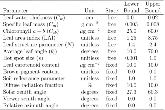
Seven parameters were adjusted during the PROSAIL simulation exercise
340
(Table 2). A Sobol quasirandom sequence algorithm for Python was used to
341
sample the parameter space. Although “less random” than a pseudorandom
342
number sequence, the approach tends to sample the parameter space “more
343
uniformly.” Another advantage is that the sequence is repeatable, so
cal parameter combinations could be tested for each experimental unit. For
345
Cw, Cm, Cab, and LAI, the lower and upper bounds were specified using the
346
range of measured values. Ranges for N,θl, and s were specified using
pub-347
lished values (Combal et al., 2003; Jacquemoud et al., 1995). Leaf carotenoid
348
content and brown pigment content were less sensitive parameters and were
349
fixed at 10.0 µg cm−2 and 0.0 (unitless), respectively. Because subsurface
350
drip irrigation was used, the soil surface was normally dry. Thus, the soil
351
reflectance parameter was fixed at 1.0 for all simulations. The fraction of
dif-352
fuse skylight was fixed at 10% based on observations of a shaded versus sunlit
353
Spectralon panel during the field study. By implementing the solar position
354
algorithm of Reda and Andreas (2004), solar zenith angles were calculated
355
from the timestamps of radiometric observations in the field. Observer zenith
356
and relative azimuth angles were both fixed at 0◦. This approach provided
357
an evaluation of 20 million combinations of seven PROSAIL parameters for
358
each of the 184 experimental units monitored during the field studies.
359
2.6. PROSAIL model inversion
360
Available storage allocation on Stampede became the limiting factor when
361
PROSAIL simulation results were initially written to the hard drive (i.e.,
362
1703 simulated reflectance values for 3.68 billion simulations would have
ex-363
ceeded the available storage allocation on Stampede). Thus, objective
func-364
tion evaluations were incorporated into the simulation exercise to reduce
stor-365
age requirements. Tested parameter sets were stored in a lookup table with
366
their corresponding objective function evaluations, including the root mean
squared error (RMSE) and the spectral angle (α) (Kruse et al., 1993) between
368
measured and simulated reflectance over all spectral wavebands (n= 1703):
369 RMSE = v u u t n X i=1 (Si−PROSAIL(P,C)i)2 (7) and 370 α= cos−1 Pn i=1Si×PROSAIL(P,C)i (Pn i=1S 2 i)0.5( Pn i=1PROSAIL(P,C) 2 i)0.5 (8)
whereSis the vector of measured canopy spectral reflectance and PROSAIL(P,C)
371
is the vector of simulated canopy spectral reflectance as a function of adjusted
372
parameters, P, and constant parameters,C. The main advantage of α is its
373
insensitivity to illumination, because Equation 8 incorporates only vector
374
direction and not vector length. This was considered advantageous because
375
proximal canopy spectral reflectance measurements were largely affected by
376
the fraction of sunlit versus shaded leaves in the instrument’s field of view.
377
Inversion of the PROSAIL model involved the identification of Pthat
mini-378
mized each of these objective functions for each experimental unit.
379
2.7. Statistics
380
For proximal hyperspectral sensing to be useful in field-based plant
phe-381
nomics, metrics obtained from the data must demonstrate differences among
382
the treatments imposed and be repeatable (i.e., heritable). Different
culti-383
vars can then be identified and selected as parents of breeding populations
384
for development of improved cultivars. Hierarchical linear mixed modeling
was used to assess differences among all data and metrics evaluated in this
386
study: field measurements, measured spectra, vegetation indices, PLSR
re-387
sults, and estimates from PROSAIL model inversion. Cultivar, water level,
388
and their interaction were modeled as fixed effects. Measurement date
(Ta-389
ble 1) and its interaction with both cultivar and water level were modeled
390
as random effects. Replicate plot, nested within measurement date and
wa-391
ter level, was also included as a random effect in the model. Hierarchical
392
tests required fitting random effects with 1) cultivar fixed effects alone, 2)
393
water level fixed effects alone, 3) both cultivar and water level fixed effects,
394
and 4) cultivar and water level fixed effects and their interaction. Likelihood
395
ratio tests were used to compare these hierarchical models, which showed
396
whether a given data set was different among cultivars, water levels, or their
397
interaction. Tukey’s multiple comparisons tests were also conducted to
iden-398
tify specific cultivars that were different for a given measurement. Statistics
399
were computed using the “lme4” package within the R Project for Statistical
400 Computing software. 401 3. Results 402 3.1. Field measurements 403
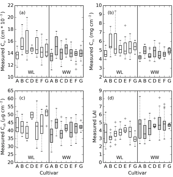
Measured values forCw, Cm, Cab, and LAI ranged from 0.01 to 0.02 cm,
404
0.003 to 0.009 g cm−2, 26.0 to 59.0 µg cm−2, and 1.7 to 8.3, respectively, 405
over all measurements collected (Fig. 1). Hierarchical linear mixed modeling
406
revealed differences in all four measured plant traits among cultivars (p <
407
0.01, Table 3). Differences in measured Cm and LAI were found among
the water levels (p < 0.05). The interaction of cultivar and water level
409
was significant for Cw and Cm (p < 0.05). Results for measured Cw and
410
Cm corroborate the results of Carmo-Silva et al. (2012), who conducted an
411
independent analysis using data from the 2010 season only. Typically, the
412
lowest and highest Cw were found for the Monseratt Sea Island and P62
413
cultivars, respectively (Fig. 1a), and Tukey tests confirmed Cw differences
414
between P62 and both Monseratt Sea Island and Pima S-6 for both WW
415
and WL treatments (p < 0.05). For WL conditions, Cm for Monseratt Sea
416
Island was less than four other cultivars: P62, 89590, PSI425, and Pima S-6
417
(p < 0.05). For WW conditions, Cm was lower for Monseratt Sea Island as
418
compared to P62 (p < 0.01, Fig. 1b). The Cab for P62 was greater than
419
both Monseratt Sea Island and 89590 (p <0.05) for WW conditions, but no
420
Cab differences were found among cultivars for the WL treatment (Fig. 1c).
421
With WW conditions, LAI for P62 was less than that for five other cultivars:
422
Monseratt Sea Island, Pima32, PSI425, Pima S-6, and Pima S-7 (p < 0.10,
423
Fig. 1d). Also, LAI for 89590 was less than that for Monseratt Sea Island,
424
Pima32, Pima S-6, and Pima S-7 (p <0.05). With WL conditions, LAI for
425
P62 was less than that for Monseratt Sea Island, Pima 32, and Pima S-6.
426
Based on measurements from five data sets, these results highlight the main
427
differences for measured traits among cultivars.
428
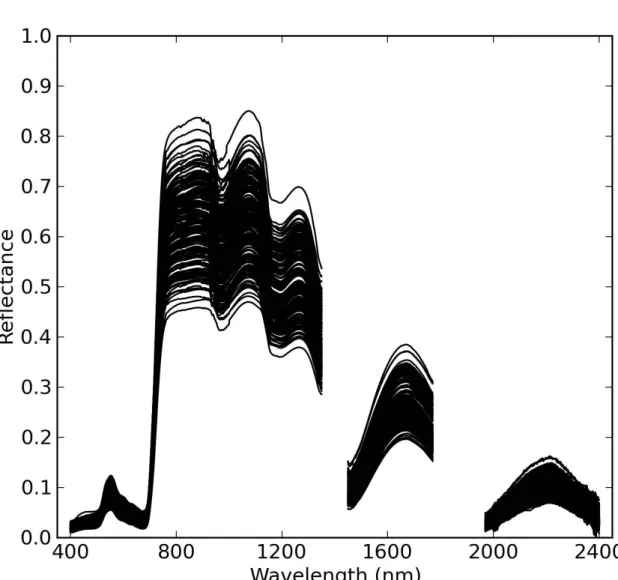
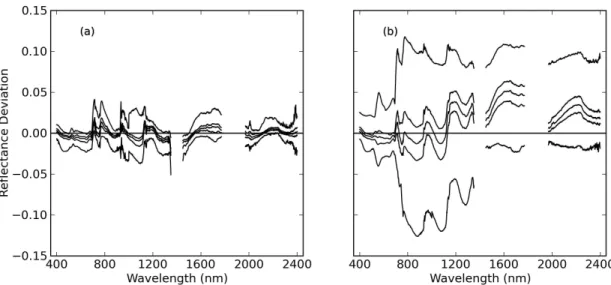
Proximal hyperspectral measurements of the cotton canopy followed
typ-429
ical patterns for spectral reflectance of vegetation (Fig. 2). Generally,
scat-430
tering of near-infrared radiation led to greater variability in reflectance from
760 to 1350 nm as compared to the visible (400 to 700 nm) and shortwave
432
infrared (1450 to 2400 nm) wavebands where chlorophyll and water,
respec-433
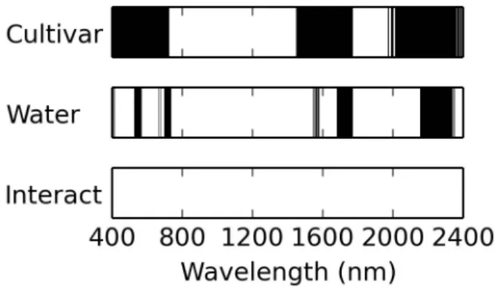
tively, absorb radiation. Results from hierarchical linear mixed modeling
434
demonstrated the wavebands with different reflectance values among water
435
levels and cultivars (p <0.05, Fig. 3). Among cultivars, spectral reflectance
436
differences were found in wavebands from 400 to 725 nm, 1470 to 1800 nm,
437
and 2000 to 2400 nm. Thus, reflectance in the entire visible portion of the
438
spectrum was different among cultivars, likely due to effects of radiation
ab-439
sorption by chlorophyll. Also, reflectance differences in two regions of the
440
shortwave infrared suggest effects of Cw or total plant water status. A fewer
441
number of wavebands demonstrated reflectance differences among water
lev-442
els, and four main regions were identified: 528 to 569 nm, 667 to 736 nm,
443
1681 to 1785 nm, and 2153 to 2353 nm. Wavebands around 550 nm
sug-444
gested that water level affected greenness of the canopy, while reflectance in
445
the far red and red edge bands were also affected. Reflectance differences
446
in the shortwave infrared bands again suggest effects of water level on plant
447
water status, as expected. Neither cultivar nor water level led to differences
448
in near-infrared reflectance, suggesting that other factors contributed to the
449
variability in those wavebands. There were also no significant cultivar by
450
water level interaction effects on reflectance.
451
3.2. Vegetation indices
452
Differences in broad-band NDVI from the spectroradiometer were found
453
for both the cultivar and water level treatments (Table 3), demonstrating
its robustness for proximal and remote sensing applications in agriculture.
455
Differences in broad-band NDWI were also found among cultivar and water
456
level treatments. Thus, the NDVI and NDWI could collectively provide
es-457
timates of both crop growth and water status. No differences in PRI were
458
found among cultivars or water levels. Also, unlike NDVI from the
spectro-459
radiometer, no differences in NDVI from the Crop Circle sensors were found
460
among cultivars. With a coefficient of determination (r2) of only 0.26 (not
461
shown), the relationship between Fieldspec NDVI and Crop Circle NDVI was
462
weak. This was likely related to different fields-of-view, measurement heights,
463
and light sources among the two sensors. Effects of soil background in the
464
instrument field-of-view was likely more of an issue for the tractor-mounted
465
Crop Circle than for the hand-held spectroradiometer.
466
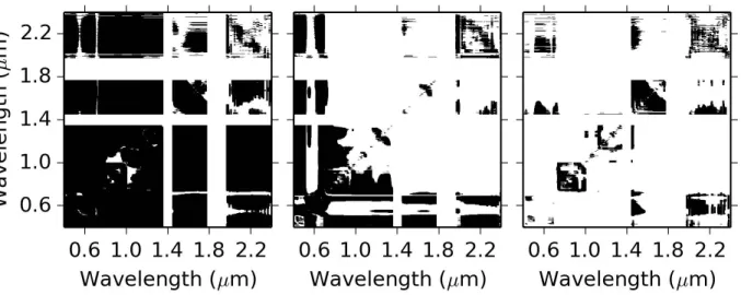
Many of the narrow-band NDVI calculations were different among
cul-467
tivars (p < 0.05, Fig. 4). When NDVI was computed using a waveband
468
from 400 to 1350 nm and any other waveband, the values often varied among
469
cultivars (p < 0.05). An exception was apparent when a red edge band was
470
used with any band greater than 1450 nm. Also, as shown in Table 3, the
471
wavebands used for PRI (i.e., 531 and 570 nm), which is itself a narrow-band
472
NDVI, did not lead to differences. Fewer differences among cultivars were
473
noted when NDVI was calculated using two wavebands greater than 1970 nm.
474
Fewer waveband combinations led to narrow-band NDVI differences among
475
water levels (Fig. 4). Notably, wavebands used for NDWI calculation (i.e.,
476
approximately 1240 and 858 nm) led to different narrow-band NDVI among
water levels (p < 0.05). Narrow-band NDVIs often did not demonstrate
sig-478
nificant cultivar by water level interactions, although significant interaction
479
effects were more common when two wavebands in either the near-infrared
480
(i.e., 730 to 1000 nm) or shortwave infrared (i.e., 1450 to 1770 nm) were used.
481
Linear regression models to estimate the measured crop phenotypes from
482
the vegetation indices were unfavorable compared to PLSR models, discussed
483
in the next section. None of the indices could estimate Cw, Cm, Cab, and
484
LAI with root mean squared errors better than 9.6%, 16.9%, 14.2%, and
485
28.8%, respectively. Cross-validated estimates from PLSR were better than
486
the estimates from linear relationships with vegetation indices. For LAI and
487
Cab, this result differed from that of Hansen and Schjoerring (2003), but
488
they compared narrow-band NDVI with PLSR and did not have spectral
489
reflectance measurements beyond 900 nm. Due to the linear nature of the
490
regression models, another concern is that the statistical results for traits
491
estimated in this way (not shown) were identical to that for the vegetation
492
index itself (Table 3). Thus, using linear regression to estimate traits from
493
vegetation indices did not provide any new information for hierarchical linear
494
mixed modeling.
495
3.3. PLSR modeling
496
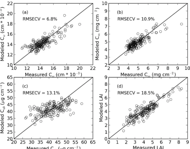
The PLSR models developed from 1703 wavebands of canopy spectral
497
reflectance estimated Cw, Cm, Cab, and LAI with RMSECV of 6.8%, 10.9%,
498
13.1%, and 18.5%, respectively (Fig. 5). Full spectrum data reduced root
499
mean squared errors between measured and modelled phenotypes as
pared to vegetation indices using reflectance in select wavebands.
Addition-501
ally, the PLSR results were cross-validated, so the PLSR models have been
502
properly tested with independent data.
503
Although the PLSR models provided better trait estimates than other
504
techniques, hierarchical linear mixed modeling results for PLSR estimates
505
were somewhat different than that for the field measurements (Table 3).
506
Whereas field-measured Cw, Cm, Cab, and LAI were all different among
cul-507
tivars, the PLSR estimates were different only for Cw and Cm (p < 0.01).
508
Also, whereas field measurements were different among water levels only for
509
Cm and LAI, the PLSR estimates for all four traits were different among
510
water levels (p < 0.05). Thus, the PLSR technique led to different trait
511
estimates among cultivars and water levels, but the results did not always
512
corroborate results for the field-measured traits.
513
3.4. PROSAIL simulations
514
Most biophysical models like PROSAIL were not originally designed with
515
high-performance computing in mind. Thus, efforts to use such models on
516
supercomputers demonstrate what is possible with modern computing
re-517
sources. Using the Fortran-compiled PROSAIL model, which required hard
518
disk access for model input and output, 40 million simulations were
com-519
pleted in 40.4 h for an average of 275 simulations per second. However, when
520
using the PROSAIL model compiled as a Python extension, 3.68 billion
sim-521
ulations were completed in 37.3 h for an average of 27,395 simulations per
522
second. Simulations could be multiplied 100 times by using a model that did
not require hard drive access.
524
Storage requirements were also a concern for the PROSAIL simulation
525
exercises. For trials with the Fortran-based PROSAIL model, the overall job
526
size was small enough to write simulated reflectance data in 1703 wavebands
527
to the hard disk. Using binary files to write reflectance data as 4-digit
in-528
tegers, simulated data for 40 million PROSAIL runs required 136.4 GB of
529
storage. Increasing the job size to 3.68 billion would thus increase storage
530
requirements to several TB, which exceeded allocation limits on Stampede.
531
Therefore, only the RMSE (Eq. 7) andα (Eq. 8) metrics were stored for the
532
larger job, which required only 36 GB. Decisions like these are central to the
533
design of supercomputing jobs for models like PROSAIL.
534
3.5. PROSAIL model inversion
535
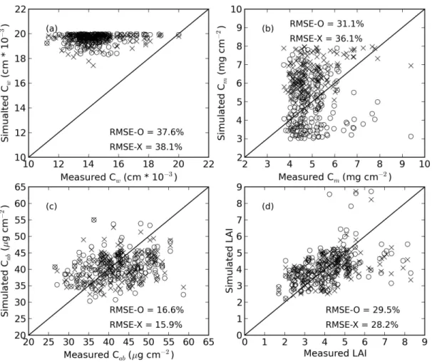
For the PROSAIL model inversion with the objective to minimize RMSE
536
between measured and simulated canopy spectral reflectance in 1703
wave-537
bands (Eq. 7), Cw, Cm, Cab, and LAI were estimated with RMSE of 37.6%,
538
31.1%, 16.6%, and 29.5%, respectively (Fig. 6). When the objective was to
539
minimizeαbetween measured and simulated canopy spectral reflectance (Eq.
540
8),Cw,Cm,Cab, and LAI were estimated with RMSE of 38.1%, 36.1%, 15.9%,
541
and 28.2%, respectively. Clearly, results from both objective functions were
542
inferior to that from PLSR models (Fig. 5). Discrepancies between measured
543
and simulated Cw suggested problems in how PROSAIL simulated effects of
544
leaf-level water content on canopy-level spectral reflectance (Fig. 6a).
In-545
versions with both objective functions resulted in higher Cw than measured,
and many optimumCw estimates were near the imposed upper bound of 0.02
547
cm (Table 2). This effect did not occur when reflectance in 501 wavebands
548
from 400 nm to 900 nm were used for PROSAIL model inversion. In this
549
case, RMSE between measured and simulated values dropped from 38% to
550
23% (not shown). Thus, discrepancies in the near-infrared wavebands above
551
900 nm and the shortwave infrared wavebands (discussed below) likely drove
552
the high error between simulated and measured Cw. This result highlights
553
the potential for model inversion outcomes to be affected by methodological
554
choices. Estimates of Cm based on minimum RMSE were often
underesti-555
mated, while Cm based on minimum α were overestimated for all but a few
556
cases (Fig. 6b). With high RMSE and low correlation between measured and
557
simulated values, Cw and Cm were the most difficult parameters to estimate
558
using PROSAIL model inversion.
559
Estimates of Cab from PROSAIL model inversion were more reasonable
560
(Fig. 6c), although the RMSEs between measured and simulated Cab were
561
still approximately 3% higher than that for the PLSR model. Estimates of
562
LAI were most problematic for values greater than 6.0 (Fig. 6d).
Measure-563
ment error is likely partially responsible for this result, because LAI
mea-564
surements were based on Crop Circle NDVI and canopy height according to
565
Equation 5. Some cultivars reached over 1.5 m in height, but Equation 5 was
566
parameterized using data from cotton with height less than 1.1 m. Thus,
567
the higher LAI “measurements” suffered from extrapolation issues. When
568
removing the LAI values above 6.0 from the calculation, the RMSE between
measured and simulated LAI was still above 22% which was 4% higher than
570
that for the PLSR model with all data included.
571
When the objective was to minimize RMSE between measured and
simu-572
lated canopy spectral reflectance, the resulting deviation between
PROSAIL-573
simulated and measured spectral reflectance was not greater than 0.05 at any
574
wavelength (Fig. 7a). In fact, simulated reflectance could often be optimized
575
to within 0.02 of measured reflectance for most wavelengths. This showed
576
that the inversion approach worked appropriately to find parameter values
577
that achieved the best fit between PROSAIL-simulated and measured canopy
578
spectral reflectance. When measured values for Cw, Cm, Cab, and LAI were
579
then substituted for the values obtained through PROSAIL model inversion,
580
the resulting deviations between PROSAIL-simulated and measured canopy
581
spectral reflectance (Fig. 7b) explain why PROSAIL model inversion had
582
problems producing accurate values for these parameters. Foremost, there
583
were greater positive deviations in reflectance from 1100 to 2400 nm. Thus,
584
the model overestimated reflectance in these wavebands when measured
pa-585
rameters were used. Also, there were greater deviations, up to 0.13, in the
586
near-infrared wavebands from 750 to 1350 nm. These results could indicate
587
errors in both measurement and modeling, and improvements could focus in
588
the mentioned waveband intervals.
589
Plotting the ranked RMSE and α statistics for the top 1% (200,000) of
590
PROSAIL evaluations provided insights on equifinality effects (Fig. 8).
Re-591
sults showed rapid departure from the minimum function evaluation within
the top 0.1% (20,000) of total model evaluations. Deviations from the
min-593
imum function evaluation were less variable for evaluations ranked greater
594
than 20,000, indicating greater equifinality effects with increasing evaluation
595
rank. The results suggest that model inversion identified a relatively small
596
fraction of parameter combinations with low RMSE andα statistics and that
597
equifinality was more problematic for parameter combinations other than
598
these. Parameter estimates forCw, Cm, Cab, and LAI that better agree with
599
measured values might be found within the top 20,000 evaluations. However,
600
equifinality renders the model inversion less useful above 20,000 evaluations.
601
Results also showed that the α statistic offered better separation from the
602
minimum function evaluation as compared to the RMSE statistic. Thus,
603
equifinality was less problematic for α than RMSE, but both statistics were
604
able to identify 0.1% of evaluated parameter combinations as top
candi-605
dates. Remaining issues include 1) understanding equifinality issues among
606
these top candidates and 2) addressing measurement and modeling errors to
607
insure estimated parameters are more accurate (Fig. 6).
608
Although PROSAIL model inversion estimated phenotypes with less
ac-609
curacy than other methods, many of the estimates differed among the water
610
level and cultivar treatments imposed during the field studies (Table 3).
Re-611
sults were often inconsistent between the objective functions used for model
612
inversion, which further highlighted the sensitivity of the inversion approach
613
to methodological choices. Generally, more traits were different when the
614
objective was to minimize α rather than RMSE (p < 0.05). Overall results
from PROSAIL model inversion were less accurate than that for PLSR
mod-616
els, but differences were nonetheless noted in parameter values estimated by
617
PROSAIL.
618
4. Discussion
619
While the differences among the Cw, Cm, Cab, and LAI measurements
620
were apparent and biologically meaningful (Table 3), the manual procedures
621
used to quantify these crop phenotypes were labor intensive and time
con-622
suming. Though practical here for 4 replications of 5 or even 25 cultivars,
623
obtaining these measurements for 1000 or 10000 cultivars would amplify
la-624
bor requirements greatly. Major bottlenecks include labor requirements for
625
collecting and processing leaf samples as well as time required for chemical
626
extraction of Cab and oven drying to obtain Cw and Cm. Thus, proximal or
627
remote sensing metrics that are able to discriminate these crop phenotypes
628
are essential for practical scaling of field-based plant phenomics experiments.
629
High-throughput approaches are needed for collection of field-based
prox-630
imal hyperspectral data. Time was the main limiting factor for the manual
631
approaches used in the present study. Six to twelve scans were collected in
632
each of 40 experimental plots in roughly 1.75 h. This provided data for only
633
one-fifth of the cotton cultivars grown in this relatively small study of 25
634
Pima lines. For larger studies with thousands of lines, high-throughput
ca-635
pability is a necessity. The averaged spectra for each experimental plot were
636
also highly variable in the near-infrared wavebands (Fig. 2), indicating
haps that more scans per plot were needed to ensure that spectral reflectance
638
of both sunlit and shaded portions of the canopy were adequately
character-639
ized. This is important because of the bidirectional reflectance distribution
640
function (BRDF) of the crop canopy, which defines how canopy reflectance
641
properties change with solar and viewer geometry. Because passive
spec-642
troradiometers use solar irradiance as the light source, a high-throughput
643
platform for such sensors must also collect data rapidly. This ensures that
644
BRDF effects on canopy spectral reflectance among experimental units are
645
minimal for a given data set. Use of an active field spectroradiometer with
646
its own light source could be another strategy for minimizing BRDF effects,
647
but the authors know of no such instrument for field-based proximal sensing
648
at this time. Finally, a high-throughput platform should enable canopy
spec-649
tral reflectance measurements from multiple view angles. This would permit
650
better characterization of BRDF effects and would provide more data to
651
constrain PROSAIL model inversion. A high-throughput sensing platform
652
capable of collecting much more than 12 spectral scans from a 8.8 m cotton
653
row at multiple view angles in a few seconds would be ideal for field-based
654
plant phenomics applications. To multiply efforts, sensing units with these
655
characteristics could be distributed along a tractor boom or gantry system
656
or perhaps mounted on a fleet of unmanned aerial systems.
657
To minimize BRDF impacts on canopy reflectance measurements, passive
658
reflectance sensing is often restricted to times near solar noon. In central
Ari-659
zona in August, this strategy provides two hours from 11:30 to 13:30 when
the solar zenith angle does not change by more than 5◦. Another strategy
661
is to maintain constant BRDF effects for spectral data collected over an
en-662
tire growing season. For cotton in Arizona, spectral measurements around
663
the time of a 45◦ solar zenith angle permits data collection with similar
664
BRDF characteristics from April to September. In the present study, the
665
goal was to collect spectral measurements concurrently with measurements
666
of Cw. Because prior studies demonstrated the dynamic diurnal response of
667
Cw and greater Cw variability among experimental treatments in the
morn-668
ing (Carmo-Silva et al., 2012), canopy spectral reflectance measurements
669
were primarily collected in the hours before and after solar noon (Table 1).
670
Concurrent spectral measurements with dynamic Cw was deemed more
im-671
portant than strict adherence to data collection at solar noon, although the
672
average solar zenith during spectral measurements was 42◦, similar to the 45◦
673
angle required for constant BRDF effects over a cotton season. Crop
pheno-674
types that undergo dynamic diurnal changes could require a departure from
675
traditional passive reflectance sensing techniques that restrict data collection
676
to solar noon. If the optimum time for monitoring a given phenotype occurs
677
while canopy spectral reflectance changes more rapidly due to BRDF effects,
678
efforts must focus on understanding these BRDF effects and on designing
679
sensors and sensing protocols that either characterize or minimize them. For
680
example, multiple view angles assist with BRDF characterization while rapid
681
spectral data collection minimizes illumination changes among experimental
682
units.
The PROSAIL model offers several advantages for field-based plant
phe-684
nomics, including its ability 1) to simulate BRDF effects on canopy spectral
685
reflectance and 2) to estimate phenotypes from canopy spectral reflectance
686
data alone. This study was limited to spectral reflectance measurements from
687
a nadir view angle, which likely limited efforts to estimate phenotypes using
688
PROSAIL model inversion. Data from multiple view angles should provide
689
more information to constrain PROSAIL, leading to better estimates. There
690
were also many methodological choices that impacted the PROSAIL model
691
inversion results, including the selected wavebands and the objective
func-692
tion. Future efforts should explore these issues in greater detail. For example,
693
with high-performance computing capabilities, a large database of PROSAIL
694
simulations could be generated and permanently stored. Multiple
measure-695
ment sets of a large mapping population over multiple years and locations
696
could then be inverted using the same database. Also, the data could be
697
used to develop confidence regions within the parameter space, which would
698
assist with parameter identification and equifinality issues.
699
As compared to PROSAIL model inversion, methods involving linear
re-700
gression on vegetation indices and PLSR on canopy spectral reflectance were
701
able to better quantify crop phenotypes. At this time, these methods remain
702
the most practical approach for crop phenotyping based on canopy
spec-703
tral reflectance. A main drawback of the regression approaches is that field
704
measurements of each phenotype are required for model fitting. A practical
705
approach for field phenomics may be to directly measure phenotypes for
lected experimental plots and to measure canopy spectral reflectance over all
707
plots using a high-throughput sensing platform. Data from plots with both
708
types of measurements could be used for building regression models, which
709
would subsequently be applied to estimate phenotypes for all experimental
710
units.
711
5. Conclusions
712
Proximal hyperspectral sensing offers a wealth of information for
char-713
acterizing reflectance from crop canopies and should be a fundamental
com-714
ponent of field-based plant phenomics programs. This study showed that
715
PLSR modeling was the most robust method for estimating Cw, Cm, Cab,
716
and LAI from canopy spectral reflectance data. Vegetation indices computed
717
from selected wavebands, including NDVI, NDWI, and PRI, were informative
718
but could not estimate phenotypes as well as PLSR. With improvements to
719
the PROSAIL model and ability to rapidly collect spectral reflectance data
720
from multiple view angles, model inversion for crop phenotyping may
be-721
come more practical. In the meantime, further investigations are needed to
722
improve PROSAIL model inversion strategies and to address related
equifi-723
nality issues. High-performance computing offers much potential for these
724
efforts and for overall advancements in the use of biophysical models for
725
agricultural applications.
6. Acknowledgments
727
The authors acknowledge the Texas Advanced Computing Center (TACC)
728
at the University of Texas at Austin for providing high-performance
comput-729
ing resources that contributed to the research results reported in this
pa-730
per (http://www.tacc.utexas.edu). This work is an outgrowth of an
iPlant-731
AgMIP modeling workshop at TACC in 2013. The iPlant Collaborative is
732
acknowledged for sponsoring the workshop and supporting travel for some
au-733
thors of this paper. Also, Kristen Cox, Joel Gilley, Suzette Maneely, Bradley
734
Roybal, and Sara Wyckoff are acknowledged for technical support. Doug
735
Hunsaker is acknowledged for assistance with irrigation scheduling. The
736
research was partially supported by National Science Foundation grant
DBI-737
1238187 and Cotton Incorporated.
738
Allen, R. G., Pereira, L. S., Raes, D., Smith, M., 1998. Crop
evapotranspi-739
ration: Guidelines for computing crop water requirements. FAO Irrigation
740
and Drainage Paper 56. Food and Agriculture Organization of the United
741
Nations, Rome, Italy.
742
Andrade-Sanchez, P., Gore, M. A., Heun, J. T., Thorp, K. R., Carmo-Silva,
743
A. E., French, A. N., Salvucci, M. E., White, J. W., 2014. Development and
744
evaluation of a field-based high-throughput phenotyping platform.
Func-745
tional Plant Biology 41 (1), 68–79.
746
Araus, J. L., Cairns, J. E., 2014. Field high-throughput phenotyping: The
747
new crop breeding frontier. Trends in Plant Science 19 (1), 52–61.
Babar, M. A., Van Ginkel, M., Klatt, A., Prasad, B., Reynolds, M. P.,
749
2006. The potential of using spectral reflectance indices to estimate yield
750
in wheat grown under reduced irrigation. Euphytica 150 (1-2), 155–172.
751
Bajwa, S. G., 2006. Modeling rice plant nitrogen effect on canopy reflectance
752
with partial least square regression (PLSR). Transactions of the ASABE
753
49 (1), 229–237.
754
Bannari, A., Morin, D., Bonn, F., Huete, A. R., 1995. A review of vegetation
755
indices. Remote Sensing Reviews 13 (1-2), 95–120.
756
Bolger, M. E., Weisshaar, B., Scholz, U., Stein, N., Usadel, B., Mayer, K.
757
F. X., 2014. Plant genome sequencing - applications for crop improvement.
758
Current Opinion in Biotechnology 26, 31–37.
759
Botha, E. J., Leblon, B., Zebarth, B., Watmough, J., 2007. Non-destructive
760
estimation of potato leaf chlorophyll from canopy hyperspectral reflectance
761
using the inverted PROSAIL model. International Journal of Applied
762
Earth Observation and Geoinformation 9 (4), 360–374.
763
Botha, E. J., Leblon, B., Zebarth, B. J., Watmough, J., 2010. Non-destructive
764
estimation of wheat leaf chlorophyll content from hyperspectral
measure-765
ments through analytical model inversion. International Journal of Remote
766
Sensing 31 (7), 1679–1697.
767
Carmo-Silva, A. E., Gore, M. A., Andrade Sanchez, P., French, A. N.,
Hun-768
saker, D. J., Salvucci, M. E., 2012. Decreased CO2 availability and
tivation of Rubisco limit photosynthesis in cotton plants under heat and
770
drought stress in the field. Environmental and Experimental Botany 83,
771
1–11.
772
Comar, A., Burger, P., De Solan, B., Baret, F., Daumard, F., Hanocq, J. F.,
773
2012. A semi-automatic system for high throughput phenotyping wheat
774
cultivars in-field conditions: Description and first results. Functional Plant
775
Biology 39 (11), 914–924.
776
Combal, B., Baret, F., Weiss, M., Trubuil, A., Mac, D., Pragnre, A.,
My-777
neni, R., Knyazikhin, Y., Wang, L., 2003. Retrieval of canopy biophysical
778
variables from bidirectional reflectance using prior information to solve the
779
ill-posed inverse problem. Remote Sensing of Environment 84 (1), 1–15.
780
Darvishzadeh, R., Matkan, A. A., Dashti Ahangar, A., 2012. Inversion of a
781
radiative transfer model for estimation of rice canopy chlorophyll content
782
using a lookup-table approach. IEEE Journal of Selected Topics in Applied
783
Earth Observations and Remote Sensing 5 (4), 1222–1230.
784
Fu, Y., Yang, G., Wang, J., Song, X., Feng, H., 2014. Winter wheat biomass
785
estimation based on spectral indices, band depth analysis and partial
786
least squares regression using hyperspectral measurements. Computers and
787
Electronics in Agriculture 100, 51–59.
788
Furbank, R., Tester, M., 2011. Phenomics - technologies to relieve the
phe-789
notyping bottleneck. Trends in Plant Science 16 (12), 635–644.
Gamon, J. A., Peuelas, J., Field, C. B., 1992. A narrow-waveband
spec-791
tral index that tracks diurnal changes in photosynthetic efficiency. Remote
792
Sensing of Environment 41 (1), 35–44.
793
Gao, B. C., 1996. NDWI - A normalized difference water index for remote
794
sensing of vegetation liquid water from space. Remote Sensing of
Environ-795
ment 58 (3), 257–266.
796
Gutierrez, M., Norton, R., Thorp, K. R., Wang, G., 2012. Association of
797
spectral reflectance indices with plant growth and lint yield in upland
798
cotton. Crop Science 52 (2), 849–857.
799
Hansen, P. M., Schjoerring, J. K., 2003. Reflectance measurement of canopy
800
biomass and nitrogen status in wheat crops using normalized difference
801
vegetation indices and partial least squares regression. Remote Sensing of
802
Environment 86 (4), 542–553.
803
Houle, D., Govindaraju, D. R., Omholt, S., 2010. Phenomics: The next
804
challenge. Nature Reviews Genetics 11 (12), 855–866.
805
Jacquemoud, S., 1993. Inversion of the PROSPECT + SAIL canopy
re-806
flectance model from AVIRIS equivalent spectra: Theoretical study.
Re-807
mote Sensing of Environment 44 (2-3), 281–292.
808
Jacquemoud, S., Baret, F., Andrieu, B., Danson, F. M., Jaggard, K.,
809
1995. Extraction of vegetation biophysical parameters by inversion of the