Interactive Volume Rendering on Standard PC Graphics Hardware
Using Multi-Textures and Multi-Stage Rasterization
C. Rezk-Salama∗ K. Engel† M. Bauer∗ G. Greiner∗ T. Ertl†
∗Computer Graphics Group, University of Erlangen, Germany
† Visualization and Interactive Systems Group, University of Stuttgart, Germany
Abstract
Interactive direct volume rendering has yet been restricted to high-end graphics workstations and special-purpose hard-ware, due to the large amount of trilinear interpolations, that are necessary to obtain high image quality. Implementations that use the 2D-texture capabilities of standard PC hard-ware, usually render object-aligned slices in order to substi-tute trilinear by bilinear interpolation. However the result-ing images often contain visual artifacts caused by the lack of spatial interpolation. In this paper we propose new render-ing techniques that significantly improve both performance and image quality of the 2D-texture based approach. We will show how multi-texturing capabilities of modern con-sumer PC graphics boards are exploited to enable interac-tive high quality volume visualization on low-cost hardware. Furthermore we demonstrate how multi-stage rasterization hardware can be used to efficiently render shaded isosurfaces and to compute diffuse illumination for semi-transparent vol-ume rendering at interactive frame rates.
Keywords: volume rendering, multi-textures, rasteriza-tion, PC hardware
1
Introduction
Interactive volume rendering has become an invaluable tech-nique to visualize 3D scalar data for a variety of applications in engineering, science and medicine. Due to the large num-ber of trilinear interpolations that must be processed in order to produce image results of high quality, the availability of direct volume rendering has yet been restricted to high-end workstations and special purpose graphics hardware. A brief outline of recent techniques is provided in Section 2.
Although there is a clear trend toward standard PC hard-ware as visualization platform [11], the application of in-teractive hardware-accelerated approaches is still limited. Volume rendering techniques that exploit the 2D-texturing hardware of PC graphics boards usually produce images that contain visual artifacts. The basic 2D-texture based approach is to decompose the volume into a set of object-aligned slices. The necessary trilinear interpolation can then be reduced to a bilinear interpolation which can be efficiently computed by standard texturing hardware. However, when zooming closely on a small detail inside the volume data, which is often done in medical applications, the missing tri-linear interpolation is strongly visible.
∗Lehrstuhl f¨ur Graphische Datenverarbeitung,
Am Weichselgarten 9, 91058 Erlangen, Germany, Email: [email protected]
†Abteilung f¨ur Visualisierung und Interaktive Systeme,
Breitwiesenstr. 20-22, 70565 Stuttgart, Germany, Email: [email protected]
Driven by the mass market of computer games and en-tertainment software, PC graphics accelerator boards have become more flexible and powerful. In Section 3, the capa-bilities of current PC rasterization hardware are described. Since our approaches exploits texturing and multi-stage rasterization, these features are explained in detail.
In Section 4 the basic ideas of texture based volume ren-dering are explained. As we will show in Section 5, the image quality of the 2D-texture based implementation can be greatly enhanced by performing real trilinear interpola-tion. This is achieved without loss in performance by in-terpolating intermediate slices using multi-textures. Section 6 describes how multi-textures can be further exploited to speed up rendering performance by mapping multiple slice images onto a single polygon. Section 7 adapts an algorithm for fast rendering of shaded isosurfaces to PC rasterization hardware and Section 8 describes methods to include local diffuse illumination for rendering semi-transparent volumes. Finally, in Section 9 an approach to interpolate slice images in arbitrary direction is discussed. Although the techniques described in this paper are aimed at an enhancement of the 2D-texture based approach, most of these methods are ready to be adapted to 3D-texturing hardware, which is very likely to be available on future graphics boards. In Section 10 the results of our study are evaluated by comparing performance and image quality of our solutions to standard 3D-texture based approaches of high-end graphics workstations. Sec-tion 11 briefly sums up the contents of our paper.
2
Related Work
There is a variety of different visualization approaches for scalar volumes in multiple application scenarios. Recent approaches are categorized into indirect methods, such as isosurface extraction [8, 5], and direct methods, that imme-diately display the voxel data. We will focus on interactive direct methods.
The basic idea of using object-aligned slices to substitute trilinear by bilinear interpolation was presented by Lacroute and Levoy [7], although the original implementation did not use texturing hardware. For the PC platform, Brady et al. [1] have presented a technique for interactive volume navi-gation based on 2D-texture mapping. More recently, Mueller et al. [10] used image based techniques to improve the per-formance of volume ray-casting.
The most important texture based approach was intro-duced by Cabral [2], who exploited the 3D-texture mapping capabilities of high-end graphics workstations. Westermann and Ertl [13] have significantly expanded this approach by introducing a fast direct multi-pass algorithm to display shaded isosurfaces. Based on their implementation, Meißner et al. [9] have provided a method to enable diffuse illumi-nation for semi-transparent volume rendering. However, in
this case multiple passes through the rasterization hardware led to a significant loss in rendering performance. Dachille et al.[3] have proposed an approach that uses 3D texture hard-ware interpolation and softhard-ware shading and classification.
In comparison to these techniques, we provide an en-hanced implementation of the fast isosurface algorithm in Section 7 using 2D-texturing hardware. In Section 8, we show how semi-transparent volumes can be rendered with ambient and diffuse illumination in a single-pass process us-ing the multi-stage rasterization hardware provided on PC graphics boards.
3
PC Graphics Hardware
For accelerated rendering, modern graphics boards provide a hardware implementation of the standard pipeline for dis-play traversal [6]. To produce images, geometric primitives (points, lines, triangles, etc.) are generated from the scene description and passed through this rendering pipeline. The process of image generation is then divided into three basic parts:
1. Thegeometry processingstep computes transformation and lighting for the geometric primitives.
2. Therasterization step then converts geometric primi-tives into pixel-values(fragments).
3. Finally,per-fragment operationslike blending or depth-test are performed before the fragments are written into the frame-buffer.
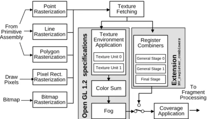
As mentioned above, rasterization denotes the process of converting geometric primitives into fragments, which co-incide with pixels in the resulting image. Each fragment contains information about color, opacity, depth and tex-ture values respectively. Recent PC graphics accelerator boards provide very flexible rasterization hardware, enabling advanced rendering techniques like per-pixel lighting or en-vironment mapping. The technique described in this paper efficiently exploit multi-texturing hardware. Multi-texturing is an optional extension introduced with OpenGL 1.2, allow-ing one polygon to be textured with image information ob-tained from multiple textures. OpenGL 1.2 specifies multi-texturing as a strict sequence of multi-texturing stages, which
al-Texture Fetching
Color Sum
Fog ApplicationCoverage Register Combiners Texture Environment Application Texture Unit 1 Texture Unit 0 To Fragment Processing Pixel Rect. Rasterization Bitmap Rasterization Polygon Rasterization Line Rasterization Point Rasterization From Primitive Assembly Draw Pixels Bitmap Open GL 1.2 specif ications Extension NV_register_combine rs General Stage 0 General Stage 1 Final Stage
Figure 1: Since the multi-texture model of OpenGL 1.2 turns out to be too limiting, NVidia’sGeForce 256processor pro-vides multi-stage register combiners that completely bypass the standard texturing unit.
lows to combine each texture with the results of the previous stage.
Although the basic idea of multi-texturing is represented by this specification, the concept of a static texture pipeline turns out to be not flexible enough for many desired ap-plications. Therefore recent PC graphics boards support multi-stage rasterization, which allows to explicitly control how color-, opacity- and texture-components are combined to form the resulting fragment. This allows rather complex calculations to be performed in a single rendering pass.
Although multiple rasterization stages are supported by PC graphics boards from different vendors, until now these features are optional extensions to the OpenGL standard and thus hardware-dependent. Since every manufacturer of graphics hardware defines its own extensions, we will restrict our description to graphics boards with NVidia’s GeForce 256 processor. The techniques described in Sections 5–8 were implemented using this multi-stage rasterization hard-ware.
To gain explicit control over per-fragment infor-mation, NVidia has provided the OpenGL extension
NV register combiners [12]. With this extension enabled,
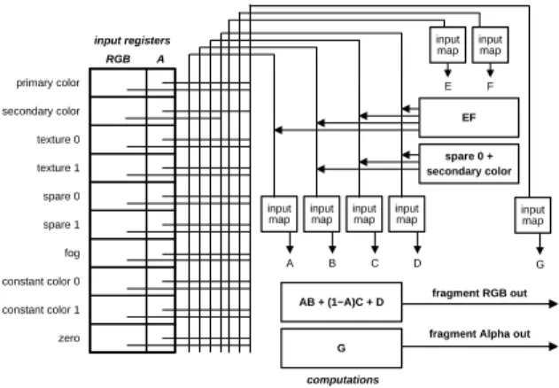
the standard OpenGL texturing units are completely by-passed and substituted by a register-based rasterization unit (see Fig. 1). This unit consist of two extremely flexible gen-eral rasterization stages and one final combiner stage. One general combiner stage is divided into an RGB-portion, dis-played in Figure 2 and a separate Alpha-portion, which is designed in a similar way, but can be programmed indepen-dently. not readable input
map inputmap inputmap inputmap
A B C D primary color secondary color texture 0 texture 1 spare 0 spare 1 fog constant color 0 constant color 1 zero primary color secondary color texture 0 texture 1 spare 0 spare 1 fog constant color 0 constant color 1 zero input registers output registers
RGB A RGB A computations scale and bias A B + C D −or− A B mux C D A B −or− A ● B C D −or− C ● D not writeable
Figure 2: The RGB-portion of the general combiner stage supports arbitrary register mappings and complex computa-tion like dot products and component-wise weighted sum.
In this hardware architecture per-fragment information is stored in a set of input registers (see Fig. 2). The contents of these registers can be arbitrarily mapped to the four vari-ables A, B, C and D. After combining these variables, i.e. by dot product (A•B) or component-wise weighted sum (AB+CD), the results are scaled and biased and are finally written to arbitrary output registers. The output registers of the first combiner stage are then the input registers for the next stage. An additional feature of this hardware is, that fixed point color components, which are usually clamped to a range of [0,1] can internally be expanded to a signed range [−1,1]. This allows also vector components to be stored in the color registers without the need to internally scale and bias them. The calculation of local diffuse illumination for the methods described in Section 7 and 8 is significantly simplified by this feature.
input map A B C D primary color secondary color texture 0 texture 1 spare 0 spare 1 fog constant color 0 constant color 1 zero input registers RGB A input map inputmap
input map inputmap
input
map inputmap
EF spare 0 + secondary color E F G AB + (1−A)C + D G computations fragment RGB out fragment Alpha out
Figure 3: The final combiner stage is used to compute the resulting fragment output for RGB and Alpha.
The output registers of the second general stage are com-bined by a final combiner stage displayed in Figure 3. The final stage only supports two output registers (RGB and Al-pha) and allows to compute AB+ (1−A)C+D for the RGB-portion. Additionally one of the variables A–D can be assigned to another intermediate component wise prod-uctE·F. After the multi-stage rasterization the standard OpenGL per-fragment operations, like depth test or alpha-blending are performed on the resulting fragment output from the final combiner stage. Note that this hardware also supports paletted textures, but the color-table lookup is performed before the interpolation, so the input
regis-terstexture 0andtexture 1already contain interpolated
RGBA values.
4
Texture Based Volume Rendering
In order to exploit texture hardware for volume rendering, the volume data set is represented by a stack of adjacent polygon slices. If 3D-textures (OpenGL 1.2) are supported by hardware, it is possible to render slices parallel to the image plane with respect to the current viewing direction (see Fig. 4 left). This means that if the viewing matrix changes, theseviewport-aligned slices must be recomputed. Since trilinear texture interpolation is supported by hard-ware, this can be done at interactive frame rate. In the final compositing step, the textured polygon slices are blended back-to-front onto the image plane, which results in a semi-transparent view of the volume. With this approach it is easy to enhance image quality just by increasing the num-ber of slices. However, in order to obtain equivalent repre-sentations of the volume data while changing the number of slices, opacity values must be adapted to the varying slice
Viewport-Aligned Slices Object-Aligned Slices Figure 4: Viewport-aligned slices(left)in comparison to ob-ject aligned slices(right)for a spinning volume object.
Figure 5: Visual artifacts are caused by the lack of trilin-ear interpolation(left) but can be successfully removed by inserting multiple intermediate slices(right).
distance. Although the correct scaling factor is a function of the opacity value, in most cases scaling the values linearly with a constant factor according to the slice distance is a visually adequate approximation.
In contrast, if hardware supports 2D-textures only, the slices are set parallel to the coordinate axes of the rectilinear data grid (object-alignedslices, Fig. 4(right)). This allows to substitute trilinear by bilinear interpolation. However, if the viewing direction changes by more that 90 degrees, the orientation of the slice normal must be changed. This requires to keep three copies of the data set in main mem-ory, one set of slices for each slicing direction respectively. The slices are rendered as planar polygons textured with the image information obtained from a 2D-texture map and blended onto the image plane. This is equivalent to an im-plicit decomposition of the viewing matrix into a 3D shear and a 2D image warp step as proposed in [7]. However, this factorization is not coded explicitly, since the decomposition is automatically performed by the OpenGL transformation matrix. Despite the high memory requirements, the ma-jor drawback of the 2D-texture based implementation is the missing spatial interpolation. As a result the images contain strong visual artifacts as displayed in Figure 5. To obtain correct visual results with this approach opacity values must be scaled according to the distance between two adjacent slices in direction of the viewing ray. Like in the 3D-texture based approach, scaling the values linearly with a constant factor as an approximation has lead to good visual results.
5
Multi-Texture Interpolation
In order to enhance the image quality of 2D-texture based volume rendering, an approach to remove the visual artifacts caused by the fixed number of slices is required. The idea to enable real trilinear interpolation is to compute interme-diate slices on the fly. The missing third interpolation step is then performed within the rasterization hardware using multi-textures.
Computing an intermediate slice Si+α can be described as a blending operation of two adjacent fixed slicesSi and
Si+1:
Si+α= (1−α)·Si+α·Si+1. (1)
With each slice image stored in a separate 2D-texture, bilin-ear interpolation is automatically performed by the texture unit. The third interpolation step is computed subsequently by blending the resulting two texels. As displayed in Fig-ure 6, the blending step can be computed by a single gen-eral combiner stage (see Sec. 3), if the fixed slices Si and
slice i slice (i +1) input registers RGB A texture 1 interpolation
factor α const color 1 texture 0 INVERT general combiner 0 A B C D A B + C D output register RGB A fragment A B C D final combiner A B + (1−A) C + D ZERO ZERO ZERO G Alpha portion: interpolated alpha RGB portion: interpolated color
Figure 6: Combiner setup for interpolation of intermediate slices.
Si+1 are specified as texture 0 and texture 1 using the
multi-texture extension. The combiner is setup to compute a component-wise weighted sumAB+CDwith the interpo-lation factorαstored in one of the constant color registers. The contents of this register is then mapped to input vari-ableAand at the same time inverted and mapped to vari-ableC. In the RGB-portion, variablesBandCare assigned
the RGB components oftexture 0andtexture 1
respec-tively. Analogously, the Alpha-portion interpolates between the alpha-components. For rendering semi-transparent vol-umes, the output of this first combiner stage is directly used for back-to-front alpha blending without any further modi-fication by the final combiner stage. Since multi-texture in-terpolation and combination is performed within one clock cycle of the graphics CPU, an intermediate slice is rendered at almost the same performance as a fixed single-textured slice. Of course multiple intermediate slices can be inserted this way without any increase in memory size. This appli-cation of multi-texturing greatly enhances image quality by removing visual artifacts as can be seen in Figure 5. Like in the 3D-texture based approach, opacity values must be adapted according to the new slice distance. This is approx-imated as usual by a constant linear scale factor.
d d d (0,0) (1,0) (1,1) texture polygon h w
corner view vector
v v v T1 T2 x y z w’ h’ d = slice distance w = slice width h = slice height w’= projected slice width h’= projected slice height x y z (s,t) (0,0) (1,0) (1,1) b = slice corner c = camera position slice polygon vertex
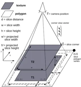
Figure 7: Correct texture mapping by calculating adapted texture coordinates for projected textures.
6
Performance Enhancement
In addition to the optimization of image quality described above, multi-texturing can be used to speed up rendering. In this section we are going to analyze an application of multi-textures for performance enhancement. The idea of this approach is to reduce the necessary number of triangles by mapping the textures of multiple slice images onto a single polygon.
If there arenindependent multi-texture units available, only everyn-th slice polygon is drawn, textured with the im-age information ofnconsecutive slice images. At first, the ntexture images are combined by multi-texturing hardware and the resulting fragment is blended into the frame buffer. If the combination ofntexture images can be computed in one clock cycle by the graphics CPU, rendering time will theoretically be reduced by a factor of 1/n. Additionally, frame buffer reads, which are necessary for back-to-front al-pha blending, are reduced by the same factor.
When mappingnslice images onto a single polygon, only the texture slice, which lies in the same plane of the slice polygon is drawn at the correct position due to perspective displacement of the other texture slices (see Fig. 13). In order to compensate this effect we increase width w and height hof a slice polygon by 2·d·(n−1) and adapt the texture coordinates to the new size. Although this technique can handle an arbitrary number of multi-texture units, for simplicity, we restrict our further considerations to only two textures.
Separate texture coordinates are calculated for each tex-ture image that is mapped onto the slice polygon. Observe that texture coordinates (s, t) of the slice image, which lies in the same plane as the polygon, are given by (1 +d
w,1 + d h) at the vertex marked in Figure 7. The texture coordinates of the subsequent slice images are adjusted by projecting the corners of the texture view-dependently onto the poly-gon. Figure 7 shows the adaptation of texture slice T2 to the slice polygon of texture slice T1. The view vector from camera position ~c to the corner of the slice~b is given by ~v= (vx, vy, vz)T =~c−~b. Then the displacement of the pro-jected slice in relation to the original corner position is given byd vx
−vy for thes-direction andd vz
−vy for thet-direction. According to this, the texture coordinates at the polygon vertex are given by
µ s0 t0 ¶ = µ 1 + d w0 +wd0·vx·vy 1 + d h0 +hd0··vvzy ¶ (2)
where w0 and h0 denote the width and height of the pro-jected texture. The texture coordinates of the other three vertices are calculated accordingly. Note that we obtain tex-ture coordinates greater than 1 and less than 0. Texel val-ues for coordinates outside the range of [0,1] should be set
input registers combinerfinal output register A B C A B + (1−A) C + D D RGB A RGB A slice i texture 0 texture 1 slice (i +1) RGB A G fragment ZERO general combiner 0 A B A B Alpha portion: A B C D C D A B RGB portion: INVERT INVERT INVERT
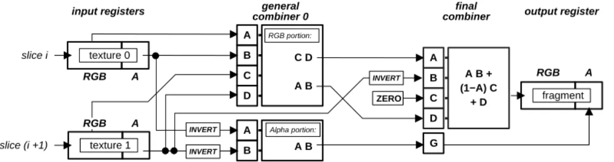
Figure 8: Combiner setup for correct blending of two slices
to zero. However, clamping textures to a fixed value (like
the SGIS texture edge clamp extension provided by SGI)
is currently not supported on GeForce 256 hardware. As a workaround, standard OpenGL texture clamping is used and the texture border must be initialized with zero values. The slice polygons are blended back-to-front into the frame buffer. Prior to this process thentexture maps must be combined correctly by the multi-texturing hardware. Let us proceed by considering the process of blending two sin-gle textured polygons into the frame buffer. During alpha blending, color values of the incoming fragment (the source) are combined with the color values at the corresponding frame buffer position (the destination) according to a speci-fied blend function.
In the following considerations the characterCindicates a R,GorBcolor component and the character A refers to an alpha value. Subscripts oft0 andt1indicate the texture
val-ues of the first and the second texture map. A subscript of dindicates a destination value and a subscriptsthe source value of an incoming fragment. Using the blending
func-tion glBlendFunc(GL SRC ALPHA,GL ONE MINUS SRC ALPHA)
for back-to-front rendering and theGL REPLACEtexture en-vironment, the resulting color value in the frame buffer after blending the first textured polygon amounts to
Cd0 =Ct0At0+Cd(1−At0). (3)
This color value is now used as the destination color when blending the second textured polygon.
Cd00 = Ct1At1+C
0
d(1−At1)
= Ct1At1+ (Ct0At0+Cd(1−At0))(1−At1)
= Ct1At1+Ct0At0(1−At1) +Cd(1−At0)(1−At1).
In order to get exactly this blending function during multi-texturing the register combiner have to be programmed as displayed in Fig. 8. The RGB-portion of general com-biner 0 is programmed to calculate Ct0At0 and Ct1At1.
The Alpha-portion of this combiner is used to compute (1−At0)(1−At1). The output of the RGB-portion are
routed into the final combiner stage which calculates the resulting RGB value
Cs=Ct0At0(1−At1) +Ct1At1. (4)
The result of the Alpha-portion is directly used as alpha value
As= (1−At0)(1−At1) (5)
of the output register. The resulting fragment is then blended into the frame buffer using the blending function
glBlendFunc(GL ONE,GL SRC ALPHA)resulting in
C00
d = Cs·1 +Cd·As
= Ct1At1+Ct0At0(1−At1) +Cd(1−At0)(1−At1).
Using this register combiner setup we obtain exactly the same blending results for multi-texturing as for rendering two separate polygons using single textures. A comparison of the image results can be seen in Figure 13.
7
Fast Shaded Isosurfaces
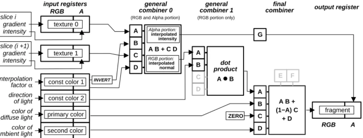
As mentioned in Section 2, Westermann and Ertl [13] have introduced an efficient algorithm that exploits rasterization hardware to display shaded isosurfaces. This method evalu-ates the equation of local illumination
I=Ia+Id·(~n•~l); (6) where~lis the direction of light and~nis the normal of the iso-surface which coincides with the volume gradient. IaandId are the intensities of ambient and diffuse light. At the core of the algorithm the vector components of the voxel gra-dients are stored in the RGB components of a 3D-texture image. Additionally the intensity values are stored in the alpha-component. The volume is then rendered into the frame buffer using the OpenGL alpha-test to display the specified isovalues only. In a second step, the frame buffer, that contains the voxel gradient coded in RGB components, is reinserted into the rasterization pipeline and the OpenGL color matrix is used to compute the dot-product with the light vector. This two-pass technique allows to efficiently render shaded isosurfaces at interactive frame rate. How-ever, the algorithm is restricted to a single light source and to monochrome display only.
Using multi-stage rasterization, this method can be effi-ciently adapted to PC hardware. The voxel gradient is com-puted as before and written into the RGB components of a set of 2D-textures that represent the volume. Analogously, the intensity is coded in the alpha-component. The regis-ter combiner are then programmed as displayed in Fig. 9. The first general combiner stage is applied as described in Section 5 to interpolate intermediate slices. The second gen-eral combiner is now enabled and computes the dot product A•B, where variableA is mapped to the RGB output of the first combiner stage (the interpolated gradient ~n) and variableB is mapped to the second constant color register, that contains the light vector~l. The alpha-component is not modified by the second combiner stage. Note that the gen-eral combiner stages support signed fixed point values, so
input registers
RGB A
interpolation
factor α const color 1
slice i texture 0 intensity gradient slice (i +1) texture 1 intensity gradient A B C D A B + C D INVERT color of diffuse light direction
of light const color 2
color of ambient light
primary color second color
general
combiner 0 combiner 1general
A B C D dot product A ● B output register final combiner RGB A fragment A B C A B + (1−A) C + D (RGB and Alpha portion) (RGB portion only)
RGB portion: interpolated normal Alpha portion: interpolated intensity D G E F ZERO
Figure 9: Combiner setup for fast rendering of shaded isosurfaces
there is no need to scale and bias the vector components to positive range.
As described in Section 3 the final combiner is capable of computingAB+ (1−A)C+D. When storing the color of diffuse and ambient light in the registers for primary and secondary color, the final combiner can be used to compute equation 6. Therefore variableAis assigned to primary color (Id) and is multiplied with variableBwhich is mapped to the dot product, computed by the RGB-portion of the second general combiner. VariableC is set to zero and variableD is mapped to secondary color (Ia).
Compared to the original work of Westermann and Ertl, our implementation is a single-pass rendering technique, since no copying of the frame buffer is required. Addition-ally, multi-stage rasterization allows the use of colored ambi-ent and diffuse light sources. As displayed in Figure 8, vari-ablesC andD are not used at the second combiner stage. The ability of the general combiner to compute a second dot productsC•D in parallel, can be used to compute lo-cal illumination for a second diffuse light source. However, the limiting factor is the available number of input registers, which are needed to store color and direction for the sec-ond light source. Unfortunately, it is not possible to write initial values to the two spare registers displayed in Fig. 2. Thus an additional colored diffuse light source can only be applied by sacrifice of either the trilinear interpolation or the specification of separate colors for ambient and diffuse light.
8
Shading for Semi-Transparent Volumes
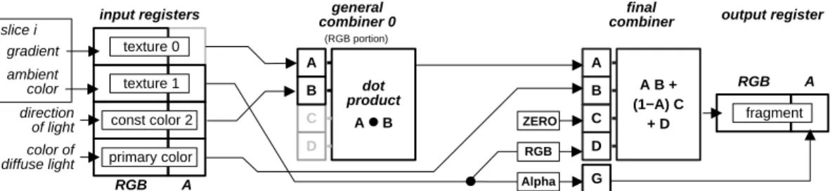
The fast algorithm to display isosurfaces directly leads to a shading technique for semi-transparent volume rendering. Using multi-stage rasterization hardware, there are two pos-sible methods to enable shading for semi-transparent vol-umes. The first approach is basically the same as the algo-rithm for shaded isosurfaces, with the exception that alpha-blending is used instead of the alpha-test. In this approach, however, there is no possibility to assign an ambient color for every data value independently, since the RGB channels are used as gradient vector and the alpha channel is used for opacity. As a result there is only a globally defined ambi-ent color, while normal vectors and opacity are defined for each voxel separately. Unfortunately, the hardware does not provide a component-wise color lookup table. Thus it is not possible for example to use the alpha-component as color index to specify ambient color for each voxel separately.
If specification of ambient color is desired on a per-voxel basis, this is also possible using current PC hardware, how-ever at the sacrifice of real trilinear interpolation. The basic idea of this approach is to use separate textures for gradient and color values. The first texture is an RGB texture, that contains the gradient information and the second texture contains the color and opacity information for every voxel. Note that the second texture can be a paletted texture of color indices, so the memory requirements are the same as for the isosurface algorithm (disregarding the memory allo-cated for the color table).
The register combiners for displaying shaded semi-transparent volumes are displayed in Fig. 10. In this sce-nario, the first combiner stage computes the dot product of the light vector (variableB) and the voxel gradient, obtained from the first texture (variableA). The final combiner sums up the ambient color stored in the second texture (variable D) and the product of diffuse color (B) with the dot product computed by the first combiner (variableA). Interpolation of intermediate slices is not possible, since current hardware only supports two input textures at a time. However, as de-scribed in Section 7, variablesCandDof the first combiner stage can now be used to compute diffuse illumination for a second colored light source, since the input registers for secondary color and constant color 1 are unused.
Despite the lack of real trilinear interpolation, this ap-proach has several advantages compared to the implementa-tion proposed in [9]. Since the dot product is directly sup-ported by the hardware, illumination is computed in a single-pass rendering process, and thus interactive frame rates are achieved. Additionally no large-scale workaround is required to allow for signed vector components, since they are also supported by hardware. The main drawback is that the image quality is limited, due to the missing real trilinear interpolation. However we are confident that future hard-ware will provide a higher number of texturing units or even 3D-texturing capabilities.
9
Interpolation of Arbitrary Slices
In addition to direct volume rendering, many applications require to interpolate slice images of the volume data set in arbitrary direction. In medicine this is usually referred to as multi-planar reformatting (MPR).
An interesting 2D-texture based technique to render ar-bitrary slices was introduced in [4] and is easily adapted to
texture 1 input registers RGB A slice i texture 0 ambient color gradient general
combiner 0 combinerfinal output register
(RGB portion)
color of diffuse light
direction
of light const color 2
primary color A B C D dot product A ● B A B C A B + (1−A) C + D D ZERO RGB RGB A fragment G Alpha
Figure 10: Combiner setup for rendering semi-transparent volumes with local diffuse illumination
calculate
cross−section cut polygon into stripes specify alpha values multi−textureapply
Figure 11: Rendering procedure to interpolate slice images in arbitrary direction.
multi-texturing hardware. The basic idea of this algorithm is displayed in Fig. 11. At first the cross-section of the slic-ing plane with the boundslic-ing box of the volume is calculated. The resulting intersection polygon is then cut into a set of polygon strips at the intersection line with the object-aligned texture slices. Subsequently for each of these polygon strips the image information is obtained by interpolating the two adjacent texture images. This is achieved by specification of alpha values for the polygon vertices. In this case an alpha value of 0 indicates that the corresponding vertex should be textured with the image information from the first texture. Accordingly, if a value of 1 is specified the second texture image is applied. Within the polygon, Gouraud shading is used to interpolate between the alpha values specified at the polygon vertices. The interpolation between the two tex-ture images is finally performed by the register combiners as displayed in Figure 12. In this scenario, general combiner 0 is programmed to blend both textures (mapped to vari-ables A and C) using the primary color alpha (mapped to variable B and inverted to variable D). As mentioned above, primary alpha is interpolated between the values specified at the vertices. slice i slice (i +1) input registers RGB A texture 1 interpolation
factor α primary color
texture 0 INVERT general combiner 0 A B C D A B + C D Alpha portion: interpolated alpha RGB portion: interpolated color
Figure 12: Combiner setup for interpolation of arbitrary slice images
Although, the described technique is usually applied to interpolate single slice images, it is potentially applicable for volume rendering with viewport-aligned slices. However,
the significant computational overhead for intersection cal-culation in combination with the large number of texture binding operations results in a poor rendering performance. Using viewport aligned slices only 5—8 frames per seconds were achieved for a small data set of size 643.
10
Results
The presented algorithms were implemented on Windows
NT platform on a standard PC (AGP 2×) with single
500 MHz Intel Pentium III CPU and a graphics board with
NVidia GeForce 256 processor and 32 MB of double data
RAM.
Figure 14(A) shows the comparison of the standard single-texture based approach with our method to enhance per-formance using multi-textures (Section 6). When multi-texturing is enabled, the number of polygons to be rendered is reduced by a factor of 2. Theoretically this should results in a speedup of rendering performance also by a factor of 2. However, as displayed in Figure 14(A) we only achieve a factor of 1.8. This might be an effect of the limited memory bandwidth. Although we only render half the polygons, the complete texture information must be accessed during one render pass.
A. Single and Multi−Textures 128x128x64 256x256x128 256x256x256 0 5 10 15 20 25 30 35 40 45 50 55 54.9 29.7 22.2 12.3 7.8 4.3 0 5 10 15 20 25 22.5 4.1 2.0
B. Shaded Semi−Transparent Volumes 128x128x64
256x256x128 256x256x256
dual texture single texture
frames per second
frames per second Figure 14: Performance measurement using a viewport size of 600×600 pixels: (A) Frame rates of single- versus multi-texture rendering. (B) Frame rates of shaded direct volume rendering
The visual artifacts displayed in Figure 13 are completely removed by adjustment of the texture coordinates and cor-rect blending computation using the register combiners. The computational overhead to calculate correct texture coordi-nates does not significantly influence the frame rate. Turn-ing this calculation off only increases the performance by 0.2 frames per second for a data set of moderate size. However due to the mapping of texture slices at incorrect positions in
Figure 13: Right: Image results of single-texture based approach. Middle: Multi-texture based approach without correction generates visual artifacts. Left: The artifacts are successfully removed by correction of texture coordinates.
3D, problems may occur when using clipping planes. Coping with these problems will be focused on in the future.
The usage of multi-texturing does significantly increase performance of texture based volume rendering without any loss in image quality compared to the standard 2D-texture based approach. The different rendering algorithms
pre-36.7 Onyx2 Base Reality A. CTA Aneurysm (128 x 128 x 64) 0 5 10 15 20 25 30 35 29.7 3.1 18.5 13.4 10.2 8.9 7.3 2.3
direct volume rendering
shaded isosurface 16.7 13.7 4.2 5.6 1.5 4.1 8.9 GeForce 256 100% 200% 300% 1000% 100% 200% 300% 1000% 40 0 1 2 3 4 5 6 7 8 100% 200% 300% 1000% 100% 200% 300% 1000%
direct volume rendering
shaded isosurface
C. MR Head (256 x 256 x 256) GeForce 256 Onyx2 Base Reality 4.3 7.3 2.3 1.3 0.4 0.8 2.7 3.9 1.7 4.0 1.7 2.2 1.5 1.5 0.4 0.5 14 Onyx2 Base Reality B. Engine Block (256 x 256 x 128) 2 4 6 8 10 12 0 100% 200% 300% 1000% 100% 200% 300% 1000% shaded isosurface direct volume rendering
GeForce 256 12.4 6.7 6.8 4.0 3.7 2.7 1.4 1.3 4.0 3.9 3.6 2.1 3.0 1.6 0.8 0.5 14 frames per second
frames per second
frames per second
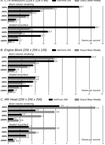
Figure 15: Frame rates of the GeForce 256
implementa-tion in comparison to the 3D-texture soluimplementa-tion on SGI Onyx2 BaseReality (viewport 600×600)
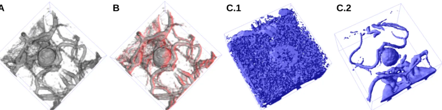
sented in this paper were evaluated using volume data sets of different resolution. Figure 16 displays a computed tomog-raphy angiogtomog-raphy (CTA) data set showing an intracranial aneurysm. Image A displays the results of direct volume rendering without illumination. In image B a colored diffuse light source has been added using the approach described in Section 8. The achieved frame rates for shading semi-transparent volumes are displayed in Figure 14(B). Com-paring these values to the performance of the 3D-texture based multi-pass solution presented in [9] clearly demon-strates the benefits of multi-stage rasterization. The results of the isosurface algorithm (Section 7) are displayed in Fig-ures 16 (C.1) and (C.2) for different isovalues. Note that we are able to interactively display isosurfaces in noisy data (C.1), where polygon-based algorithms are bound to fail due to the resulting extremely high number of triangles. In Fig-ure 15(A) performance of the presented multi-textFig-ure im-plementation on NVidiaGeForce 256hardware is compared to 3D-texture based volume rendering performed on an SGI Onyx2 with BaseReality graphics hardware and 64 MB of texture memory. For the CTA data set of size 128×128×64,
theGeForce 256implementation reaches significantly higher
frame rates, even if the data set is extremely super-sampled by increasing the number of slices from 100% to 1000%. It is also remarkable that on GeForce 256isosurfaces display is significantly faster than direct volume rendering. Obvi-ously reading the frame-buffer, which is required for alpha-blending semi-transparent slices, but not for the isosurface display, is rather expensive onGeForcehardware. Figure 17 displays the image results of our implementation for the engine block data set of size 256×256×128. Image A was generated using direct volume rendering with 300%
super-sampling and without illumination. Shaded
semi-transparent representations are displayed in Image B.1 and B.2 for different opacity settings. Image C.1 and C.2 show the results of fast isosurface rendering for different isovalues using a blue ambient color and a single diffuse white light source. Image C.3 demonstrates the application of two light sources. The second light source was enabled as described in Section 7 by sacrifice of color specification for diffuse light sources. As displayed in Figure 15(B) theGeForce imple-mentation still achieves significantly higher performance for both direct volume rendering and isosurface display. How-ever, due to the higher memory requirements for gradient textures, the frame rate for isosurface rendering is now sig-nificantly lower that for semi-transparent display. In
con-trast to the color-index texture used for semi-transparent rendering, the RGBA texture for isosurface display does not fit entirely into graphics memory and is thus swapped into main memory via AGP (2×) bus.
Finally, for the MR head (Fig. 18(A)) of resolution 256× 256×256, the Onyx2 clearly dominates in rendering per-formance as displayed in Figure 15(C). The limited mem-ory bandwidth of the AGP port is evident when comparing the frame rates for isosurface display at 100% and 200%. Although the number of textured slices has increased by a factor of 2, the achieved frame rate remains the same. Fig-ure 18(B) displays image results for a large CT data set of size 512×512×106, which were generated at approximately 1 frame per second onGeForce 256hardware.
As we have demonstrated the multi-texture based volume rendering onGeForce 256hardware has proved superior for displaying volume data sets of moderate size. Using multi-texture interpolation, the resulting images quality is equiv-alent to 3D-texture based solutions. The only drawback of
GeForce 256hardware is the lack of post-interpolative color
lookup tables, which are necessary for high precision transfer functions.
In order to build a scalable volume rendering application, the presented techniques for performance and quality en-hancement can be combined. While user interaction events are scheduled in the event queue, performance optimization is used to provide high frame rate. In consequence, if the event queue is empty, image quality is optimized. Current PC graphics hardware only supports two independent multi-texturing units. However, performance of the presented al-gorithms will greatly benefit from a higher number of avail-able textures. Additionally, with the exception of multi-texture interpolation, all presented methods are ready to be extended to 3D-textures, when they are finally supported by future graphics boards.
11
Conclusion
On the basis of standard 2D-texture based volume rendering we have introduced several advanced rendering techniques, that exploit rasterization hardware of PC graphics boards in order to significantly improve both performance and image quality. The presented approaches are based on the multi-texturing and the multi-stage rasterization capabilities of NVidia’sGeForce 256processor. The resulting image qual-ity is equivalent to 3D-texture based solutions provided by high-end graphics workstations. We have also shown that for volume data sets of moderate size PC graphics hardware is significantly faster than high-end systems. Furthermore, advanced algorithms like fast isosurface display or shaded volume rendering are efficiently adapted to the PC platform. Since only low-cost hardware is required, the presented ap-proaches significantly contribute to the availability of inter-active direct volume rendering in practice.
12
Acknowledgments
We thank John Spitzer and NVidia for providing information and image material about theGeForce 256hardware.
References
[1] M. Brady, K. Jung, Nguyen HT, and T. Nguyen. Two-Phase Perspective Ray Casting for Interactive Volume Navigation. InVisualization ’97, 1997.
[2] B. Cabral, N. Cam, and J. Foran. Accelerated Vol-ume Rendering and Tomographic Reconstruction Using Texture Mapping Hardware.ACM Symp. on Vol. Vis., 1994.
[3] F. Dachille, K. Kreeger, B. Chen, I. Bitter, and A.
Kauf-man. High-Quality Volume Rendering Using
Tex-ture Mapping Hardware. InSIGGRAPH Eurographics
Graphics Hardware Workshop, 1998.
[4] G. Eckel.OpenGL Volumizer Programmer’s Guide. SGI Developer Bookshelf, 1998.
[5] K. Engel, R. Westermann, and T. Ertl. Isosurface ex-traction techniques for web-based volume visualization. InVisualization ’99, 1999.
[6] J. Foley, A. van Dam, S. Feiner, and J. Hughes.
Computer Graphics, Principle And Practice.
Addison-Weseley, 1993.
[7] P. Lacroute and M. Levoy. Fast Volume Rendering Us-ing a Shear–Warp Factorization of the ViewUs-ing Trans-form . Comp. Graphics, 28(4), 1994.
[8] W.E. Lorensen and H.E. Cline. Marching Cubes: A High Resolution 3D Surface Reconstruction Algorithm.
Comp. Graphics, 21(4), 1996.
[9] M. Meißner, U. Hoffmann, and W Straßer. Enabling Classification and Shading for 3D Texture Based
Vol-ume Rendering Using OpenGL and Extensions. In
Vi-sualization ’99, 1999.
[10] K. Mueller, N. Shareef, J. Huang, and Crawfis. R. IBR-Assisted Volume Rendering. InVisualization 1999 Late
Breaking Hot Topics, 1999.
[11] H. Pfister. Why the PC will be the most pervasive visualization platform in 2001. In Visualization ’99, 1999.
[12] J. Spitzer. GeForce 256 and RIVA TNT Combiners. http://www.nvidia.com/Developer.
[13] R. Westermann and T. Ertl. Efficiently Using Graphics Hardware in Volume Rendering Applications. InProc.
A
B
C.1
C.2
Figure 16: CTA aneurysm data set (1282×64): (A) direct volume rendering without illumination, (B) direct volume rendering
with red diffuse light source, (C) shaded isosurface for different isovalues.
A B.1 B.2
C.1 C.2 C.3
Figure 17: Engine Block (2562×128): direct volume rendering without illumination (A), shaded (B.1), shaded with lower
opacity (B.2) and shaded isosurface (C.1) and (C.2) with diffuse white light source and with two white light sources (C.3)
A B.2 B.2