Visual navigation of a mobile robot with laser-based collision avoidance

Visual Navigation of a Mobile Robot

with Laser-based Collision Avoidance

Andrea Cherubini∗1,2_{and François Chaumette}†1

1_{INRIA Rennes - Bretagne Atlantique, IRISA, Campus de Beaulieu 35042, Rennes, France} 2_{LIRMM - Université de Montpellier 2 CNRS, 161 Rue Ada, 34392 Montpellier, France}

August 19, 2012

Abstract

In this paper, we propose and validate a framework for visual navigation with collision avoidance for a wheeled mobile robot. Visual navigation consists of following a path, represented as an ordered set of key images, which have been acquired by an on-board camera in a teaching phase. While following such path, the robot is able to avoid obstacles which were not present during teaching, and which are sensed by an on-board range scanner. Our control scheme guarantees that obstacle avoidance and navigation are achieved simultaneously. In fact, in the presence of obstacles, the camera pan angle is actuated to maintain scene visibility while the robot circumnavigates the obstacle. The risk of collision and the eventual avoiding behaviour are determined using a tentacle-based approach. The framework can also deal with unavoidable obstacles, which make the robot decelerate and eventually stop. Simulated and real experiments show that with our method, the vehicle can navigate along a visual path while avoiding collisions.

Keywords: Vision-based Navigation, Visual Servoing, Collision Avoidance, Integration of vision with other sensors.

∗

Andrea.Cherubini@lirmm.fr †

1

Introduction

A great amount of robotics research focuses on vehicle guidance, with the ultimate goal of

automati-2

cally reproducing the tasks usually performed by human drivers [Buehler et al. 2008, Zhang et al. 2008,

3

Nunes et al. 2009, Broggi et al. 2010]. In many recent works, information from visual sensors is used for

lo-4

calization [Guerrero et al. 2008, Scaramuzza and Siegwart 2008] or for navigation [Bonin-Font et al. 2008,

5

López-Nicolás et al. 2010]. In the case of autonomous navigation, an important task is obstacle

avoid-6

ance, which consists of either generating a collision-free trajectory to the goal [Minguez et al. 2008], or

7

decelerating to prevent collision when bypassing is impossible [Wada et al. 2009]. Most obstacle avoidance

8

techniques, particularly those that use motion planning [Latombe 1991], rely on the knowledge of a global

9

and accurate map of the environment and obstacles.

10

Instead of utilizing such a global model of the environment, which would infringe the perception

11

to action paradigm [Sciavicco and Siciliano 2000], we propose a framework for obstacle avoidance with

12

simultaneous execution of a visual servoing task [Chaumette and Hutchinson 2006]. Visual servoing is

13

a well known method that uses vision data directly in the control loop, and that has been applied on

14

mobile robots in many works [Mariottini et al. 2007, Becerra et al. 2011, López-Nicolás and Sagüés 2011,

15

Allibert et al. 2008]. For example, in [Mariottini et al. 2007] the epipolar geometry is exploited to drive a

16

nonholonomic robot to a desired configuration. A similar approach is presented in [Becerra et al. 2011],

17

where the singularities are dealt with more efficiently. The same authors achieve vision-based pose

sta-18

bilization using a state observer in [López-Nicolás and Sagüés 2011]. Trajectory tracking is tackled in

19

[Allibert et al. 2008] by integrating differential flatness and predictive control.

20

The visual task that we focus on is appearance-based navigation, which has been the target of our

21

research in [Šegvi´c et al. 2008, Cherubini et al. 2009, Diosi et al. 2011]. In the framework that we have

de-22

veloped in the past1, the path is a topological graph, represented by a database of ordered key images. In

23

contrast with other similar approaches, such as [Booij et al. 2007], our graph does not contain forks.

Further-24

more, as opposed to [Royer et al. 2007, Goedemé et al. 2007, Zhang and Kleeman 2009, Fontanelli et al. 2009,

25

Courbon et al. 2009], we do not use the robot pose for navigating along the path. Instead, our task is purely

26

image-based (as in [Becerra et al. 2010]), and it is divided into a series of subtasks, each consisting of driving

27

the robot towards the next key image in the database. More importantly, to our knowledge, appearance-based

28

navigation frameworks have never been extended to take into account obstacles.

29

1

Obstacle avoidance has been integrated in many model-based navigation schemes. In [Yan et al. 2003],

1

a range finder and monocular vision enable navigation in an office environment. The desired trajectory

2

is deformed to avoid sensed obstacles in [Lamiraux et al. 2004]. The authors of [Ohya et al. 2008] use a

3

model-based vision system with retroactive position correction. Simultaneous obstacle avoidance and path

4

following are presented in [Lapierre et al. 2007], where the geometry of the path (a curve on the ground)

5

is perfectly known. In [Lee et al. 2010], obstacles are circumnavigated while following a path; the radius

6

of the obstacles (assumed cylindrical) is known a priori. In practice, all these methods are based on the

7

environment 3D model, including, for example, walls and doors, or on the path geometry. In contrast, we

8

propose a navigation scheme which does not require neither the environment nor the obstacle model.

9

One of the most common techniques for model-free obstacle avoidance is the potential field method,

10

originally introduced in [Khatib 1985]. The gap between global path planning and real-time sensor-based

11

control has been closed with the elastic band [Quinlan and Khatib 1993], a deformable collision-free path,

12

whose initial shape is generated by a planner, and then deformed in real time, according to the sensed data.

13

Similarly, in [Bonnafous et al. 2001, Von Hundelshausen et al. 2008], a set of trajectories (arcs of circles or

14

“tentacles”) is evaluated for navigating. However, in [Bonnafous et al. 2001], a sophisticated probabilistic

15

elevation map is used, and the selection of the optimal tentacle is based on its risk and interest, which both

16

require accurate pose estimation. Similarly, in [Von Hundelshausen et al. 2008], the trajectory computation

17

relies on GPS way points, hence - once more - on the robot pose.

18

Here, we focus on this problem: a wheeled vehicle, equipped with an actuated pinhole camera and with

19

a forward-looking range scanner, must follow a visual path represented by key images, without colliding

20

with the ground obstacles. The camera detects the features required for navigating, while the scanner senses

21

the obstacles (in contrast with other works, such as [Kato et al. 2002], only one sensor is used to detect the

22

obstacles). In this sense, our work is similar to [Folio and Cadenat 2006], where redundancy enables reactive

23

obstacle avoidance, without requiring any 3D model. A robot is redundant when it has more DOFs than those

24

required for the primary task; then, a secondary task can also be executed. In [Folio and Cadenat 2006], the

25

two tasks are respectively visual servoing and obstacle avoidance. However, there are various differences

26

with that work. First, we show that the redundancy approach is not necessary, since we design the two tasks

27

so that they are independent. Second, we can guarantee asymptotic stability of the visual task at all times, in

28

the presence of non occluding obstacles. Moreover, our controller is compact, and the transitions between

29

safe and unsafe contexts is operated only for obstacle avoidance, while in [Folio and Cadenat 2006], three

controllers are needed, and the transitions are more complex. This compactness leads to smoothness of

1

the robot behaviour. Finally, in [Folio and Cadenat 2006], a positioning task in indoor environments is

2

considered, whereas we aim at continuous navigation on long outdoor paths.

3

Let us summarize the other major contributions of our work. An important contribution is that our

ap-4

proach is merely appearance-based, hence simple and flexible: the only information required is the database

5

of key images, and no model of the environment or obstacles is necessary. Hence, there is no need for

6

sensor data fusion nor planning, which can be computationally costly, and requires precise calibration of the

7

camera/scanner pair. We guarantee that the robot will never collide in the case of static, detectable obstacles

8

(in the worse cases, it will simply stop). We also prove that our control law is always well-defined, and

9

that it does not present any local minima. To our knowledge, this is the first time that obstacle avoidance

10

and visual navigation merged directly at the control level (without the need for sophisticated planning) are

11

validated in real outdoor urban experiments.

12

The framework that we present here is inspired from the one designed and validated in our previous

13

work [Cherubini and Chaumette 2011]. However, many modifications have been applied, in order to adapt

14

that controller to the real world. First, for obstacle avoidance, we have replaced classical potential fields with

15

a new tentacle-based technique inspired from [Bonnafous et al. 2001] and [Von Hundelshausen et al. 2008],

16

which is perfectly suitable for appearance-based tasks, such as visual navigation. In contrast with those

17

works, our approach does not require the robot pose, and exploits the robot geometric and kinematic

char-18

acteristics (this aspect will be detailed later in the paper). A detailed comparison between the potential field

19

and the tentacle techniques is given in [Cherubini et al. 2012]. In that work, we showed that with tentacles,

20

smoother control inputs are generated, higher velocities can be applied, and only dangerous obstacles are

21

taken into account. In summary, the new approach is more robust and efficient than its predecessor. A second

22

modification with respect to [Cherubini and Chaumette 2011] concerns the design of the translational

veloc-23

ity, which has been changed to improve visual tracking and avoid undesired deceleration in the presence of

24

non-dangerous obstacles. Another important contribution of the present work is that, in contrast with the

25

tentacle-based approaches designed in [Von Hundelshausen et al. 2008] and [Bonnafous et al. 2001], our

26

method does not require the robot pose. Finally, the present article reports experiments, which, for the first

27

time in the field of visual navigation with obstacle avoidance, have been carried out in real-life, unpredictable

28

urban environments.

1

The article is organized as follows. In Section 2, the characteristics of our problem (visual path following

IJRR - large

x

y

O

x

Figure 1: General definitions. Left: top view of the robot (rectangle), equipped with an actuated camera (triangle); the robot and camera frame (respectively, FR andFC) are shown. Right: database of the key

images, with current and next key images emphasized; the image frame FI is also shown, as well as the

visual features (circles) and their centroid (cross).

with simultaneous obstacle avoidance) are presented. The control law is presented in full details in Section 3,

3

and a short discussion is carried out in Section 4. Simulated and real experimental results are presented

4

respectively in Sections 5 and 6, and summarized in the conclusion.

5

2

Problem Definition

2.1 General Definitions

7

The reader is referred to Fig. 1. We define the robot frameFR(R, X, Y)(Ris the robot center of rotation),

8

image frameFI(O, x, y) (O is the image center), and camera frameFC(C, Xc, Yc, Zc) (C is the optical 9

center). The robot control inputs are:

10

u= (v, ω, ϕ˙).

These are, respectively, the translational and angular velocities of the vehicle, and the camera pan angular

11

velocity. We use the normalized perspective camera model:

12 x= Xc Zc , y= Yc Zc .

We assume that the camera pan angle is bounded: |ϕ| ≤ π₂, and thatC belongs to the camera pan rotation

13

axis, and to the robot sagittal plane (i.e., the plane orthogonal to the ground throughX). We also assume

14

that the path can be followed with continuousv(t)>0. This ensures safety, since only obstacles in front of

15

the robot can be detected by our range scanner.

2.2 Visual Path Following

2

The path that the robot must follow is represented as a database of ordered key images, such that successive

3

pairs contain some common static visual features (points). First, the vehicle is manually driven along a

4

taughtpath, with the camera pointing forward (ϕ = 0), and all the images are saved. Afterwards, a

sub-5

set (database) ofN key imagesI1, . . . , IN representing the path (Fig. 1, right) is selected. Then, during 6

autonomous navigation, the current image, notedI, is compared with the next key image in the database,

7

Id ∈ {I1, . . . , IN}, and a relative pose estimation betweenI andIdis used to check when the robot passes 8

the pose whereIdwas acquired.

9

For key image selection, as well as visual point detection and tracking, we use the algorithm presented

10

in [Royer et al. 2007]. The output of this algorithm, which is used by our controller, is the set of points

11

visible both inI andId. Then, navigation consists of driving the robot forward, whileI is driven towards

12

Id. We maximize similarity betweenIandIdusing only the abscissaxof the centroid of the points matched 1

onI andId. WhenIdhas been passed, the next image in the set becomes the desired one, and so on, until

2

IN is reached. 3

2.3 Obstacle Representation

4

Along with the visual path following problem, we consider obstacles which are on the path, but not in the

5

database, and sensed by the range scanner in a plane parallel to the ground. We use the occupancy grid in

6

Fig. 2(a): it is linked toFR, with cell sides parallel toXandY. Its longitudinal and lateral extensions are

7

limited (Xm ≤X ≤XM andYm ≤Y ≤YM), to ignore obstacles that are too far to jeopardize the robot. 8

The size of the grid should increase with the robot velocity, to guarantee the sufficient time for obstacle

9

avoidance. An appropriate choice for|Xm|is the length of the robot, since obstacles behind cannot hit it as 10

it advances. In this work, we use:XM =YM = 10m,Xm =−2m,Ym=−10m. Any grid cellccentered 11

at(X, Y)is considered occupied if an obstacle has been sensed inc. The cells have size0.2×0.2m. For

12

the cells entirely lying in the scanner area, only the current scanner reading is considered. For all other cells

13

in the grid, we use past readings, which are progressively displaced using odometry.

14

We use, along with the set of alloccupied grid cells:

15

O ={c1, . . . , cn},

a set of drivable paths (tentacles). Each tentaclej is a semicircle that starts inR, is tangent toX, and is

IJRR large c₁ Δ₂₃ c₃ c₄ Δ₃₃ Γ13 c2 Δ13 R

(e)

(b)

(a)

(c)

(d)

Figure 2: Obstacle models with 4 occupied cellsc1, . . . , c4. (a) Occupancy grid, straight (b, c) and sharpest counterclockwise (d, e) tentacles (dashed). When a total of 3 tentacles is used, the straight and sharpest counterclockwise are characterized respectively by indexj= 2andj= 3. For these two tentacles, we have drawn: classification areas (collisionCj, dangerous centralDj, dangerous externalEj), corresponding boxes

and delimiting arcs of circle, and cell risk and collision distances (∆ij,δij). For tentaclej = 3in the bottom

right, we have also drawn the tentacle center (cross) and the ray of cellc1, denotedΓ13.

characterized by its curvature (i.e., inverse radius)κj, which belongs toK, a uniformly sampled set: 17

κj ∈ K={−κM, . . . ,0, . . . , κM}.

The maximum desired curvatureκM > 0, must be feasible considering the robot kinematics. Since, as 18

we will show, our tentacles are used both for perception and motion execution, a compromise between

19

computational cost and control accuracy must be reached to tune the size ofK, i.e., its sampling interval.

20

Indeed, a large set is costly since, as we show later, various collision variables must be calculated on each

21

tentacle. On the other hand, extending the set enhances motion precision, since more alternative tentacles

22

can be selected for navigation. In the simulations and experiments, we used21 tentacles. In Fig. 2(b-e),

23

the straight and the sharpest counterclockwise (κ=κM) tentacle are dashed. When a total of3tentacles is 24

used, these correspond respectively toj= 2andj = 3.

25

Each tentaclejis characterized by three classification areas (collision,dangerous central, and

danger-26

ous external), which are obtained by rigidly displacing, along the tentacle, three rectangular boxes, with

increasing size. The boxes are all overestimated with respect to the real robot dimensions. For each tentacle

1

j, the sets of cells belonging to the three classification areas (shown in Fig. 2) are notedCj,Dj andEj. Cells 2

belonging to thedangerous central set, are not considered in the dangerous external set as well, so that

3

DjTEj =∅. The setsO,C,DandEare used to calculate the variables required in the control law defined 4

in Section 3.1: in particular, the largest classification areasDandEare used to select the safest tentacle and

5

its risk, while the thinnest oneCdetermines the eventual necessary deceleration.

6

In summary, as we mentioned in Sect 1, our tentacles exploit the robot geometric and kinematic

char-7

acteristics. Specifically, the robot geometry (i.e., the vehicle encumbrance) defines the three classification

8

areasC,D andE, hence the cell potential danger, while the robot kinematics (i.e., the maximum desired

9

curvature,κM) define the bounds on the set of tentaclesK. Both aspects give useful information on possible 10

collisions with obstacles ahead of the robot, which will be exploited, as we will show in Sect. 3, to choose

11

the best tentacle and to eventually slow down or stop the robot.

12

2.4 Task Specifications

13

Let us recall the Jacobian paradigm which relates a robot kinematic control inputs with the desired task. We

14

names∈IRmthe task vector, andu∈IRmthe control inputs. The task dynamics are related to the control

15

inputs by:

16

˙

s=Ju, (1)

whereJis thetask jacobianof sizem×m. In this work,m= 3, and the desired specifications are:

17

1. orienting the camera in order to drive the abscissa of the feature centroidxto its value at the next key

18

image in the databasexd,

19

2. making the vehicle progress forward along the path (except if obstacles are unavoidable),

20

3. avoiding collision with the obstacles, while remaining near the 3D taught path.

21

The required task evolution can be written:

1 ˙ s∗ = ˙sd−Λ s−sd , (2)

withsdands˙dindicating the desired values of the task, and of its first derivative, andΛ =diag(λ1. . . λm) 2

a positive definite diagonal gain matrix.

Since we assume that the visual features are static, the first specification on camera orientation can be 4 expressed by: 5 ˙ x∗ =−λx x−xd, (3)

with λx a positive scalar gain. This guarantees that the abscissa of the centroid of the points converges 6

exponentially to its value at the next key imagexd, with null velocity there (x˙d = 0). The dynamics of this

7

task can be related to the robot control inputs by:

8 ˙ x=Jxu= jv jω jϕ˙ u, (4)

wherejv,jω andjϕ˙ are the components of thecentroid abscissa JacobianJx related to each of the three 9

robot control inputs. Their form will be determined in Section 3.2.

10

The two other specifications (vehicle progression with collision avoidance) are related to the danger

11

represented by the obstacles present in the environment. If it is possible, the obstacles should be

circumnav-12

igated. Otherwise, the vehicle should stop to avoid collision. To determine the best behaviour, we assess the

13

danger at timetwith asituation risk functionH:IR∗+ 7→[0,1], that will be fully defined in Section 3.3.

14

• In thesafe context(H = 0), no dangerous obstacles are detected on the robot path. In this case, it is

15

desirable that the robot acts as in the teaching phase, i.e., following the taught path with the camera

16

looking forward. If the current pan angleϕis non-null, which is typically the case when the robot

17

has just avoided an obstacle, an exponential decrease ofϕis specified. Moreover, the translational

18

velocity v must be reduced in the presence of sharp turns, to ease the visual tracking of quickly

19

moving features in the image; we specify this using a functionvsthat will be detailed in Section 3.4. 20

In summary, the specifications in the safe context are:

21    ˙ x=−λx x−xd v=vs ˙ ϕ=−λϕϕ , (5)

withλϕa positive scalar gain. The corresponding current and desired task dynamics are: 1 ˙ ss=   ˙ x v ˙ ϕ  , s˙ ∗ s =   −λx x−xd vs −λϕϕ  . (6)

Using (4) we can derive the Jacobian relatings˙sandu: 2 ˙ ss=Jsu=   jv jω jϕ˙ 1 0 0 0 0 1  u. (7)

Note that matrixJsis invertible ifjω 6= 0, and we will see in Section 3.2 that this condition is indeed 3

ensured.

4

• In theunsafe context(H = 1), dangerous obstacles are detected. The robot should circumnavigate

5

them by following thebest tentacle(selected considering both the visual and avoidance tasks as we

6

will see in Section 3.3). This heading variation drives the robot away from the 3D taught path.

Cor-7

respondingly, the camera pan angle must be actuated to maintain visibility of the database features,

8

i.e., to guarantee (3). The translational velocity must be reduced for safety reasons (i.e., to avoid

9

collisions); we specify this using a functionvu, that will be defined in Section 3.5. In summary, the 10

specifications in the unsafe context are:

11    ˙ x=−λx x−xd v=vu ω=κbvu , (8)

whereκb is the best tentacle curvature, so that the translational and angular velocities guarantee that 12

the robot precisely follows it, since:ω/v=κb. The current and desired task dynamics corresponding 13 to (8) are: 14 ˙ su =   ˙ x v ω  , s˙∗_u =   −λx x−xd vu κbvu  . (9)

Using (4) we can derive the Jacobian relatings˙uandu: 1 ˙ su =Juu=   jv jω jϕ˙ 1 0 0 0 1 0  u. (10)

MatrixJuis invertible ifjϕ˙ 6= 0, and we will see in Section 3.2 that this condition is also ensured.

2

• Inintermediate contexts(0 < H < 1), the robot should navigate between the taught path, and the

3

best tentacle. The transition between these two extremes will be driven by situation risk functionH.

4

3

Control Scheme

3.1 General Scheme

6

An intuitive choice for controlling (1) in order to fulfill the desired taskssuandsswould be: 7

with:

8

s=Hsu+ (1−H)ss

and therefore (consideringH˙ = 0):

9 J=HJu+ (1−H)Js=   jv jω jϕ˙ 1 0 0 0 H 1−H  

In fact, away from singularities ofJ, controller (11) leads to the linear system:

10

˙

s−s˙d=−Λs−sd

for which, as desired, sd,s˙d

are exponentially stable equilibria, for any value ofH ∈ [0, 1](sinceΛis

11

a positive definite diagonal matrix). Note that replacing (2) in (11), leads to the well known controller for

12

following trajectorysd=sd(t), given in [Chaumette and Hutchinson 2007]:

13

u=−ΛJ−1(s−sd) +J−1s˙d.

However, the choice of controller (11), is not appropriate for our application, sinceJis singular

when-14

ever:

15

Hjϕ˙+ (H−1)jω = 0 (12)

This condition, which depends on visual variables (jϕ˙ andjω) as well as on an obstacle variable (H), can 16

occur in practice.

17

Instead, we propose the following control law to guarantee a smooth transition between the inputs:

18

u=HJ−_u1s˙∗_u+ (1−H)J−_s1s˙∗_s (13) Replacing this equation in (7) and (10), guarantees that controller (13) leads to convergence to the desired

19 tasks (5) and (8): 20 ˙ ss= ˙s∗s if H = 0 ˙ su= ˙s∗u if H= 1

and that, in these cases, the desired states are globally asymptotically stable for the closed loop system.

21

In Section 4, we will show that global asymptotic stability of the visual task is also guaranteed in the

1

intermediate cases (0< H <1).

2

In the following, we will define the variables introduced in Section 2.4. We will show how to derive the

3

centroid abscissa JacobianJx, the situation risk function H, the best tentacle along with its curvatureκb, 4

and the translational velocities in the safe and unsafe context (respectivelyvsandvu). 5

3.2 Jacobian of the Centroid Abscissa

6

We will hereby derive the components of Jx introduced in (4). Let us define: v = (vc, ωc) the camera 7

velocity, expressed in FC. Since we have assumed that the features are static, the dynamics of x can be

8

related tovby:

9

˙

x=Lxv

whereLx is the interaction matrix ofx [Chaumette and Hutchinson 2006]. In the case of a point of depth 10

Zc, it is given by [Chaumette and Hutchinson 2006]: 11 Lx= −1 Zc 0 x Zc xy −1−x 2 _y (14) In theory, since we consider the centroid and not a physical point, we should not use (14) for the

inter-12

action matrix, but the exact and more complex form given in [Tahri and Chaumette 2005]. However,

us-13

ing (14) provides a sufficiently accurate approximation [Cherubini et al. 2009]. It also has the strong

ad-14

vantage that it is not necessary to estimate the depth of all points, using techniques such as those described

15

in [Davison et al. 2007, De Luca et al. 2008, Durand et al. 2010]. Only an approximation ofZc, i.e., one 16

scalar, is sufficient. In practice, we set a constant fixed value. This strategy has proved successful for visual

17

navigation in [Cherubini et al. 2009].

18

For the robot model that we are considering, the camera velocityvcan be expressed in function ofuby

19

using the geometric model:

1 v=C TRu with: 2 C_T R=         sinϕ −XCcosϕ 0 0 0 0 cosϕ XCsinϕ 0 0 0 0 0 −1 −1 0 0 0        

In this matrix,XC is the abscissa of the optical centerCin the robot frameFR. This parameter is specific

3

of the robot platform. SinceC belongs to the robot sagittal plane, and since the robot is constrained on the

4

ground plane, this is the only coordinate ofCinFRrequired for visual servoing.

5

Then, multiplyingLxbyCTR, we obtain the components ofJx: 6 jv = −sinϕ_Z+_cxcosϕ jω = X C_{(cosϕ+xsinϕ)} Zc + 1 +x 2 jϕ˙ = 1 +x2. (15)

From (15) it is clear that jϕ˙ ≥ 1∀x ∈ IR; hence,Ju is never singular (see (10)). Furthermore, it is 7

possible to ensure thatjω 6= 0, so thatJsis also invertible (see (7)). In fact, in (15) we can guarantee that 8

jω6= 0, by settingZc> X

C

2 in theJxcomponents. Indeed, conditionjω 6= 0is equivalent to:

9

XC(cosϕ+xsinϕ)

Zc

+ 1 +x2 6= 0 (16)

Since|ϕ| ≤ π

2:cosϕ+xsinϕ≥ −x,∀x∈IR. Hence, a sufficient condition for (16) is:

10

x2−X

C

Zc

x+ 1>0

which occurs∀x∈IRwhen X_ZC

c <2. In practice, this condition can be guaranteed, sinceX

C_{is an invariant} 11

characteristic of the robot platform, and Zc is a tunable control parameter, which can be set to a value 12

greater than X₂C. Besides, the value ofXC _{on most robots platforms is usually smaller than1 m, which} 13

is much less than the scene depth in outdoor environments. In [Cherubini et al. 2009], we have shown that

14

overestimatingZcdoes not jeopardize navigation. 15

On the other hand, we can infer from (15) that the singularity of controller (11), expressed by (12)

16

can occur frequently. For example, wheneverZc is large, yieldingjϕ˙ ≈ jω, and concurrentlyH ≈ 0.5, 17

J becomes singular. This confirms the great interest in choosing control scheme (13), which is always

18

well-defined ifZc> X

C 2 .

19

3.3 Situation Risk Function and Best Tentacle

20

To derive the situation risk functionHused in (13), we first calculate a candidate risk functionHj ∈[0,1] 21

for each tentacle, as will be explained below. EachHjis derived from the risk distance of all occupied cells 22

in thedangerousareas.

23

This distance is denoted ∆ij ≥ 0for each ci ∈ OT(DjSEj). For occupied cells in the central set 24

D_j,∆ij is the distance that the middle boundary box would cover along tentaclejbefore touching the cell 25

center. For occupied cells in the external set, only a subset E¯j is taken into account: E¯j ⊆ OTEj. This 26

subset contains only cells which reduce the clearance in the tentacle normal direction. For each external

27

occupied cell, we denoteΓij the ray starting at the tentacle center and passing throughci. Cellciis added to 1

¯

E_jif and only if, inD_jS_E

j, there is at least an occupied cell crossed byΓij on the other side of the tentacle. 2

In the example of Fig. 2(e), OT

E3 = {c1, c3, c4}, whereasE¯3 = {c1, c3}. Cell c4 is not considered

3

dangerous, since it is external, and does not have a counterpart on the other side of the tentacle. Then, for

4

cells inE¯j,∆ij is the sum of two terms: the distance from the center ofci to its normal projection on the 5

perimeter of the dangerous central area, and the distance that the middle boundary box would cover along

6

tentacle j before reaching the normal projection. The derivation of∆ij is illustrated, in Fig. 2, for four 7

occupied cells. Note that for a given cell,∆ij may have different values (or even be undefined) according to 8

the tentacle that is considered.

9

When all risk distances on tentaclejare calculated, we compute∆jas their minimum: 10

∆j = inf ci∈(O∩Dj)∪E¯j

∆ij.

If (OT

Dj)SE¯j ≡ ∅, ∆j = ∞. In the example of Fig. 2, ∆2 = ∆12 and ∆3 = ∆33. Obviously,

11

overestimating the bounding box sizes leads to more conservative∆j. 12

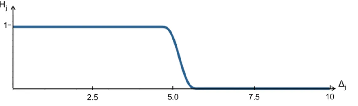
We then use∆j and two hand tuned thresholds∆dand∆s(0 < ∆d < ∆s), to design the tentacle 13 risk function: 14 Hj=        0 if∆j≥∆s 1 2 h 1 + tanh 1 ∆j−∆d + 1 ∆j−∆s i if ∆d<∆j<∆s 1 if∆j≤∆d. (17)

Note thatHj smoothly varies from0, when the dangerous cells associated to tentaclej(if any) are far, to1, 15

when they are near. IfHj = 0, the tentacle is tagged asclear. In practice, threshold∆s must be set to the 16

risk distance for which the context ceases to be safe (H becomes greater than0), so that the robot starts to

17

leave the taught – occupied – path. On the other hand,∆dmust be tuned as the risk distance for which the 18

context becomes unsafe (H = 1), so that the robot follows the best tentacle to circumnavigate the obstacle.

19

In our work, we used the values∆s = 6m and∆d= 4.5m. The risk functionHj corresponding to these 20

values is plotted in Fig. 3.

21

TheHjs of all tentacles are then compared, in order to determineHin (13). Initially, we calculate the 22

path curvatureκ = ω/v ∈ IR that the robot would follow if there were no obstacles. Replacing H = 0 1 in (13), it is: 2 κ=hλx xd−x−jvvs+λϕjϕ˙ϕ i /jωvs,

which is always well-defined, sincejω6= 0and we have setvs>0. We obviously constrainκto the interval 3

of feasible curvatures[−κM, κM]. Then, we derive the two neighbours ofκamong all the existing tentacle 4

curvatures:

5

κn, κnn ∈ Ksuch thatκ∈[κn, κnn).

Let κn be the nearest one, i.e., the curvature of the tentacle that best approximates the safe path2. We 6

2

Without loss of generality, we consider that intervals are defined even when the first endpoint is greater than the second, e.g., [κn, κnn)should be read(κnn, κn]ifκn> κnn.

1 H_j

Δ_j

5.0

2.5 7.5 10

Figure 3: RiskHj, in function of the tentacle risk distance∆j (m) when∆s= 6m and∆d= 4.5m.

denote it as thevisual task tentacle. The situation risk functionHvof that tentacle is then obtained by linear 7

interpolation of its neighbours:

8

Hv =

(Hnn−Hn)κ+Hnκnn−Hnnκn

κnn−κn

. (18)

In practice,Hvmeasures the risk on the visual path, by considering only obstacles on the visual task tentacle 9

and on its neighbour tentacle. In particular, for the context to be safe (i.e., in order to follow the taught path

10

and realize the desired safe task in (6)), it is sufficient that the neighbour tentacles are clear (Hn=Hnn = 0). 11

This way, obstacles on the sides do not deviate the robot away from the taught path.

12

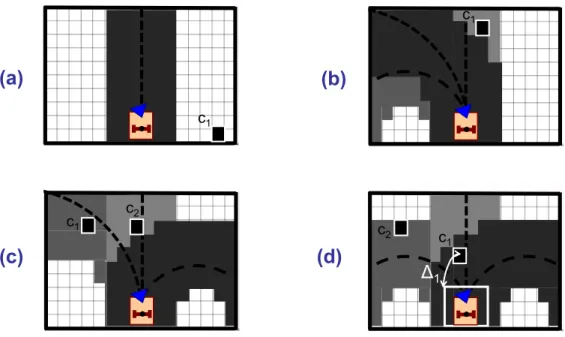
Let us now detail our strategy for determining the best tentacle curvatureκbfor navigation. This strategy 13

is illustrated by the four examples in Fig. 4, where5tentacles are used. In the figure, the dangerous cells

14

(i.e., for each tentaclej, the cells inDjSEj) associated to the visual task tentacle and to the best tentacle 15

are respectively shown in light and dark gray. The occupied cells are shown in black. The best tentacle

16

is derived from the tentacle risk functions defined just above. IfHv = 0(as in Fig. 4(a)), the visual task 17

tentacle can be followed: we setκb = κn, and we apply (13) withH = 0. Instead, if Hv 6= 0, we seek a 18

clear tentacle (Hj = 0). First, to avoid abrupt control changes, we only search among the tentacles between 19

the visual task one and the best one at the previous iteration3, notedκpb, and mid-gray in the figure. If many 20

clear ones are present, the nearest to the visual task tentacle is chosen, as in Fig. 4(b). If none of the tentacles

1

with curvature in[κn, κpb]is clear, we search among the others. Again, the best tentacle will be the clear 2

one that is closest toκnand, in case of ambiguity, the one closest toκnn. If a clear tentacle has been found 3

(as in Fig. 4(c)), we select it and setH = 0. Instead, if no tentacle in K is clear, the one with minimum

4

Hj calculated using (17) is chosen, andH is set equal to thatHj. In the example of Fig. 4(d), tentacle1 5

is chosen and we setH = H1, since∆1 = sup{∆1, . . . ,∆5}, henceH1 = inf{H1, . . . , H5}. Eventual

6

3

IJRR

(d)

Δ

(a)

(b)

(c)

Figure 4: Strategy for selecting the best tentacle among 5 in four different scenarios. The cells associated to the visual task tentacle, to the previous best tentacle, and to the best tentacle are shown in increasingly dark gray; the corresponding tentacles are dashed, and the occupied cellsc1andc2 are shown in black. (a) Since it is clear, the visual task tentacle with curvatureκnis selected:κb =κn. (b) The clear tentacle with

curvature in[κn, κpb]nearest toκnis chosen. (c) Since all tentacles with curvature in[κn, κpb]are occupied,

the clear one nearest to the visual task tentacle is chosen. (d) Since all tentacles are occupied, we select the one with smallestHj, hence, largest risk distance∆j(here,∆1)

given the middle boundary box). ambiguities are again solved first with the distance fromκn, then fromκnn. 7

3.4 Translational Velocity in the Safe Context

8

We will hereby define the translational velocity in the safe contextvs. When the feature motion in the image 9

is fast, the visual tracker is less effective, and the translational velocity should be reduced. This is typically

10

the case at sharp robot turns, and when the camera pan angle ϕis strong (since the robot is far from the

1

taught 3D path). Hence, we definevsas: 2

vs(ω, ϕ) =vm+

vM −vm

4 σ (19)

with functionσdefined as:

3 σ:IR× −π 2, π 2 →[0,4] (ω, ϕ)7→[1+tanh (π−kω|ω|)] [1+tanh (π−kϕ|ϕ|)].

Function (19) has an upper boundvM > 0(forϕ = ω = 0), and smoothly decreases to the lower bound 4

vm > 0, as either|ϕ|or|ω|grow. BothvM andvm are hand-tuned variables, and the decreasing trend is 5

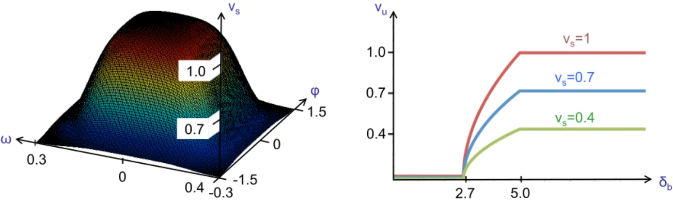
-π/2-π/2 -π/2 -π/2-π/2 -π/2 -0.3 0 0.3 ω φ v_s 0.7 1.0 -1.5 1.5 0 v_u 1.0 δ_b 5.0 2.7 0.4 0.7 0.4 v_s=1 v_s=0.7 v_s=0.4

Figure 5: Left: safe translational velocityvs (ms−1) in function ofω (rads−1) andϕ(rad). Right: unsafe

translational velocityvu (ms−1) in function ofδb(m) for three different values ofvs.

determined by empirically tuned positive parameterskω andkϕ. This definition ofvs yields better results, 6

both in terms of performances and smoothness than the one in [Cherubini and Chaumette 2011], which was

7

only characterized by the imagexvariation. On the left of Fig. 5, we have plottedvsfor:vm = 0.4ms−1, 8

vM = 1ms−1,kω = 13,kϕ = 3. 9

3.5 Translational Velocity in the Unsafe Context

10

The unsafe translational velocity vu must adapt to the potential danger; it is derived from the obstacles 11

on the best tentacle, defined in Section 3.3. In fact, vu is derived from the collision distance δb, which 12

is a conservative approximation of the maximum distance that the robot can travel along the best tentacle

13

without colliding. Since the thinner box contains the robot, ifRfollows the best tentacle, collisions can only

14

occur in occupied cells inC_b. In fact, the collision with cellciwill occur at the distance, denotedδib ≥ 0, 1

that the thinner box would cover along the best tentacle, before touching the center ofci. The derivation of 2

δibis illustrated in Fig. 2 for four occupied cells. 3

Then, we defineδbas the minimum among the collision distances of all occupied cells inCb: 4

δb = inf

ci∈O∩Cb δib.

If all cells inC_b are free, δb = ∞. In the example of Fig. 2, assuming the best tentacle is the straight one 5

(b= 2),δb =δ12. Again, oversizing the box leads to more conservativeδb. 6

The translational velocity must be designed accordingly. Let δdandδs be two hand tuned thresholds 7

such that0 < δd < δs. If the probable collision is far enough (δb ≥δs), the translational velocity can be 8

maintained at the safe value defined in (19). Instead, if the dangerous occupied cell is near (δb ≤ δd), the 9

robot should stop. To comply with the boundary conditionsvu(δd) = 0andvu(δs) =vs, in the intermediate 10

situations we apply a constant deceleration:

11

a=v_s2/2(δd−δs)<0.

Since the distance required for braking at velocityvu(δb)is: 12

δb−δd=−vu2/2a,

the general expression of the unsafe translational velocity becomes:

13 vu(δb) =    vs ifδb ≥δs vs p δb−δd/δs−δd ifδd< δb < δs 0 ifδb ≤δd, (20)

in order to decelerate as the collision distanceδb decreases. In practice, thresholdδdwill be chosen as the 14

distance to collision at which the robot should stop. Instead, thresholdδs must be defined according to the 15

maximum applicable deceleration (notedaM <0), in order to brake before reaching distanceδd, even when 16

the safe velocityvsis at its maximumvM: 17

δs> δd−

2aM

v2_M .

In our work, we usedδd = 2.7m andδs= 5m, as shown on the right of Fig. 5, where we have plottedvu 18

in function ofδb for three values ofvs: 0.4, 0.7, and 1 ms−1. 1

4

Discussion

In this section, we will instantiate and comment our control scheme for visual navigation with obstacle

3

avoidance. Using all the variables defined above, we can explicitly write our controller (13) for visual

4

navigation with obstacle avoidance:

5        v= (1−H)vs+Hvu ω= (1−H)λx(x d_−x)−j vvs+λϕjϕ˙ϕ jω +Hκbvu ˙ ϕ=Hλx(x d_−x)−(j v+jωκb)vu jϕ˙ −(1−H)λϕϕ . (21)

This control law has the following interesting properties.

6

1. In thesafecontext (H= 0), (21) becomes:

7      v=vs ω= λx(x d_−x)−j vvs+λϕjϕ˙ϕ jω ˙ ϕ=−λϕϕ . (22)

In Sect. 3.1, we proved that this controller guarantees global asymptotic stability of the safe task

8

˙

s∗_s. As in [Cherubini et al. 2009] and [Diosi et al. 2011], where obstacles were not considered, the

9

image error is controlled only byω, which also compensates the centroid displacements due tovand

10

toϕ˙ through the image jacobian components (15), to fulfill the visual task (3). The two remaining

11

specifications in (5), instead, are achieved by inputsvandϕ˙: the translational velocity is regulated

12

to improve tracking according to (19), while the camera is driven forward, to ϕ = 0. Note that,

13

to obtain H = 0 with the tentacle approach, it is sufficient that the neighbour tentacles are clear

14

(Hn = Hnn = 0), whereas in the potential field approach used in [Cherubini and Chaumette 2011], 15

even a single occupied cell would generateH >0. Thus, one advantage of the new approach is that

16

only obstacles on the visual path are taken into account.

17

2. In theunsafecontext (H= 1), (21) becomes:

18      v=vu ω=κbvu ˙ ϕ= λx(x d_−x)−(j v+jωκb)vu jϕ˙ . (23)

In Sect. 3.1, we proved that this controller guarantees global asymptotic stability of the unsafe task

19

˙

s∗_u. In this case, the visual task (3) is executed byϕ˙, while the two other specifications are ensured by

20

the2other degrees of freedom: the translational velocity is reduced (and even zeroed tov=vu = 0 21

for very near obstacles such thatδb ≤δd), while the angular velocity makes the robot follow the best 22

tentacle (ω/v = κb). Note that, since no 3D positioning sensor (e.g., gps) is used, closing the loop 23

on the best tentacle is not possible; however, even if the robot slips (e.g., due to a flat tire), at the

24

following iterations tentacles with stronger curvature will be selected to drive it towards the desired

25

path, and so on. Finally, the camera velocityϕ˙ in (23) compensates the robot rotation, to keep the

1

features in view.

2

3. In intermediatesituations (0 < H < 1), the robot navigates between the taught path, and the best

3

path considering obstacles. The situation risk functionHrepresenting the danger on the taught path,

4

drives the transition, but not the speed. In fact, note that, for allH ∈ [0,1], whenδb ≥ δs: v =vs. 5

Hence, a high velocity can be applied if the path is clear up toδs(e.g., when navigating behind another 6

vehicle).

7

4. Control law (21) guarantees that obstacle avoidance has no effect on the visual task, which can be

8

achieved for anyH ∈ [0,1]. Note that plugging the expressions ofv, ω, and ϕ˙ from (21) into the

visual task equation:

10

˙

x=jvv+jωω+jϕ˙ϕ˙ (24)

yields (3). Therefore, desired state xd is globally asymptotically stable for the closed loop

sys-11

tem,∀ H ∈ [ 0, 1]. This is true even in the special case where v = 0. In fact, the robot stops

12

andvbecomes null, if and only ifH= 1andvu = 0, implying thatω = 0andϕ˙ =

λx(xd−x)

jϕ˙ , which

13

allows realization of the visual task. In summary, from a theoretical control viewpoint (i.e., without

14

considering image processing nor field of view or joint limits constraints), this proves that if at least

15

one point inIdis visible, the visual task of driving the centroid abscissa toxdwill be achieved, even

16

in the presence of unavoidable obstacles. This strategy is very useful for recovery: since the camera

17

stays focused on the visual features, as soon as the path returns free, the robot can follow it again.

18

5. Controller (21) does not present local minima, i.e., non-desired state configurations for which u is

19

null. In fact, whenH < 1, u = 0 requires bothvu andvs to be null, but this is impossible since 20

from (19)),vs> vm >0. Instead, whenH = 1, it is clear from (23) that foruto be null it is suffcient 21

thatxd−x= 0andvu = 0. This corresponds to null desired dynamics: s˙∗u = 0(see (9)). This task 22

is satisfied, since pluggingu= 0into (10), yields preciselys˙u = 0 = ˙s∗u. 23

6. If we tune the depth Zcto infinity in (15),jv = 0, andjϕ˙ = jω = 1 +x2. Thus, control law (21) 24 becomes: 25      v= (1−H)vs+Hvu ω= (1−H)λxx d_−x jω + (1−H)λϕϕ+Hκbvu ˙ ϕ=Hλxx d_−x jω −(1−H)λϕϕ+Hκbvu .

Note that, for small image error (x≈xd),ϕ˙ ≈ −ω. In practice, the robot rotation is compensated by

1

the camera pan rotation, which is an expected behavior.

2

5

Simulations

In this section and in the following, we will detail the simulated and real experiments that were used to

4

validate our approach. Simulations are in the video shown in Extension#1.

5

For simulations, we made use of Webots4, where we designed a car-like robot equipped with an actuated

6

320×240pixels70◦ field of view camera, and with a110◦ scanner of range15 m. Both sensors operate

7

at30 Hz. The visual features, represented by spheres, are distributed randomly in the environment, with

8

4

A B C D E F

Tentacles

Figure 6: Six obstacle scenarios for replaying two taught paths (black) with the robot (rectangle): a straight segment (scenarios A to C), and a closed loop followed in the clockwise sense (D to F). Visual features are represented by the spheres, the occupancy grid by the rectangular area, and the replayed paths are drawn in gray.

depths with respect to the robot varying from0.1to100m. The offset betweenR andCisXC = 0.7m,

9

and we setZc = 15m that meets the conditionZc > X

C

2 . We use21tentacles, withκM = 0.35m

−1 _(the

10

robot maximum applicable curvature). For the situation risk function, we use∆s = 6m and∆d = 4.5m. 11

These parameters correspond to the design ofHshown in Fig. 3. The safe translational velocity is designed

12

withvm = 0.4ms−1,vM = 1ms−1,κω = 13andκϕ = 3, as in the graph on the left of Fig. 5. For the 13

unsafe translational velocity, we useδs = 5m, andδd = 2.7m as on the right of Fig. 5 (top curve). The 14

simulations were helpful for tuning the control gains, in all experiments, to:λx = 1andλϕ= 0.5. 15

At first, no obstacle is present in the environment, and the robot is driven along a taught path. Then, up to

16

5obstacles are located, near and on the taught path, and the robot must replay the visual path, while avoiding

17

them. In addition, the obstacles may partially occlude the features. Although the sensors are noise-free, and

1

feature matching is ideal, these simulations allow validation of controller (21).

2

By displacing the obstacles, we have designed the6scenarios shown in Fig. 6. For scenarios A, B and C,

3

the robot has been previously driven along a30m straight path, andN = 8key images have been acquired,

4

whereas in scenarios D, E and F, the taught path is a closed loop of length75m andN = 20key images,

5

which is followed in the clockwise sense. In all scenarios, the robot is able to navigate without colliding,

6

and this is done with the same parameters. The metrics used to assess the experiments are the image error

7

with respect to the visual databasex−xd(in pixels), averaged over the whole experiment and denotede¯,

and the distance, at the end of the experiment, from the final 3D key pose (, in cm). The first metric¯eis

9

useful to assess the controller accuracy in realizing the visual path following task. The latter metric is less

10

relevant, since task (3) is defined in the image space, and not in the pose space.

11

In all six scenarios, path following has been achieved, and in some cases, navigation was completed

12

using only 3image points. Obviously, this is possible in simulations, since feature detection is ideal: in

13

the real case, which includes noise, 3 points may be insufficient. Some portions of the replayed paths,

14

corresponding to the obstacle locations, are far from the taught ones. However, these deviations would

15

have been indispensable to avoid collisions, even with a pose-based control scheme. Let us detail the robot

16

behaviour in the six scenarios:

17

• Scenario A: two walls, which were not present during teaching, are parallel to the path, and three

18

boxes are placed in between. The first box is detected, and overtaken on the left. Then, the vehicle

19

passes between the second box and the left wall, and then overtakes the third box on the right. Finally,

20

the robot converges back to the path, and completes it. Although the walls occlude features on the

21

sides, the experiment is successful, withe¯= 5, and= 23.

22

• Scenario B: it is similar to A, except that there are no boxes, and that the left wall is shifted towards

23

the right one, making the passage narrower towards the end. This makes the robot deviate in order to

24

pass in the center of the passage. We obtain¯e= 6,= 18.

25

• Scenario C: this scenario is designed to test the controller in the presence of unavoidable

obsta-26

cles. Two walls forming a corner, are located on the path. This soon makes all tentacles unsafe:

27

∆j ≤ ∆d| ∀j, yieldingH = 1. Besides, as the robot approaches the wall, the collision distance 28

on the best tentacleδb decreases, and eventually becomes smaller thanδd, to makevu = 0and stop 29

the robot (see (23)). Although the path is not completed (making metricirrelevant), the collision

1

is avoided, and ¯e = 4 pixels. As proved in Section 4, convergence of the visual task (x = xd) is

2

achieved, in spite ofu = 0. In particular, here, the centroid abscissa on the third key image in the

3

database is reached.

4

• Scenario D: high walls are present on both sides of the path; this leads to important occlusions (less

5

than50%of the database features are visible), and to a consequent drift from the taught path.

Never-6

theless, the final key image is reached, without collisions, and withe¯= 34, and= 142. Although

7

this metric is higher than in the previous scenarios (since the path is longer and there are numerous

occlusions), it is still reasonably low.

9

• Scenario E: two obstacles are located on the path, and two other are near the path. The first obstacle

10

is overtaken on the left, before avoiding the second one, also on the left. Then, the robot converges

1

to the path and avoids the third obstacle on the right, before reaching the final key image. We obtain

2

¯

e = 33, and = 74. The experiment shows one of the advantages of our tentacle-based approach:

3

lateral data in the grid is ignored (considering the fourth obstacle, would have made the robot curve

4

away from the path).

5

• Scenario F: here, the controller is assessed in a situation where classical obstacle avoidance strategies

6

(e.g. potential fields) often fail because of local minima. In fact, when detected, the first obstacle is

7

centred on theX axis and orthogonal to it. This may induces an ambiguity, since occupancies are

8

symmetric with respect toX. However, the visual features distribution, and consequent visual task

9

tentacleκndrive the robot to the right of the obstacle, which is thus avoided. We have repeated this 10

experiment with10randomly generated visual feature distributions, and in all cases the robot avoided

11

the obstacle. The scenario involves four more obstacles, two of which are circumnavigated externally,

12

and two on the inside. Here,e¯= 29, and= 75.

13

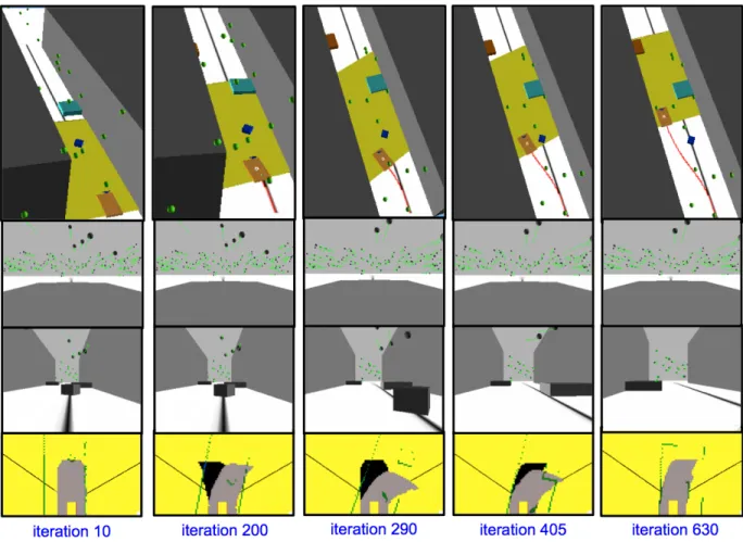
In Fig. 7, we show 5 stages of scenario A. In this figure, as well as later in Fig. 12, in Fig. 14, the

14

segments linking the current and next key image points are drawn in the current image. In the occupancy

15

grid, the dangerous cell sets associated to the visual task tentacle and to the best tentacle (when different)

16

are respectively shown in gray and black, and two black segments indicate the scanner amplitude. Only cells

17

that can activateH (i.e., cells at distance∆< ∆s) have been drawn. At the beginning of the experiment 18

(iteration 10), the visual features are driving the robot towards the first obstacle. When it is near enough, the

19

obstacle triggersH(iteration 200), forcing the robot away from the path towards the best tentacle, while the

20

camera rotates clockwise to maintain feature visibility (iterations 200, 290 and 405). Finally (iteration 630),

21

the controller drives the robot back to the path, and the camera to the forward-looking direction.

22

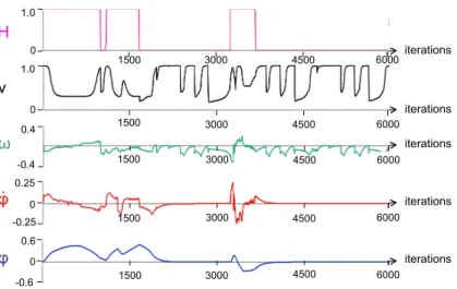
Further details can be obtained by studying some relevant variables. We focus on scenario E, for which

23

we have plotted in Fig. 8 the values ofH,v,ω,ϕ˙, andϕduring navigation. The curve ofHshows when the

24

obstacles, respectively the first (at iterations 0 – 1000), second (1100 – 1700) and third (3200 – 3700), have

25

intervened in control law (21). As aforementioned, the fourth obstacle does not triggerH, since it is too far

26

on the side to jeopardize the robot. Let us now discuss the trend of the five curves. Since the beginning, the

Figure 7: Scenario A. For each of the 5 relevant iterations we show (top to bottom): the robot overtaking the first obstacle, the next key image, the current image, and the occupancy grid.

first obstacle is detected: the tentacle selection induces a negative rotation on the robot (ωcurve), a positive

28

one on the camera (ϕ˙), and a reduction of v. The strategy proves efficient, since the robot overtakes the

29

obstacle. Soon afterwards, the second obstacle triggersH, and provokes a deceleration onv. Concurrently,

30

the camera pan angleϕbecomes positive to track the visual features which are mostly on the left of the

1

robot (just like the taught path, as shown in Fig. 6). When the second obstacle is bypassed, the camera pan

2

is reset to zero. The reduction ofvat iteration 2800 is due only to the sharp turn (i.e., to the reduction ofvs), 3

since the path is safe at this point. Then, the third obstacle triggersH, and is easily circumnavigated. From

4

iteration 3700 onwards, the situation risk function is cancelled. Correspondingly, the variables are driven

5

by (22). Note also that the camera angleϕis reset to 0 in less than 200 iterations, and remains null until the

6

end of the experiment. The small spikes in the angular velocityω, which appear throughout the experiment,

7

correspond to the changes of database key images (except when they are provoked by the obstacles, as

Scenario E webots ijrr- tentacles 0 -0.4 -0.25 1.0 0 0.6 0.25 6000 6000 0 1.0 6000 6000 0 6000 3000 3000 3000 1500 4500 4500 4500 4500 3000 4500 3000 0.4 -0.6 1500 1500 1500 1500 φ φ . ω v H iterations iterations iterations iterations iterations

Figure 8: Evolution of relevant variables in scenario E; top to bottom:H,v(in m s−1),ω(in rad s−1),ϕ˙(in rad s−1), andϕ(in rad).

discussed above).

9

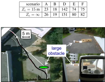
The six simulations have been repeated by setting the feature depthZcto infinity. For all six scenarios, 10

the image accuracy, assessed with e¯, is very near to the one obtained when Zc = 15 m. On the other 11

hand, the pose accuracy, assessed with, is lower when Zc = ∞, as shown in Table 1. The difference 12

is relevant on long paths (scenarios D, E and F). Although the navigation task is defined in the image

13

space, these experiments show that tuningZc, even coarsely, according to the environment, can contribute 14

to the controller performance in the 3D space. This aspect had already emerged in part in our previous

15

work [Cherubini et al. 2009].

16

6

Real Experiments

After the simulations, the framework has been ported on our CyCab vehicle, set in car-like mode (i.e.,

18

using the front wheels for steering), for real outdoor experimental validation. The robot is equipped with

1

a coarsely calibrated 320×240 pixels 70◦ field of view, B&W Marlin (F-131B) camera mounted on a

2

TRACLabs Biclops Pan/Tilt head (the tilt angle is null, to keep the optical axis parallel to the ground), and

3

with a 2-layer, 110◦ scanning angle, laser SICK LD-MRS. A dedicated encoder on the TRACLabs head

4

precisely measures the pan angleϕrequired in our control law (see (21)). The grid is built by projecting

5

the laser readings from the 2 layers on the ground. Exactly the same configuration (i.e., same parameters,

6

gains and grid size) tuned in Webots is used on the real robot. The centroid depth value that we used in

7

simulations (Zc= 15m) proved effective in all real experiments as well, although the scenarios were very 8

Table 1: Final 3D error (in cm) when Zc = 15m and Zc = ∞ (for scenario C, since the path is not completed,is irrelevant). scenario A B D E F Zc= 15m 23 18 142 74 75 Zc=∞ 26 19 151 80 82 journal paper large obstacle 5 m

Figure 9: Scenario A (a long obstacle is avoided): taught (white) and replayed (black) paths. variegate. This confirms, as shown in [Cherubini et al. 2009], that a very coarse approximation of the scene

9

depth is sufficient to effectively tuneZc. The velocity (vM = 1, as in Webots) has been reduced due to the 10

image processing rate (10 Hz), to limit the motion of features between successive images; the maximum

11

speed attainable by the CyCab is1.3ms−1 anyway. Since camera (10Hz) and laser (12.5Hz) processing

1

are not synchronized, they are implemented on two different threads, and the control inputuderived from

2

control law (21) is sent to the robot as soon as the visual information is available (10Hz).

3

It is noteworthy to point out that the number of tentacles that must be processed, and correspondingly,

4

the computational cost of the laser processing thread, increase with the context danger. For clarity, let us

5

discuss two extreme cases: a safe and an occupied contexts. To verify that a context is safe (i.e., thatHv = 0 6

in (17)), all the cells in the dangerous areasDS

E of only the two neighbour tentacles must be explored.

7

Instead, in a scenario where the grid is very occupied, all of the tentacles inKmay need to be explored. In

8

general, this second case will be more costly than the first. However, in practice, since only the minimum

9

risk and collision distances (∆j and δb) are required by our controller, exploration of a tentacle stops as 10

soon as the nearest cell is found occupied, so that the tentacles are rarely entirely explored. The experiments

11

showed that the computational cost of laser processing, using the chosen number of tentacles (i.e., 21, as

12

mentioned in Sect. 2.3), was never a critical issue with respect to that of image processing.

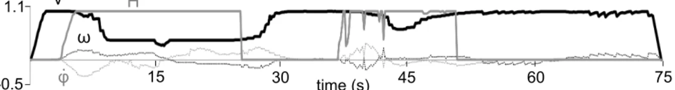
First, we have assessed the performance of our control scheme when a very long obstacle is positioned

14

perpendicularly on the taught path (denoted path A, and shown in Fig. 9). In Fig. 10, we have plotted the

15

control inputsu, and the situation risk functionH. The smooth trend ofuat the beginning and end of the

16

experiments is due to the acceleration saturation carried out at the CyCab low-level control. The obstacle

17

is overtaken on the left, while the camera rotates right to maintain scene visibility (dotted black and dotted

18

gray curves in Fig. 10). The robot is able to successfully reach the final key image and complete navigation,

19

although it is driven over5meters away from the taught 3D path by the obstacle. In practice, soon after the

20

obstacle is detected (i.e., after5 s), tentacles with first positive (5−16s), and then negative (16−25s)

21

curvature are selected. Since these tentacles are clear,vis reduced only for visual tracking, by (19) (solid

22

black curve in Fig. 10). This is a major feature of the tentacle method, which considers only the actual

23

collision risk of obstacles for reducing the translational velocity. After25s, the environment returns clear

1

(H = 0), so the visual tentacle can be followed again, and the robot is driven back to the path. Then

2

(38−52s) a small bush on the left triggersH and causes a small counterclockwise rotation along with a

3

slight decrease inv. Then the context returns safe, and the visual path can be followed for the rest of the

4

experiment. The translational velocity averaged over the experiment is0.79ms−1, which is more than twice

5

the speed reached in [Cherubini and Chaumette 2011].

6

After these results, we have run a series of experiments, on longer and more crowded paths (denoted

7

B to E on Fig. 11) on our campus. All campus experiments here are also visible in the video shown in

8

Extension #2. The Cycab was able to complete all paths (including 650m long path E), while dealing

9

with various natural and unpredictable obstacles, such as parked and driving cars and pedestrians. The

1

translational velocity averaged over these experiment was0.85ms−1.

2

Again, by assessing the collision risk only along the visual path, non-dangerous obstacles (e.g., walls or

3

cars parked on the sides) are not taken into account. This aspect is clear from Fig. 12(left), where a stage

4

of the navigation experiment on path E is illustrated. From top to bottom, we show: the next key image

5

in the databaseId, the current imageI, and three consecutive occupancy grids processed at that point of 6

IJRR-pathA long obstacles tent 1.1 -0.5 φ 15 30 time (s) 45 60 75 . ω v H

Figure 10: Control inputs in scenario A:v(solid black, in ms−1),ω (dotted black, rads−1) ϕ˙ (dotted gray, rads−1) andH (solid gray).

Figure 11: Map of the four navigation paths B, C, D, E.

the experiment. As the snapshots illustrate, the cars parked on the right (which were not present during

7

teaching) do not belong to any of the visual task tentacle classification areas. Hence, they are considered

8

irrelevant, and do not deviate the robot from the path.

9

Another nice behaviour is shown in Fig. 12(center): if a stationing car is unavoidable, the robot

deceler-10

ates and stops with (20), but, as soon as the car departs, the robot gradually accelerates (again with (20)), to

11

resume navigation. In fact, as we mentioned in Section 4, when the best tentacle is clear up to distanceδs, a 12

high velocity can be applied: v =vs, independently from the value ofH. In the future, this feature of our 13

approach could even be utilized for vehicle following.

14

An experiment with a crossing pedestrian is presented in Fig. 12(right). The pedestrian is considered

15

irrelevant, until it enters the visual task tentacle (second image). Then, the clockwise tentacles are selected

16

to pass between the person and the right side walk. When the path is clear again, the robot returns to the

17

visual task tentacle, which is first counter-clockwise (fourth image) and then straight (fifth image).

18

In October 2011, as part of the final demonstration of the French ANR project CityVIP, we have validated

19

our framework in a urban context, in the city of Clermont Ferrand. The experiments have taken place in the

20

crowded neighbourhood of the central square Place de Jaude, shown in Fig. 13. For four entire days, our

21

Cycab has navigated autonomously, continuously replaying a set of visual paths of up to700m each, amidst

22

a variety of unpredictable obstacles, such as cars, pedestrians, bicycles and scooters. In Fig. 14, we show

1

some significant snapshots of the experiments that were carried out in Clermont Ferrand. These include

2

photos of the Cycab, as well as images acquired by the on-board camera during autonomous navigation.

3

These experiments are also visible in the video shown in Extension#3.

4

In Fig. 14(a-c), Cycab is moving in a busy street, crowded with pedestrians and vehicles. First, in

5

Fig. 14(a), we show a typical behaviour adopted for avoiding a crossing pedestrian: here, Cycab brakes as

6

a lady with black skirt crosses the street. The robot would either stop or circumnavigate the person, and in

Figure 12: Validation with: irrelevant obstacles (left), traffic (center) and a moving pedestrian (right). The visual task tentacle and best tentacle (when different) are respectively indicated as VTT and BT in the occupancy grids.

four days no one has ever even closely been endangered nor touched by the vehicle. In many experiments,

8

Cycab has navigated among fast moving vehicles (cars in Fig. 14(b), and a scooter in 14(c)), and manual

9

security intervention was never necessary. The robot has also successfully avoided many fixed obstacles,

10

including a stationing police patrol (Fig. 14(d)) and another electric vehicle (Fig. 14(e)). Obviously, when

1

all visual features are occluded by an obstacle or lost, the robot stops.

2

Moreover, we have thoroughly tested the behaviour of our system with respect to varying light, which

3

is an important aspect in outdoor appearance-based navigation. Varying light has been very common in the

4

extensive Clermont Ferrand experiments, which would last the whole day, from the first light to sunset, both

5

with cloudy and clear sky. In some experiments, we could control the robot in different lighting conditions,

Figure 13: City center of Clermont Ferrand, with one of the navigation paths where the urban experiments have been carried out.

using the same taught database. For instance, Fig. 14(f) shows two images acquired approximately at the

7

same position at5p.m. (top) and11a.m. (bottom), while navigating with the same key images. However, in

8

spite of the robustness of the image processing algorithms. which has been proved in [Royer et al. 2007], in

9

some cases (e.g., when the camera was overexposed to sunlight), the visual features required for navigation

10

could not be detected. Future work in adapting the camera automatic shutter settings should solve this issue.

11

In the current version of our framework, moving obstacles are not specifically recognized and modelled.

12

Although, as the experiments show, we are capable of avoiding slowly moving obstacles (e.g., crossing

13

pedestrians or baby pushchairs as in Fig. 14(g)), the main objective of our future work will be to directly

14

tackle this problem within the control law, in order to avoid fast obstacles as well. This can be done, for

15

example, by estimating the velocity of the detected objects, and then using it to predict their future position.

16

In our opinion, the main difficulty, in comparison with the case of static obstacles, will concern the accuracy

17

and computation cost of this estimation process.

18

Overall, Cycab has navigated using an average of approximately sixty visual points on each image, and

19

some paths have even been completed using less than30points. Along with all the cited technical aspects,

20

the experiments highlighted the reactions of non-robotic persons to the use of autonomous ground vehicles

21

in everyday life. Most passer-bys had not been informed of the experiments, and responded with curiosity,

22

surprise, enthusiasm, and - rarely - slight apprehension.

23

7

Conclusions

A framework with simultaneous obstacle avoidance and outdoor vision-based navigation, without any 3D

25

model or path planning has been presented. It merges a novel, reactive, tentacle-based technique with

26

visual servoing, to guarantee path following, obstacle bypassing, and collision avoidance by deceleration.