Computer Engineering and Applications Vol. 7, No. 2, June 2018
A Distance-Reduction Trajectory Tracking Control Algorithm
for a Rear-Steered AGV
Anugrah K. Pamosoaji
Faculty of Industrial Technology, Universitas Atma Jaya Yogyakarta, Indonesia School of Mechanical Engineering, Pusan National University, Busan, South Korea
ABSTRACT
This paper presents a Lyapunov-based switched trajectory tracking control design for a rear-steered automated guided AGV (AGV). Given a moving reference whose position and orientation have to be tracked by the AGV, the main objective of the controller is to reduce AGV’s distance from the reference while adjusting its orientation. The distance reduction issue is important, especially in huge warehouses operating a group of AGVs, since the rate of AGV-to-reference distance reduction contributes to the possibility of AGV-to-AGV collision. A set of control algorithms is proposed to handle large AGV’s orientation. Simulations that show the performance of the proposed method is presented.
Keywords: Tracking Control, Automated Guided AGV, Distance Reduction, Collision Avoidance.
1. INTRODUCTION
Trajectory tracking for AGVs has been studied for decades. This issue becomes important when an AGV groups start to operate in a large workspace, such as warehouse. Here, one of the aspects of a warehouse is order-picking mechanism [1]. In association with the use of AGVs, warehouse management area mostly discusses about mechanism to generate AGV trajectory plan [2-4]. In robotics, the realizations of the plan have been addressed under a typical terminology, i.e., “trajectory tracking”.
A huge number of tracking strategies have been developed. Roughly speaking, developments of tracking algorithm for AGVs can be divided into two directions: first, path tracking which focused on the placement of a physical AGV to a planned path. Research on this issue was established in [5-9]. The second type of this study is trajectory tracking, which is focused on the placement of physical AGV to the reference at any time instance. Several works applied Cartesian coordinate system to express the AGV’s configuration [10-12]. Such the type of methods has a complexity in controlling AGV-to- target distance that is necessary especially for the problem of tracking moving preplanned references in multiple AGV systems.
Inter-AGV collision avoidance has been an interesting issue. Various approaches to this problem have been proposed. They can be categorized according to two paradigms: those involving communication among the AGVs in a group, and those with no such communication. In the first paradigm, the communication among AGVs became an important consideration regarding to performance of decentralized control and coordination [5-10]. In [6], the problem of conflict resolution for multiple AGVs was treated, focusing on the goal reachability and safety guarantee.
In this approach, right-turn-only policy was followed. In [7], decentralized navigation of groups of nonholonomic wheeled mobile robots was proposed. Maintenance of inter-robot distances while the leader moved along collision-avoidance trajectories was focused. In line with [6], the work in [8] proposed an approach named Resource Allocation Systems for free-ranging multi-AGV systems. Bekris et al. investigated the coordination of the motions of second-order robots in consideration of planning-cycle differences [10].
A plan in warehouse management is a good plan if it is trackable in a finite time. The tractability of the plan is indicated by the ability of the controller to reduce the distance between the AGV and the plan. This problem can be solved by, first, using a polar coordinate system, since one of its axis can represent such the distance. Some trajectory tracking controls using polar coordinate system are reported in [12-18]. The works in [17] and [18], for instance, proposed a class of model predictive control for trajectory tracking. In [14], an error-based control for robust trajectory tracking for unmanned ground AGVs.
However, most publications lack of concerning the reducing AGV-to-reference distance under extreme AGV’s orientation. This issue is important, since mostly, at the beginning the initial configuration of the AGV is not the same with the plan. Moreover, it is possible that the AGV starts to track the assigned plan from extreme orientation in polar coordinate system. If the AGV disable to track the plan, under a crowded circumstance, it is possible that a collision between the AGV to another single one is inevitable.
In this paper, a control algorithm is designed to drive a rear-steered AGV to its respective reference focusing on decreasing distance between the AGV and the reference. The contribution of this study is twofold: first, the design of controller to minimize collision to other AGVs with their own plans. Second, the controller answers question of reducing AGV-to-reference distance even the initial navigation angles are extreme. The organization of this paper is as follows. Section 2 describes the problem definition; Section 3 explains the proposed controller design; Section 4 presents the simulation results; and Section 5 concludes this paper.
2. PROBLEMDEFINITION
Suppose that there exists a rear-steered AGV whose location is represented by the coordinate (𝑥, 𝑦) and orientation by 𝛿 as shown in Figure 1. The AGV has to drive its controlled point 𝑃 with traction velocity 𝑢 and angular velocity 𝜔; 𝑙 represents the distance between the centers of actuation 𝑂. The AGV itself has two actuators, i.e., velocity 𝑣 and steering 𝛿. The kinematic model of the AGV is given as,
𝑥 = 𝑣cos𝜃cos𝛿 (1) 𝑦 = 𝑣sin𝜃cos𝛿 (2) 𝜃 = −(𝑣 𝑙 )sin𝛿 (3)
Computer Engineering and Applications Vol. 7, No. 2, June 2018 Actual AGV Reference v
(velocity and orientation) of the reference is predefined and is represented by its traction and angular velocities, i.e., 𝑣𝑟 and 𝜔𝑟, respectively.
For tracking control design purpose, we define navigation variables (𝜌, 𝛼, 𝜑) formulated as
𝜌 = 𝛥𝑥2+ 𝛥𝑦2 (4)
𝛼 = arctan2(𝛥𝑦, 𝛥𝑥) − 𝜃 (5) 𝜑 = 𝜃𝑔 − arctan2(𝛥𝑦, 𝛥𝑥) (6)
where 𝛥𝑥 = 𝑥𝑟 − 𝑥, 𝛥𝑦 = 𝑦𝑟− 𝑦. In this paper, we address a problem of trajectory
tracking control for extreme navigation angles 𝛼 and 𝜑, i.e., at least one of the following conditions occurs:
𝜋 2 < 𝛼 ≤ 𝜋 ∪ −𝜋 < 𝛼 < −𝜋 2 (7) 𝜋 2 < 𝜑 ≤ 𝜋 ∪ −𝜋 < 𝜑 < −𝜋 2 (8)
FIGURE 3. Multiple-AGV trajectory tracking problem near a conflict point
The situation to address is shown in Figure 3. Suppose that two AGVs follow their own plan (reference) and assume that their plans have intersection at point P. Assume that the plan is predefined such that if each AGV occupies the desired trajectory, inter-AGV collision can be avoided. Therefore, a control mechanism must be designed to reach the collision-free motion. However, since the AGVs are nonholonomic, the orientations of the AGVs contribute to the motion. In most cases, initial orientation sometimes prohibits the AGV to decrease the AGV-to-AGV distance.
The extreme initial navigation angles appear in [14-15] for point stabilization problem. In the problem, the control law has no effect of reference’s velocities since its velocities are zero. However, for the case of moving reference, the reference’s motion influences the evolution of navigation variables in Equations (4)-(6). The evolution of the navigation variables is described as follows,
𝑞 (𝑡) = 𝑓 𝑞, 𝑞(0) = 𝑞0 (9) where r r r r r cos sin sin sin cos sin sin cos cos cos v v l v v v v v f (10) 𝑞(𝑡) = 𝜌 𝛼 𝜑 𝑇 (11)
The objective of this paper is twofold. First is to design a trajectory tracking algorithm such that,
lim 𝑡→∞𝜌 ≤ 𝜌ss (12) AGV 1
1
h,1
h,2
2 P AGV 2 AGV 1's reference AGV 2's referenceComputer Engineering and Applications Vol. 7, No. 2, June 2018 lim
𝑡→∞𝛼 ≈ 0, (13)
lim
𝑡→∞𝜑 ≈ 0, (14)
where 𝑡 represents time and 𝜌ss is maximum steady-state distance. Second, the paper
identifies necessary and sufficient conditions such that the distance is kept decrease. The dynamics of the actuator is derived by the following steps. Note that the parameters used in the dynamics are described in Table 1. The torques applied to the driving and steering motors are formulated as,
𝜏dr = 𝐼dr𝜔 dr+ 𝐵dr𝜔dr+ 𝐹dr𝑟dr. (15)
𝜏𝛿 = 𝐼𝛿𝜔 𝛿 + 𝐵𝛿𝜔𝛿 (16)
TABLE 1.
Dynamics symbols and definitions
Symbol Definition
𝜏dr and 𝜏𝛿 Torque produced by the driving and steering motors, respectively.
𝐹dr Traction force applied to the driving motor.
𝐼dr and 𝐼𝛿 Moment of inertia of the driving wheel controlled by the driving and steering motors, respectively.
𝜔drand 𝜔𝛿 angular velocity of the driving and steering motors,
respectively.
𝐵dr and 𝐵𝛿 viscous friction coefficient of the driving and steering motors, respectively.
𝑟dr radius of the driving wheel.
𝑘a, dr and 𝑘a, 𝛿 torque constant of the driving and streering motors, respectively.
𝑘b, dr and 𝑘b, 𝛿 voltage constant of the driving and steering motors,
respectively.
𝑅dr and 𝑅𝛿 electric resistance constants of the driving and steering motors, respectively.
𝑢𝑣 and 𝑢𝛿 input voltage applied to the driving and steering
The model of driving and steering motors are described as
𝜏dr = 𝑘a, dr(𝑢𝑣− 𝑘b, dr𝜔dr) /𝑅dr, (17)
𝜏𝛿 = 𝑘a, 𝛿(𝑢𝛿 − 𝑘b, 𝛿𝜔𝛿) /𝑅𝛿. (18)
Substitute Equation (17) to Equation (15) yields
𝐼dr𝑅dr 𝑘a, dr 𝜔 dr+ 𝐵dr𝑅dr+𝑘a, dr𝑘b, dr 𝑘a, dr 𝜔dr+ 𝐹dr𝑅dr𝑟dr = 𝑘𝑃,𝑣(𝑣 dr− 𝑣dr) − 𝑘𝐷,𝑣𝑣 dr. (19) Since 𝜔dr = 𝑣dr
𝑟dr, then Equation (19) is rewritten as
dr dr a, dr dr dr , D * dr dr , P 2 dr dr dr v k R I r k v r k r R F v v P, dr dr dr a, dr b, dr a, dr dr v r k k k k R B v (20)
where vdr* is the planned driving velocity of the AGV. Since
dr dr dr dr r v I F ,
then Equation (20) is rewritten as
dr dr dr dr dr a, dr , D 1 v R I r k r k v P, dr dr dr a, dr b, dr a, dr dr v r k k k k R B v kP,vrdrvdr* 0 (21) Substitution of (18) to (16) yields a, b, a, a, k k k R B k R I * D, , P ( ) k k (22)
where * is the planned steering angle of the AGV. Time derivative of Equation (22) is as follow,
Computer Engineering and Applications Vol. 7, No. 2, June 2018 D, a, b, a, a, k k k k R B k R I 0 ) ( * , P k (23) 3. CONTROLDESIGN
A control algorithm is designed to accommodate extreme configuration. The proposed control is Lyapunov-based control which is consists of two parts, i.e., distance reduction and orientation controls.
3.1 DISTANCE-REDUCTION CONTROL
The purpose of distance control is to drive the AGV such that Equation (12) is satisfied. For this type of control, we propose switched traction velocity control, as explained in Propositions 2 and 3. The idea is in this control, we regard only one actuator, i.e., 𝑣 and the other one, i.e., steering actuator 𝛿 as a parameter.
Proposition 1: The following properties lead to𝜌 < 0:
1) 𝑣cos𝛼 > 0. (24)
2) 𝑣cos𝛼 < 0 and 𝑣𝑟cos𝜑 < 𝑣cos𝛼. (25)
Proof: Suppose that 𝜌 < 0. The first equation of Equation (10) can be rewritten as
𝑣𝑟cos𝜑 − 𝑣cos𝛼cos𝛿 = 𝑤, (26)
where 𝑤 < 0. (26) can be rewritten as
cos𝛿 =−𝑤+𝑣𝑟cos𝜑
𝑣cos𝛼 . (27)
Since 0 ≤ cos𝛿 ≤ 1, then the value of the right side of (27) must be in the interval of [0, 1]. In other words, 0 ≤ −𝑤 + 𝑣𝑟cos𝜑 𝑣cos𝛼 −1 ≤ 1. Suppose that
𝑣cos𝛼 > 0 and 𝑣𝑟cos𝜑 ≥ 0. Then we have the following admissible range of 𝑤.
𝑣𝑟cos𝜑 ≥ 𝑤 ≥ −𝑣cos𝛼 + 𝑣𝑟cos𝜑 (28)
It is clear that 𝑣𝑟cos𝜑 − 𝑣cos𝛼 < 𝜌 < 0, which confirms that the lower bound of 𝑤 is negative. In addition, since 𝑣𝑟cos𝜑 ≥ 0, the upper bound of 𝑤 is zero to satisfy Equation (26). Therefore, 𝑤 spans in the interval −𝑣cos𝛼 + 𝑣𝑟cos𝜑 ≤ 𝑤 ≤ 0. For
𝑣cos𝛼 > 0 and 𝑣𝑟cos𝜑 ≤ 0, the admissible range of 𝑤 is the same with Equation
(28). Since the upper bound of 𝑤 is negative, then in this condition 𝜌 is always negative.
The next case is when 𝑣cos𝛼 < 0 and 𝑣𝑟cos𝜑 ≥ 0. In this situation, we have the following admissible range of 𝑤.
𝑣𝑟cos𝜑 ≤ 𝑤 ≤ −𝑣cos𝛼 + 𝑣𝑟cos𝜑. (29)
Since the lower and upper bounds of 𝑤 is non-negative, we can conclude that 𝜌 is always positive in this condition. The last condition to check is when 𝑣cos𝛼 < 0 and 𝑣𝑟cos𝜑 < 0. The admissible range of 𝑤 is in the same form with Equation (29). Hence, the upper bound of 𝑤 would be negative if and only if 𝑣𝑟cos𝜑 < 𝑣cos𝛼.
Proposition 2: Suppose that cos𝛿 > 0. Define 𝜓 = cos𝛼cos𝛿. For 𝑣𝑟cos𝜑 < 0, the following traction velocity control.
𝑣 = −𝑘𝑣,1sgn 𝜓 𝑣𝑟cosφψ−1 (30)
where 0 < 𝑘𝑣,1 < 1 is a constant, makes the AGV-to-reference 𝜌 closer to zero.
Proof: Define a Lyapunov candidate function
𝑉1 = 0.5𝑘𝜌𝜌2. (31)
The first time derivative of 𝑉1 is
𝑉 1 = 𝑘𝜌𝜌𝜌 . (32)
Substitution of Equation (11) to Equation (32) yields
𝑉 1 = −𝑘𝜌𝜌𝑣𝜓 + 𝑘𝜌𝜌𝑣𝑟cos𝜑 (33)
The AGV-to-reference 𝜌 tends to zero if 𝑉 1 < 0. Under the condition of 𝑣𝑟cos𝜑 < 0 and 𝜓 < 0, the substitution of Equation (30) to Equation (33) yields 𝑉 1 = − 1 − 𝑘𝑣,1 𝑘𝜌𝜌 𝑣𝑟cos𝜑 ,which can be less than zero if and only if 0 < 𝑘𝑣,1 < 1. The similar analysis for 𝑣𝑟cos𝜑 < 0 and 𝜓 > 0 yields 𝑉 1 = 𝑘𝑣,1 − 1𝑘𝜌𝜌𝑣𝑟cos𝜑, which leads to 𝑉1<0 if 0<𝑘𝑣,1<1.
Proposition 3: Suppose that cos𝛿 > 0. For 𝑣𝑟cos𝜑 > 0, the following traction velocity control
Computer Engineering and Applications Vol. 7, No. 2, June 2018 where
𝑘𝑣,2 > 1 + 𝜓 𝑣 / 𝑣𝑟cos𝜑 −1 (35)
is a constant, makes the AGV-to-reference 𝜌 closer to zero.
Proof: The proof can be made by using the same Lyapunov candidate function in Proposition 2. Under the condition of 𝑣𝑟cos𝜑 > 0 and 𝜓 < 0, the substitution of Equation (34) to Equation (33) yields 𝑉 1 = 𝑘𝜌𝜌 𝑣𝑟cos𝜑 − 𝑘𝑣,2 𝑣𝑟cos𝜑 + 𝜓 𝑣 , which is negative definite if 𝑘𝑣,2 satisfies Equation (35). The same result can be obtained for the other condition, i.e., 𝑣𝑟cos𝜑 > 0 and 𝜓 > 0.
3.2 ORIENTATION CONTROL
The purpose of orientation control is to drive the AGV such that Equations (13)-(14) are satisfied. Here, as explained in Propositions 4 and 5, we regard 𝛿 as the actuator and 𝑣 as a parameter. Define a constant 𝜆 > 0 and a coefficient 𝑘𝑣,3 that describes the relation between 𝑣 and 𝑣𝑟 as follows.
𝑣𝑟sin𝜑 = 𝑘𝑣,3𝑣sin𝛼 (36) In addition, define
otherwise, , 1 ] 2 / , 2 / [ if , 1 cos 2 / 1 2 2 / 1 2 h h (37) otherwise, , ] , 0 [ if , sin h h (38) and ∈ [0, 1].Define another Lyapunov candidate function
𝑉2 = 0.5𝑘𝜌 𝛼2 + 𝜑2 , (39)
where 𝑘𝜌 > 0 is constant. The first time derivative of 𝑉2 is
where
𝑉 21= 𝑣𝑟sin𝜑 − 𝑣sin𝛼cos𝛿 𝜑 − 𝛼 𝜌 (41)
𝑉 22 = (𝛼𝑣 𝑙 )sin𝛿 + φω𝑟 (42)
We can state the following proposition.
Proposition 4: The following steering control
otherwise, , tan , 0 1 / if , tan 1 1 2 1 1 h h (43) where 𝛾1 = 𝑘𝑣,3+ 𝜆12𝜌𝑣sin𝛼 𝜑 − 𝛼 −2 − 1, 𝜆1 > 0, and 𝑘𝑣,3 > 0, drives 𝛼 and 𝜑 to zero, under the necessary condition of
𝑘𝑣,3+ 𝜆12𝜌𝑣sin𝛼 𝜑 − 𝛼
2
≤ 1 (44)
Proof: We have to proof that 𝑉 21≤ 0 for all
𝑉 21 = 𝑣𝑟sin𝜑 − 𝑣sin𝛼cos𝛿 𝜑 − 𝛼 𝜌, 𝛼 ∈ [−𝜋, 𝜋] and 𝜑 ∈ [−𝜋, 𝜋]. Substitution of Equation (37) to Equation (41) yields.
𝑉 21= 𝑣𝑟sin𝜑 − 𝑣sin𝛼 1 − 2 𝜑 − 𝛼 𝜌. (45)
Therefore Equation (45) can be rewritten as
𝑉 21= 𝑘𝑣,3− 1 − 2 1 2 𝑣sin𝛼 𝜑 − 𝛼 𝜌 (46)
Computer Engineering and Applications Vol. 7, No. 2, June 2018 otherwise, , ] , 0 [ if , h (47) where, 𝜙 = 1 − 𝑘𝑣,3 + 𝜆12𝜌𝑣sin𝛼 𝜑 − 𝛼 2 (48)
Substitution of in Equation (47) to Equation (46) yields
𝑉 21= −𝜆12𝑣2sin2𝛼 𝜑 − 𝛼 2< 0. (49)
Equation (49) concludes that 𝑉 21< 0 under the necessary condition Equation (44). The control law in Equation (43) can be obtained from substituting Equation (47) to Equation (37) and Equation (38).
Proposition 5: The following control law
otherwise, , tan , 0 1 if , tan 2 1 2 2 1 h h (50) where 𝛾2 = 𝑘𝑣,3+𝜆12𝜌𝑣sin𝛼 𝜑−𝛼 2 1− 𝑘𝑣,3+𝜆12𝜌𝑣sin𝛼 𝜑−𝛼 2 −1 (51) drives 𝑉 21< 0 and 𝑉 22< 0.
Proof: Let in Equation (38) is defined as
= −𝑙𝜆22𝛼𝑣. (52) Substitution of in Equation (52) to Equation (42) yields
In addition, to make Equation (51) decreases 𝑉21, 𝜆2 must be set such that the
following equation is satisfied;
1 − 𝑘𝑣,3 + 𝜆12𝜌𝑣sin𝛼 𝜑 − 𝛼
2
= −𝑙𝜆22𝛼𝑣. (54)
From Equation (54), we obtain the formulation of 𝜆2 as follows;
𝜆2 = 1 − 𝑘𝑣,3+ 𝜆12𝜌𝑣sin𝛼 𝜑 − 𝛼
2
/𝑙2𝛼2𝑣2
4
. (55)
It is straightforward that substitution of 𝜆2 in Equation (55) to Equation (52)
followed by substitution of Equation (52) to Equation (37) yields Equation (51).
Proposition 6: The necessary condition to guarantee 𝑉 2 < 0 is 𝑘𝑣,3 = 𝑘𝑣,4 1 − 2𝜆12𝜌𝑣sin𝛼 𝜑 − 𝛼 . (56)
where 0 < 𝑘𝑣,4 ≤ 1 is a constant.
Proof: From the control law in Equation (43), it is clear that 𝑘𝑣,3 ≤ 1 − 𝜆12𝜌𝑣sin𝛼 𝜑 − 𝛼 to make the argument of tan−1 real. Also, from the control law
in Equation (51), the range of 𝑘𝑣,3 must be 𝑘𝑣,3 ≥ −𝜆12𝜌𝑣sin𝛼 𝜑 − 𝛼 to guarantee
𝑉 2 < 0. In summary, we can conclude that the range of 𝑘𝑣,3 is
−𝜆12𝜌𝑣sin𝛼 𝜑 − 𝛼 ≤ 𝑘𝑣,3 ≤ 1 − 𝜆12𝜌𝑣sin𝛼 𝜑 − 𝛼 (57)
By letting 𝑘𝑣,3 = 𝑘𝑣,4 1 − 2𝜆12𝜌𝑣sin𝛼 𝜑 − 𝛼 , we can guarantee that 𝑘𝑣,3 satisfies
Equation (42). Therefore, this proposition is proofed. According to Equation (56), the range of 𝑘𝑣,3 can be enlarged by increasing the value of 𝜆1.
4. SIMULATIONRESULTS
For the AGV, 𝑥 = 10 m, 𝑦 = 10 𝑚, 𝜃 = 45°. The reference starts from 𝑥𝑟 = 10 m, 𝑦𝑟 = −10 m, 𝜃 = 90°. Therefore, the initial navigation variables are 𝜌 = 20 𝑚, 𝛼 = −135°, and 𝜑 = 180°. The initial values of the AGV’s actuators are 𝑣 = 0 m/s and 𝛿 = 0 °. The reference’s velocities are 𝑣𝑟 = 2 m/s and 𝜔𝑟 = 10 °/s.
Here, the following parameters are applied: 𝜆1 = 100, 𝑘𝑣,4= 0.1, 𝑘𝑣,4 = 0.5
and 𝑘𝑣,4 = 0.9. The generated path for 𝑘𝑣,4 = 0.1 is shown in Figure4. All simulations show similar pattern in distance reduction. There are three phases of distance reduction under extreme initial orientations, as shown in Figure 5.
Computer Engineering and Applications Vol. 7, No. 2, June 2018
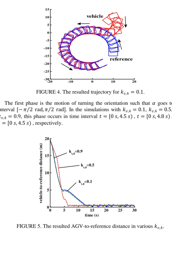
FIGURE 4. The resulted trajectory for 𝑘𝑣,4 = 0.1.
The first phase is the motion of turning the orientation such that 𝛼 goes to the interval [− 𝜋 2 rad, 𝜋 2 rad]. In the simulations with 𝑘𝑣,4 = 0.1, 𝑘𝑣,4 = 0.5, and 𝑘𝑣,4 = 0.9, this phase occurs in time interval 𝑡 = [0 𝑠, 4.5 𝑠) , 𝑡 = [0 𝑠, 4.8 𝑠) , and 𝑡 = [0 𝑠, 4.5 𝑠) , respectively.
FIGURE 5. The resulted AGV-to-reference distance in various 𝑘𝑣,4.
-20 -10 0 10 20 -30 -25 -20 -15 -10 -5 0 5 10 15 reference vehicle 0 5 10 15 20 25 30 0 5 10 15 20 time (s) v e h ic le -t o -r e fe r e n c e d is ta n c e ( m ) k v,4=0.1 k v,4=0.5 k v,4=0.9
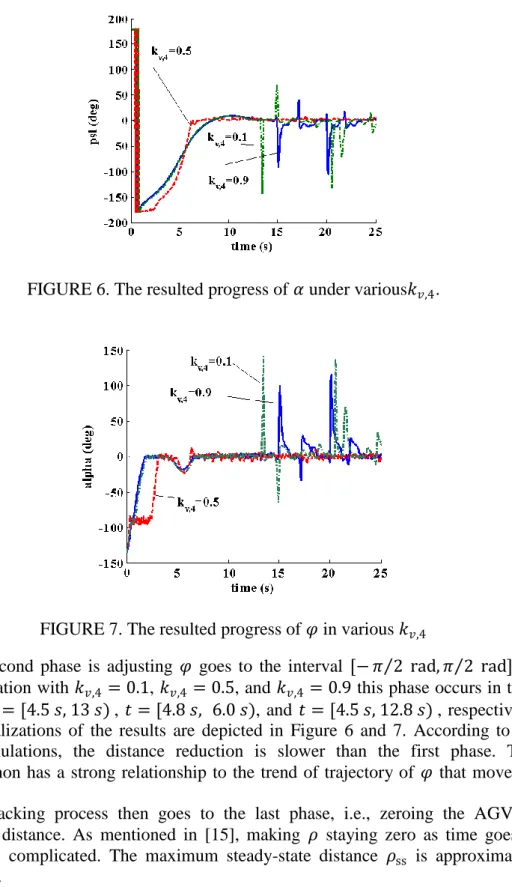
FIGURE 6. The resulted progress of 𝛼 under various𝑘𝑣,4.
FIGURE 7. The resulted progress of 𝜑 in various 𝑘𝑣,4
The second phase is adjusting 𝜑 goes to the interval [− 𝜋 2 rad, 𝜋 2 rad]. In the simulation with 𝑘𝑣,4 = 0.1, 𝑘𝑣,4 = 0.5, and 𝑘𝑣,4 = 0.9 this phase occurs in time
interval 𝑡 = [4.5 𝑠, 13 𝑠) , 𝑡 = [4.8 𝑠, 6.0 𝑠), and 𝑡 = [4.5 𝑠, 12.8 𝑠) , respectively. The visualizations of the results are depicted in Figure 6 and 7. According to the three simulations, the distance reduction is slower than the first phase. This phenomenon has a strong relationship to the trend of trajectory of 𝜑 that moves to zero.
The tracking process then goes to the last phase, i.e., zeroing the AGV-to-reference distance. As mentioned in [15], making 𝜌 staying zero as time goes to infinity is complicated. The maximum steady-state distance 𝜌ss is approximately 0.3-0.5 m.
5. CONCLUSIONS
A trajectory tracking control algorithm with AGV-reference distance paradigm for rear-steered AGV is proposed. The main purpose of the controller is to reduce
Computer Engineering and Applications Vol. 7, No. 2, June 2018
AGV-to-reference distance under the extreme initial navigation variables. Simulations show that the process of tracking consists of three phases: adjusting 𝛼 to zero followed by adjusting 𝜑 to zero, and finally make the AGV closer to its reference by driving 𝜌 closer to zero. This research is planned to continue to some aspects of this type of control, such as determining the maximum allowable time to drive the AGV to the maximum steady-state distance.
ACKNOWLEDGEMENTS
This work was supported by the institution’s research funds from Department of Industrial Engineering, Faculty of Industrial Engineering, Universitas Atma Jaya Yogyakarta, and Lembaga Penelitian dan Pengabdian pada Masyarakat (LPPM) Universitas Atma Jaya Yogyakarta.
REFERENCES
[1] M. ten Hompel and T. Schmidt, Warehouse Management: Automation and Organization of Warehouse and Order Picking Systems, Springer-Verlag Berlin Heidelberg, 2007.
[2] B.-I. Kim, S. S. Heragu, R. J. Graves, and A. S. Onge, “A Hybrid Scheduling and Control System Architecture for Warehouse Management”, IEEE Transactions on Robotics and Automation, Vol. 19, No. 6, pp. 991-1001, December 2003.
[3] X. Zhang, Y. Gong, S. Zhou, R. de Kostef, and S. van de Velde, “Increasing the Revenue of Self-Storage Warehouses by Optimizing Order Scheduling”,
European Journal of Operational Research, Vol. 252, No. 1, pp. 68-78, July 2016.
[4] W. Lu, D. McFarlane, V. Giannikas, and Q. Zhang, “An Algorithm for Dynamic Order-Picking in Warehouse Operations”, European Journal of Operational Research, Vol. 248, No. 1., pp. 107-122, January, 2016.
[5] A. P. Aguiar, J. P. Hespanha, and P. V. Kokotovic, “Path-Following for Nonminimum Phase Systems Removes Performance Limitations”, IEEE Transactions on Automatic Control, Vol. 20, No. 2., pp. 234-239, Februari 2005.
[6] T. A., Tamba, B. Hong, and K.-S. Hong, “A Path Following Control of An Unmanned Autonomous Forklift”, International Journal of Control, Automation, and Systems, Vol. 7, No. 1, pp. 113-122, March 2009.
[7] A. K. Pamosoaji and K.-S. Hong, “A Path-Planning Algorithm Using Vector Potential Functions in Triangular Regions”, IEEE Transactions on Systems, Man, and Cybernetics: Systems, Vol. 43, No. 4, pp. 832-842, July 2013.
[8] P. Coelho and U. Nunes, “Path-Following Control of Mobile AGVs in Presence of Uncertainties,” IEEE Transactions on AGV, vol. 21, no. 2, pp. 252-261, April 2005.
[9] L. Lapierre, R. Zapata and P. Lepinay, “Combined Path-Following and Obstacle Control of a Wheeled AGV,” International Journal of AGV Research, vol. 26, no. 4, pp. 361-375, April 2007.
[10] I. Zohar, A. Ailon, and R. Ravinovici, “Mobile Robot Characterized by Dynamic and Kinematic Equations and Actuator Dynamics: Trajectory Tracking and Related Application”, Robotics and Automation Systems, Vol. 59, No. 6, pp. 343-353, June 2011.
[11] J. Yuan, F. Sun, and Y. Huang, “Trajectory Generation and Tracking Control for Double-Steering Tractor-Trailer Mobile Robots with On-Axle Hitching”,
IEEE Transactions on Industrial Electronics, Vol. 62, No. 12, pp. 7665-7677, July 2015.
[12] M. Egerstedt, X. Hu, and A. Stotsky, “Control of Mobile Platforms Using a Virtual AGV Approach”, IEEE Transactions on Automatic Control, Vol. 46, No. 11, pp. 1777-1782, November 2001.
[13] D. Chwa, “Sliding-Mode Tracking Control of Nonholonomic Wheeled Mobile Robots in Polar Coordinates,” IEEE Transactions on Control Systems Technology, vol. 12, no. 4, pp. 637-644, July 2004.
[14] A. Widyotriatmo and K.-S. Hong, “Switching Algorithm for Robust Configuration Control of A Wheeled AGV”, Control Engineering Practice, Vol. 20, No. 3., pp 315-325, March 2012.
[15] A. Widyotriatmo and K.-S. Hong, “Asymptotic Stabilization of Nonlinear Systems with State Constraints”, International Journal of Applied Mathematics and Statistics, Vol. 53, No. 3, pp. 10-23, 2015.
[16] D. Chwa, “Tracking Control of Differential-Drive Wheeled Mobile Robots Using a Backstepping-Like Feedback Linearization”, IEEE Transactions on Systems, Man, and Cybernetics-Part A: Systems and Humans, Vol. 40, No. 6, pp. 1285-1295, November 2010.
[17] Z. Li, J. Deng, R. Lu, Y. Xu, J. Bai, and C.-Y. Su, “Trajectory-Tracking Control of Mobile Robot Systems Incorporating Neural-Dynamic Optimized Model Predictive Approach”, IEEE Transactions on Systems, Man, and Cybernetics: Systems, Vol. 46, No. 6, pp. 740-749, August 2015.
[18] E. Kayacan, H. Ramon, and W. Saeys, “Robust Trajectory Tracking Error Model-Based Predictive Control for Unmanned Ground AGVs”, IEEE/ASME Transactions on Mechatronics, Vol. 21, No. 2, pp. 806-814, October 2015