An online-integrated condition monitoring and prognostics framework for rotating equipment

(1)

CRANFIELD UNIVERSITY

LINDA ANTOUN YOUSEF ALRABADY

AN ONLINE-INTEGRATED CONDITION MONITORING AND

PROGNOSTICS FRAMEWORK FOR ROTATING EQUIPMENT

SCHOOL OF ENGINEERING

Department Of Power And Propulsion

This thesis is submitted in fulfilment of the requirements for the

degree of PhD In Mechanical Engineering

Academic Year: 2008 - 2014

Supervisor: Professor David Mba

October 2014

publication may be reproduced without the written permission of the

(2)

ABSTRACT

Detecting abnormal operating conditions, which will lead to faults developing later, has important economic implications for industries trying to meet their performance and production goals. It is unacceptable to wait for failures that have potential safety, environmental and financial consequences. Moving from a “reactive” strategy to a “proactive” strategy can improve critical equipment reliability and availability while constraining maintenance costs, reducing production deferrals and decreasing the need for spare parts. Once the fault initiates, predicting its progression and deterioration can enable timely interventions without risk to personnel safety or to equipment integrity.

This work presents an online-integrated condition monitoring and prognostics framework that addresses the above issues holistically. The proposed framework aligns fully with ISO 17359:2011 and derives from the I-P and P-F curve. Depending upon the running state of machine with respect to its I-P and P-F curve an algorithm will do one of the following:

(1) Predict the ideal behaviour and any departure from the normal operating envelope using a combination of Evolving Clustering Method (ECM), a normalised fuzzy weighted distance and tracking signal method.

(2) Identify the cause of the departure through an automated diagnostics system using a modified version of ECM for classification.

(3) Predict the short-term progression of fault using a modified version of the Dynamic Evolving Neuro-Fuzzy Inference System (DENFIS), called here MDENFIS and a tracking signal method.

(4) Predict the long term progression of fault (Prognostics) using a combination of Autoregressive Integrated Moving Average (ARIMA)- Empirical Mode Decomposition (EMD) for predicting the future input values and MDENFIS for predicting the long term progression of fault (output).

(3)

The proposed model was tested and compared against other models in the literature using benchmarks and field data. This work demonstrates four noticeable improvements over previous methods:

(1) Enhanced testing prediction accuracy, (2) comparable processing time if not better, (3) the ability to detect sudden changes in the process and finally (4) the ability to identify and isolate the problem source with high accuracy.

(4)

Keywords:

Condition Monitoring, Prognostics, Short Term Prediction, Long Term Prediction, Online, Automated Diagnostics, Clustering, Empirical Model Decomposition, Autoregressive Moving Average, Particle Swarm optimisation, Fuzzy Logic, Neural Network.

(5)

ACKNOWLEDGEMENTS

“I can do all things through him who strengthens me.” Philippians 4:13

I am thankful first and above all to my Lord, God almighty for his fulfilled promises and for always being there to strengthen me in the difficult times. Without him I can do nothing.

The current work is a result of assistance, guidance and support from several people. As such I would like to thank every one of them for his/her role in making this successful.

I would like to thank my supervisor Dr. Mba, who expertly guided me through all stages of my PhD. I am thankful for your advice, critical comments and support. I would like to also thank my husband and champion Yousef Rabadi to whom I owe alot, I can’t even start counting the blessings having you in my life. My sweet heart and bundle of Joy, Helen, Mum I pray that God will give me the power to raise you and see you successful in everything you do.

I am indebted to my parents, whose value to me grows with time. Mum and Dad I hope that this will make you proud of me, you were always in mind while working hard to complete this work with all the other responsibilities I had to manage too.

(6)

LIST OF FIGURES

Figure 2-1 Failure progression timeline (Vachtsevanos et al. 2007) ... 35

Figure 2-2 ISO 17359:2011 CBM Framework (BS ISO 17359:2011 2011) ... 36

Figure 2-3 Example Offline Data Collection and Validation ... 37

Figure 2-4 Fault Detection and Identification Process (Wegerich 2005) ... 49

Figure 2-5 Fault Classification Process Using BEMD and RVM (Tran et al. 2013) ... 53

Figure 2-6 C4.5 Decision Tree (Karabadji et al. 2014) ... 55

Figure 2-7 Feed Forward Neural Network ... 62

Figure 3-1 Single Layer Feed Forward Network ... 68

Figure 3-2 Neural Networks Classifications ... 69

Figure 3-3 Adaptive Network Legend ... 69

Figure 3-4 Single Layer Feed Forward Network Example ... 70

Figure 3-5 A Generalised Bell Shaped MF ... 71

Figure 3-6 A Generalised Bell-Shaped MF at Various Width Values ... 72

Figure 3-7 A Generalised Bell-Shaped MF at Various Slope Values ... 72

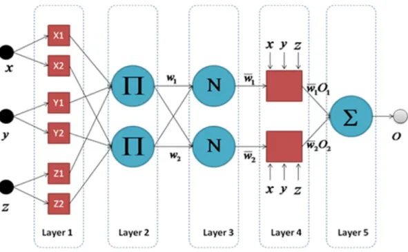
Figure 3-8 First Order TSK ANFIS Network ... 75

Figure 3-9 ANFIS Hybrid Learning Process ... 77

Figure 3-10 An Online ECM Process ... 81

Figure 3-11 Particle Swarm Optimisation Example ... 82

Figure 3-12 Auto-correlation and Partial Correlation Plots Example ... 88

Figure 3-13 End to End Process of EMD ... 91

Figure 3-14 Mackey Glass Time Series Plot ... 92

Figure 3-15: EMD for Mackey-Glass Time Series ... 93

Figure 3-16 Mackey-Glass Time Series Superimposed on the EMD output and the Error Difference ... 93

Figure 3-17 Tracking Signal Example ... 95

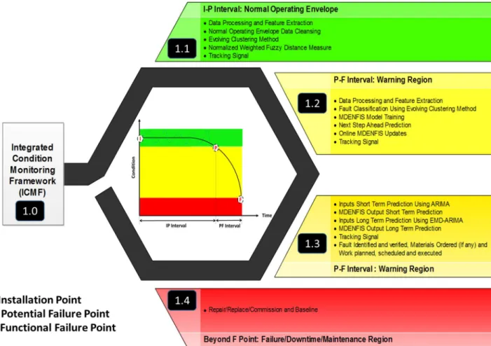
Figure 3-18 Integrated CM and Prognostics Framework ... 97

Figure 3-19 IP and PF Curve... 98

(10)

Figure 3-21 Normal Operating Envelope Region ... 102

Figure 3-22 Failure Modes versus Health Indicators Matrix ... 106

Figure 3-23 Warning Region Short Term Prediction ... 108

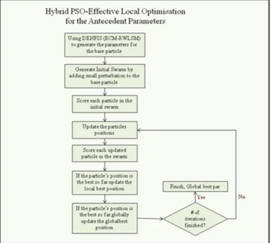
Figure 3-24 MDENFIS with PSO Global Optimisation ... 111

Figure 3-25 MPSO using Effective Local Approximation Method ... 112

Figure 3-26 Remaining Useful Life (RUL) Prediction ... 113

Figure 3-27 Warning Region Short Term and Long Term Prediction ... 114

Figure 3-28 Failure/Downtime/Maintenance Region ... 115

Figure 4-1 Time Series Analysis ... 116

Figure 4-2 Original and Smoothed Temperature Trends ... 117

Figure 4-3 Example Database Showing Outliers and NaNs ... 118

Figure 4-4 Temperature Trend Normalisation using Min-Max Method ... 119

Figure 4-5 Mackey-Glass Time Series ... 120

Figure 4-6 Gas Furnace Dataset Inputs/Output ... 121

Figure 4-7 Iris Dataset Inputs/Output Trends ... 122

Figure 4-8 Iris Setosa, Virginica and Versicolor Clusters (1-3) ... 122

Figure 4-9 CO2 Concentration Prediction One Step Ahead ... 126

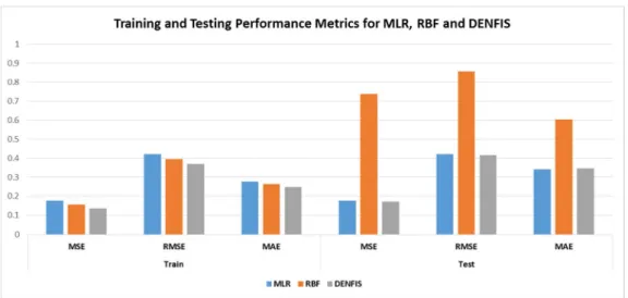
Figure 4-10 Training and Testing Performance Metrics for MLR, RBF and DENFIS ... 126

Figure 4-11 Mackey-Glass Dataset 1 Inputs/Output Trends... 131

Figure 4-12 Initial Number of Learning Inputs/Output Pairs Optimisation ... 131

Figure 4-13 Initial Number of data pairs Close to a Cluster Centre Optimisation ... 132

Figure 4-14 Initial Sigma Optimisation ... 132

Figure 4-15 Training and Testing NDEI Results ... 135

Figure 4-16 Training NDEI Trend Over 250 Generations of the MPSO ... 135

Figure 4-17 Original and Modified Cluster Centres ... 137

Figure 4-18 Original and Predicted Output at x(t+6) and the Testing Error .... 137

Figure 4-19: Gas Furnace Input Data Clustering Optimization ... 139

Figure 4-20: Gas Furnace Testing Results for DENFIS and MDENFIS (with and without online Updates) ... 140

(11)

Figure 4-21 Iris Testing Results Showing Two Misclassified Cases ... 143

Figure 4-22 Iris Testing Results 150/150 inputs/output pairs (11 Clusters) .... 144

Figure 4-23 120/30 Testing inputs/output pairs (12 Clusters) ... 144

Figure 5-1 Examples of Different Types of Compressors ... 148

Figure 5-2 Centrifugal Compressor Process Flow Levels ... 150

Figure 5-3 Centrifugal Compressor Main Components ... 151

Figure 5-4 Centrifugal Compressor Train Maintainable Items as per ISO 14224 ... 152

Figure 5-5 Generic Centrifugal Compressor Matrix Mapping Relationships between Failure Modes and Observed Effects ... 152

Figure 5-6 PF Curve for A specific Failure Mode ... 154

Figure 5-7 Example Discharge Pressure versus Flow Rate Curve ... 157

Figure 5-8 Example Polytropic Efficiency versus Flow Rate Curve ... 157

Figure 5-9 Example Polytropic Head versus Flow Rate Curve ... 158

Figure 5-10 Fouled Centrifugal Compressor Rotor ... 160

Figure 5-11 Fouled 1st_{Stage Discharge- Particulate Fouling ... 161}

Figure 5-12 Coking at the stage inlet ... 162

Figure 5-13 Impeller Corrosion and Return Bend Pitting ... 162

Figure 5-14 Centrifugal Compressor Polytropic Efficiency versus Flow Rate over 8 years ... 164

Figure 5-15: Boundary Definition- Compressors (ISO 14224:2006) ... 166

Figure 5-16: Polytropic Efficiency Map ... 168

Figure 5-17: Polytropic Head Map ... 169

Figure 5-18: Polytropic Efficiency Trend over time (Ideal) ... 169

Figure 5-19: Relative Efficiency Drop (for the ideal model creation) ... 170

Figure 5-20: Ideal Performance Data Used for Model Training ... 170

Figure 5-21: Ideal Performance Parameters Prediction 1 ... 171

Figure 5-22: Ideal Performance Parameters Prediction 2 ... 171

Figure 5-23: Ideal Performance Model Prediction 3 ... 172

Figure 5-24: Relative Efficiency Drop Actual and Ideal Prediction ... 173

(12)

Figure 5-26 Polytropic Efficiency Actual and Predicted Trends ... 174

Figure 5-27 Relative Head Drop Predicted and Actual Trends ... 175

Figure 5-28 Relative Efficiency Drop Predicted and Actual Trends ... 175

Figure 5-29 Error Performance Measure Comparison ... 176

Figure 5-30 Average Robustness Measure Comparison ... 176

Figure 5-31 Average Spillover Measure Comparison ... 177

Figure 5-32 Summary Performance Metrics Results ... 177

Figure 5-33 Diagnostics Accuracy Measure for the Transformers Faults ... 180

Figure 5-34 Transformers Testing Actual and Predicted Outputs... 180

Figure 5-35 Relative Efficiency Drop Over Time ... 182

Figure 5-36: Pressure Ratio, Temperature Ratio and Polytropic Exponent Trends ... 183

Figure 5-37 Training NDEI Changes over 100 Generations ... 185

Figure 5-38 One Step Ahead Prediction Results Using Test 1,2 and 3 ... 186

Figure 5-39 Zoomed Results Within the following (455 and 485 Steps) ... 186

Figure 5-40 Empirical Mode Decomposition Results for the Relative Efficiency Drop Trend ... 188

Figure 5-41 EMD Results for the Sum of the first 4 IMFs Including the Residual ... 188

Figure 5-42 Remaining Noise of the Relative Efficiency Drop ... 189

Figure 5-43 250 Step Ahead Prediction Using EMD-ARIMA-MDENFIS ... 189

Figure 6-1 Rotating Equipment Condition Monitoring Literature Review ... 191 Figure 6-2 Machinery Prognostics Related Publications in the Last 30 years 192

(13)

LIST OF TABLES

Table 2-1 Data Validation Classifications ... 40

Table 2-2 Data Validation Methods, Classification Type, Error and Example Cause ... 41

Table 2-3 Rotating and Reciprocating Equipment Vibration Limits ... 48

Table 4-1 Training and Testing Performance Metrics for MLR, RBF and DENFIS ... 127

Table 4-2 Mackey-Glass Dataset Testing NDEI and Training Time ... 128

Table 4-3 Testing NDEI and Training Time Comparison ... 128

Table 4-4 Number of Fuzzy Rules and Testing NDEI Comparison ... 129

Table 4-5 Comparison of Number of Rules, Testing NDEI and Training Time 133 Table 4-6 Number of Rules, Training and Testing NDEI Testing ... 136

Table 4-7 MSE, RMSE, NDEI and Number of rules for the training, Testing and Online Update- Testing Stages. ... 139

Table 4-8 Gas Furnace Dataset 2 Testing Comparison ... 141

Table 4-9 Iris Classification Using ECMcm and Neural Network Comparison 143 Table 4-10 Iris Testing Accuracy using Different Dataset Sizes ... 145

Table 5-1 Positive Displacement and Dynamic Compressors Main Characteristics ... 148

Table 5-2: Performance Model Parameters... 167

Table 5-3 Fault Codes and Their Distribution within the Dataset ... 179

Table 5-4 Faults Classification Accuracy Comparison ... 181

Table 5-5 Inputs Correlation Results with the Relative Efficiency Drop ... 183

(14)

LIST OF EQUATIONS

(2-1) ... 43 (2-2) ... 44 (2-3) ... 45 (2-4) ... 56 (3-1) ... 70 (3-2) ... 71 (3-3) ... 73 (3-4) ... 75 (3-5) ... 76 (3-6) ... 76 (3-7) ... 76 (3-8) ... 77 (3-9) ... 78 (3-10) ... 78 (3-11) ... 78 (3-12) ... 78 (3-13) ... 78 (3-14) ... 78 (3-15) ... 79 (3-16) ... 79 (3-17) ... 79 (3-18) ... 79 (3-19) ... 79 (3-20) ... 81 (3-21) ... 83 (3-22) ... 83 (3-23) ... 84 (3-24) ... 86

(15)

(3-25) ... 86 (3-26) ... 87 (3-27) ... 87 (3-28) ... 89 (3-29) ... 89 (3-30) ... 91 (3-31) ... 95 (3-32) ... 103 (3-33) ... 103 (3-34) ... 103 (3-35) ... 103 (3-36) ... 109 (3-37) ... 109 (3-38) ... 109 (3-39) ... 110 (3-40) ... 110 (4-1) ... 118 (4-2) ... 118 (4-3) ... 120 (4-4) ... 123 (4-5) ... 123 (4-6) ... 123 (4-7) ... 123 (4-8) ... 124 (4-9) ... 124 (4-10) ... 124 (5-1) ... 155 (5-2) ... 158 (5-3) ... 158

(16)

(5-4) ... 158 (5-5) ... 159 (5-6) ... 159 (5-7) ... 159 (5-8) ... 159 (5-9) ... 159

(17)

LIST OF ABBREVIATIONS

ANFIS Adaptive NeuroFuzzy Inference System AI Artificial Intelligence

AR Autoregressive

ARIMA Autoregressive Integrated Moving Average BPNN Back Propagation Neural Network

BARTFIS Bayesian ART-based Fuzzy Inference System BWR Benedict-Webb-Rubin

BEP Best Efficiency Point

BEMD Bi-dimensional Empirical Mode Decomposition BS-EMD B-Spline Empirical Mode Decomposition BIT Built-in Test

CART Classification And Regression Tree CBM Condition Based Maintenance CM Condition Monitoring

ECMc Constrained Evolving Clustering Method CHC Convex Hull Classifier

CF Crest Factor DAQ Data Acquisition

DPNN Deep Belief Neural Network DGA Dissolved Gas Analysis

DWNN Dynamic (Recurrent) Wavelet Neural Networks DENFIS Dynamic Evolving NeuroFuzzy Inference System ELAM Effective Local Approximation Method

EMD Empirical Modes Decomposition

EEMD Ensemble Empirical Model Decomposition ETTF Estimated Time to Failure

ECM Evolving Clustering Method EFuNN Evolving Fuzzy Neural Networks ESOM Evolving Self-organising Maps eTS Evolving Takagi Sugeno EWN Evolving Wavelet Network

(18)

FMECA Failure Modes Effects and Criticality Analysis

FAOS-PFNN

Fast and Accurate Online self-organizing scheme for Parsimonious Fuzzy Neural Networks

FFT Fast Fourier Transformation

FFNN Feed Forward (Static) Neural Network FEM Finite Element Method

FEC Fuzzy Entropy Clustering Method FIS Fuzzy Inference System

FL Fuzzy Logic

GDFNN Generalised Dynamic Fuzzy Neural Network GRNN Generalized Regression Neural Network GA Genetic Algorithms

HMM Hidden Markov Model

ICMF Integrated Condition Monitoring Framework IMFs Intrinsic Mode Functions

LDC Linear Discriminant Classifier

LOWESS Locally Weighted Scatter Plot Smoothing MTS Mahalanobis Taguchi System

MAD Mean Absolute Deviation MSE Mean Square Error MTBF Mean Time to Failure MFs Membership Functions

MDENFIS Modified Dynamic Evolving NeuroFuzzy Inference System MPSO Modified Particle Swarm Optimisation Method

MA Moving Average

MIMO Multi-Inputs Multi-Outputs MISO Multi-Inputs Single Output MLP Multilayer Perceptron MLR Multiple Linear Regression

MSET Multivariate State Estimation Technique NaN Not a Number

NF NeuroFuzzy Models

NDEI Non-Dimensional Error Index NOE Normal Operating Envelope

(19)

OEM Original Equipment Manufacturer PD Partial Discharge

PSO Particle Swarm Optimisation pk-pk Peak to Peak

PCA Principal Component Analysis PNN Probabilistic Neural Network QDC Quadratic Discriminant Class RBF Radial Basis Function

RNN Recirculation Neural Network RVM Relevance Vector Machine RAN Resource-Allocating Network RCFA Root Cause Failure Analysis RMS Root Mean Square

RMSE Root Mean Square Error SOM Self-Organising Maps

STFT Short Time Fourier Transformation SMEs Subject Matter Experts

SVM Supper Vector Machine TSK Takagi-Sugeno-Kang WPT Wavelet Packet Transform WT Wavelet Transform

0-pk Zero to Peak

WPT-EMD

(20)

1 INTRODUCTION

1.1 Overview

The history of Maintenance goes back even to the time of the ancient Egyptians 5000 years ago when they built an extraordinary and enduring civilisation culminating in the great pyramids. Even after this long time they are still standing there to remind us of the highly refined skills that were utilised to build them and the care that was given through the periodic inspections to every part of them. Even in more recent times, simple but effective method of using a canary as a sensor for detecting the existence of gas contaminations in the air was utilised in the coal mining industry. Since the canaries are very sensitive to the quality of air, they will lose consciousness even with low concentration of toxic or hazardous gases like carbon monoxide and methane, miners used them as gas detectors - as long as the birds are alert, the air is fresh. Otherwise a bird losing consciousness indicates immediate response such as evacuation for the whole mine due to air contamination.

In modern commercial production industry, the trend is increasing towards the need for high availability equipment which are working 24/7. This means that any failure, even if minor, is unwanted due to its production and economic impact. Maintenance techniques involve applying one or more methods to restore equipment serviceability or to ensure equipment remains operational to the required performance. The following types of techniques may be used:

 Detection

(21)

 Repair/restore

 Exchange

 Re-design

The increased complexity and criticality of equipment over the years has resulted in a drastic change in the way owners used to monitor, maintain and repair their equipment.

Pre 1950’s one of the main maintenance methods used was what is called “Corrective Maintenance “. This type of maintenance is carried out when a failure occurs. Other names for it include "run to failure" or "break down maintenance". There are three significant drawbacks from only utilising this maintenance method:

 Safety of workers: certain failures are catastrophic and may cause death to workers.

 Production related: due to the unexpected nature of these failures in terms of time and the lead time needed to order and replace parts which in some cases might take weeks if not months.

 Environmental related

Preventive maintenance was used in WWII and before – even the Romans had an upkeep by exchange scheme for their armies hardware (effectively planned maintenance), and Condition Monitoring was used by "wheel tappers" on Railways 150 years ago.

Preventive Maintenance is mainly a time or cycle-based method where certain inspections and PMs are scheduled at certain frequencies to be conducted. For

(22)

example: bearing replacement every 2 years, oil changes every year or based on the number of working hrs or cycles, etc. Usually these tasks are based on many factors like the original equipment manufacturer’s recommendations referenced in the equipment maintenance manual and sometimes based on experience. Although preventive maintenance promises to solve many of the problems caused by adapting wrong maintenance practises like corrective maintenance through reducing the number of unplanned shutdowns however it doesn't eliminate these failures completely and there are always occasions which result in the requirement for corrective maintenance. In addition, this type of maintenance can be very costly, in terms of replacing components before their end of useful life, and necessitates keeping huge inventory of components which are needed in case of failure and most important wasting resources. Preventive maintenance only applies to age-related failure modes, and has little or no effect on improving availability on other failure modes (random failure modes).

In recent times, industry has moved to applying condition based (or predictive) approach to maintenance based on trending and analysing the data from one or more parameters which indicate the presence or development of known failure modes and fault conditions. This is managed by collecting data like process parameters (temperature, pressure, flow rate, power consumption, etc.) And other health indicators like Vibration, Noise, Current signature, etc. (Jardine et al. 2006).

Analysis of this data helps in assessing the overall health of equipment and it is then possible to plan required maintenance based on the severity of the detected fault (Vachtsevanos et al. 2007), equipment condition and its criticality to the

(23)

production line. Condition based maintenance can be effective for most failure modes, including age related and random.

Researchers in conjunction with industry have started to focus on this type of maintenance (Predictive Maintenance) to enhance its deliverables through utilising different techniques of measurement and signal processing, fusing data from different sources to reduce the uncertainties related to human and instrumentations errors,…etc. In modern days there has been a trend towards automating the whole process. That leads to the desire of the engineering management and planners to have information such as the estimated useful life of their equipment and the ability of the equipment to perform the required tasks until the next planned shutdown successfully. This involves diagnostics and prognostics and results in optimisation of maintenance planning and cost. The rapid growth of Maintenance Methods from Corrective Maintenance (Run until shutdown) through Preventive (Time based) to Predictive Maintenance (Condition based) decreased the trends of unplanned shutdown events and production deferrals.

This avoids supporting the cost of huge amount of spare parts inventory and enables proper planning for spare parts ordering, taking into consideration the machine condition and the lead time of delivery of these replacement parts. Most important it improves the safety of personnel as a result of avoiding unmonitored catastrophic failures of machinery.

(24)

The advancements in the areas of data collection, signal processing, transducers technologies and continuous improvement of diagnostic and prognostic models have enabled the development of the CBM approach.

1.2 Problem Statement

Rotating equipment are considered the backbone and major component of any oil and gas plant. Like any other type of equipment, these equipment are designed to run for many years trouble-free, however in reality, there is a difference between the equipment designed Mean Time to Failure (MTBF) and the actual MTBF due to many factors including but not limited to: poor design, wrong assembly and installation, running the equipment at extreme operating and environmental conditions, etc. 80% of rotating equipment failures are random (meaning that there is no obvious relation between how long the equipment has been in service and the likelihood of failure happening) as compared to 20% aged related failures however rotating equipment have distinctive characteristics that can be monitored and analysed to give an indication about their overall health. Moving from a “reactive” maintenance strategy to a “proactive” maintenance strategy can improve critical equipment reliability and availability while constraining maintenance costs, reducing production deferrals and decreasing the need for spare parts. In support of a proactive maintenance strategy, condition monitoring has gained a lot of interest from researchers and industries. Many developments and novelty approaches were presented, applied and proven to have excellent outcomes. However majority of these approaches rely heavily on human expertise, as people move on, the knowledge moves with them creating sustainability issues when applying these approaches adding to that the

(25)

likelihood of human errors. As a result, an increasing trend towards automating the process was seen in recent years. Detecting abnormal operating conditions, which will lead to faults developing later, has important economic implications for industries trying to meet their performance and production goals. It is unacceptable to wait for failures that have potential safety, environmental and financial consequences to happen. Once the fault initiates, predicting its progression and deterioration can enable timely interventions without any risk to personnel safety or to equipment integrity.

This prediction can help in two sides: check whether the equipment will survive until the next planned shutdown and check the remaining useful life of the equipment also called prognostics. The short and long term predictions are normally calculated using the present and past equipment health taking into consideration any variations in the operating conditions in the past, present and future. During the life cycle of the equipment some routine maintenance tasks may help improving the overall health of the equipment like for example applying lubrication to bearings regularly while some others can potentially have an adverse effect on the overall health of the equipment again using the previous example if the routine task is done in the wrong way by over greasing a bearing, this put the bearing under too much stress and eventually cause a bearing failure. It’s important to be able to detect these sudden changes in the process and act accordingly. To enable an informed maintenance planning for the work to be done rather than by trial and error which will definitely extend the downtime duration, the type of failure mode needs to be identified either through an automated or manual process. Subject Matter Experts are normally involved either ways.

(26)

Different models were applied for diagnostics and prediction purposes ranging from statistical and reliability models, physical based models, data driven models and hybrids of more than one model. Majority of the work done assumed that the data is available upfront to train, validate and test the proposed models when in reality this isn’t the case for example: with a newly installed equipment there is no historical data available. As such an online model is needed that updates itself continuously with any newly acquired data/knowledge. This is a very important feature to apply the model across both new and old equipment, to avoid limitations in previous models caused by data availability which cover a wide range of normal and faulty operating conditions but most important to detect transient changes resulting from instrumentation errors, actual maintenance/repair events, etc. This work presents an online-integrated condition monitoring and prognostics framework that addresses the above issues holistically.

1.3 Scope of Research

Even though the proposed approach is applicable to any type of equipment (rotating, reciprocating and static), this work only looks at rotating equipment and implements the proposed model on a fouled centrifugal compressor.

Within the condition based maintenance framework, this work covers three main parts:

 Monitoring the departure of the equipment health indicators outside their normal operating envelope.

 Isolate and identify the fault developed through an automated diagnostics system

(27)

 Predict the future progression of the fault both short term and long term (prognostics)

There are some commonalities between the algorithms used for the above three tasks, due to the flexibility of the proposed model and its wide applications in the fields of prediction and classification.

The proposed model is a hybrid between two data driven techniques, namely: Neural Networks and Fuzzy Logic. This is supported by a global optimisation method (Modified Particle Swarm Optimisation) for fine tuning the solution obtained by the online grid partitioning method (Evolving Clustering Method). For both short and long term predictions, there are two scenarios. The first scenario assumes that the future inputs to the model are available and as such the model can be used for single step ahead and multi-step ahead predictions. The second scenario assumes that the future inputs to the model aren’t available, in real field applications this is normally the case. In the second scenario, a method is required to predict the future values of the inputs based on their past and present values, for this purpose a hybrid between the empirical mode decomposition and autoregressive moving average methods is proposed. The ECM for classification modified algorithm is proposed for the automated diagnostics task.

Even though the proposed approach is applicable to any type of equipment (rotating, reciprocating and static), this work only looks at rotating equipment and implements the proposed model on a fouled centrifugal compressor.

Within the condition based maintenance framework, this work covers three main parts:

(28)

 Monitoring the departure of the equipment health indicators outside their normal operating envelope.

 Isolate and identify the fault developed through an automated diagnostics system

 Predict the future progression of the fault both short term and long term (prognostics)

There are some commonalities between the algorithms used for the above three tasks, due to the flexibility of the proposed model and its wide applications in the fields of prediction and classification.

The proposed model is a hybrid between two data driven techniques, namely: Neural Networks and Fuzzy Logic. This is supported by a global optimisation method (Modified Particle Swarm Optimisation) for fine tuning the solution obtained by the online grid partitioning method (Evolving Clustering Method). For both short and long term predictions, there are two scenarios. The first scenario assumes that the future inputs to the model are available and as such the model can be used for single step ahead and multi-step ahead predictions. The second scenario assumes that the future inputs to the model aren’t available, in real field applications this is normally the case. In the second scenario, a method is required to predict the future values of the inputs based on their past and present values, for this purpose a hybrid between the empirical mode decomposition and autoregressive moving average methods is proposed. The ECM for classification modified algorithm is proposed for the automated diagnostics task.

(29)

1.4 Research Hypothesis

The research hypothesis are as follow:

1. The following modifications in the original DENFIS model can improve the model prediction accuracy: Using all generated rules, using exponential MFs instead of rectangular MFs. The null hypothesis is that the new proposed approach will make no difference or actually adversely affect the accuracy of the model.

2. A modified global optimisation method (MPSO) integrated with the proposed model can improve both the prediction accuracy and processing time of the model. The null hypothesis is that the new approach will make no difference.

3. Modifying the original model to learn/add new rules while working online can improve the models’ capabilities in detecting sudden changes in the process. The null hypothesis is that this modification will have no effect and the model won’t be able to detect sudden changes in the process. 4. Modifying the original model during the classification testing phase can

improve the classification accuracy of the model. The null hypothesis is that the new approach will make no difference.

1.5 Originality and Contribution

This work presents a novel approach in the following areas:

1. Proposing a hybrid of ECM and normalised weighted fuzzy distance for the first time to monitor where the machine is running with respect to its normal operating envelope (NOE) and then alert the user if departure outside this zone occurs by using a tracking signal. The combination of

(30)

ECM and weighted fuzzy distance is in its own a new model and also the usage of this model for predicting the normal equipment behaviour and compare that with where it’s actually running is a second contribution here. The process is proposed to be monitored using a tracking signal which has the capability of identifying any departure beyond the NOE.

2. Modifying the ECM for classification algorithm to enable online updating of the clusters during the testing stage. This feature enhanced the classification accuracy of 150 cases of the Iris flower from 98.6% to 100%. 3. Enhancing the prediction accuracy of the Dynamic Evolving NeuroFuzzy

Inference model by introducing the following changes to the model: using exponential membership functions instead of the originally proposed rectangular membership functions, integrating the model with a modified version of particle swarm optimisation to optimise the position of the clusters centres and width of the membership functions, and finally adding an online updating feature during the testing stage online to enhance the models capability of detecting sudden changes in the process.

4. Introducing a hybrid EMD-ARIMA model to enable predicting the future values of the inputs which in turn enables prediction of multiple steps ahead (long term prediction) of the health indicators. This modification was successfully tested on fouling progression rate and the model predicted successfully 250 days steps ahead.

1.6 Thesis Structure

This thesis consists of 6 main chapters. Chapter 1 gives an introduction to the research, research motivation, scope of research and main contributions. A

(31)

summary of an extensive literature survey conducted in the field of condition monitoring and prognostics is presented in Chapter 2. Chapter 3 covers the enabling technologies and theories, the proposed model is also described in details in this chapter. The proposed model was first tested on three benchmark datasets through 5 case studies to test a number of hypothesis for improvement in the prediction accuracy, processing time and classification accuracy in Chapter 4. This is then followed by validating the proposed model using field data for fouled compressor and electric transformers in Chapter 5.

Conclusions and recommendations are presented in Chapter 6. This chapter summarises the conclusions in light of the benchmarks and field datasets simulations, list the main contributions and proposes some future work.

(32)

2 LITERATURE SURVEY

2.1 An Introduction to Condition Based Maintenance (CBM)

CBM is a maintenance strategy whereby equipment is maintained according to its condition, rather than on an elapsed time or running hour’s basis. This strategy involves periodically analysing the equipment condition monitoring information like vibration, oil analysis, thermography, process data, etc. to assess its overall condition and to only carryout maintenance when required. The two main pillars of condition based maintenance strategy are diagnostics and prognostics. Diagnostics involves identifying the root cause of a problem whereby the problem has already occurred and Prognostics involves predicting the future health of the equipment either before or after a problem occurred (Jardine et al. 2006).

The implementation of any CBM strategy consists of four different phases: 1. Data collection: Data are normally acquired using online or offline condition monitoring systems. The two basic types of data are events and condition monitoring data (Jardine et al. 2006). Events data include equipment historical maintenance records and reliability information, and condition monitoring data include vibration, performance and process data, current signature analysis, oil analysis, etc. To ensure a successful CBM strategy both event and condition monitoring data should be used as they both have the same level of importance. The decision into which technology to use and at what measurement frequency is based on the failure modes likely to happen, their estimated time to failure (ETTF) and sensitivity of the condition monitoring parameters in detecting these failure modes.

2. Data analysis: Data collected are normally in raw format and might need cleaning, processing and potentially data reduction before any informed decision can be made based on this data. Cleaning involves removing wrongly assigned failure modes to certain events data, removing NaNs (Not a Number Values) and bad data. Advanced statistical and signal processing techniques can also be used to extract useful information from the data that are otherwise hidden within.

(33)

3. Decision Making: Once the data is processed and analysed the next step is to make a decision into the overall health of the equipment. This might involve an intrusive or nonintrusive actions. For instance, if the data indicates a machine running outside its normal operating envelope this could be as simple as recommending a change in its operating routines, whereas a late stage of fault development might involve a downtime to repair/replace the component involved. 4. Feedback: Once the maintenance action/change in the operating routines is taken it is vital to feedback any findings which will aid in the continuous improvement cycle of the CBM strategy.

2.1.1 Diagnostics

The foundation of any CBM strategy is robust and reliable fault diagnostic capabilities. Diagnostics algorithms are designed to assess equipment performance, monitor deterioration rates, and identify any impending failures based on certain parameters variations (Vachtsevanos et al. 2007). Ideally, such algorithms has the capability of identifying even the sub-equipment component that is failing and its failure mechanism. Over the last 50 years, an accelerating rate of publications in this area was noticed, recognising the importance of this pillar to any CBM strategy and trying to enhance its capabilities.

Some of the earliest fault diagnostic capabilities developed in the form of built-in test (BIT) for early generation aircrafts (Vachtsevanos et al. 2007). Continuous developments in the computer power and data storage capabilities and technology in general had a major influence on the accelerating trend of development in systems diagnostics capabilities as new information are made available. It is now possible to identify at an early stage the presence of incipient faults early enough to take action which could potentially reverse the failure progression process. Such capabilities enabled maintenance personnel to avoid potentially catastrophic failures and enhance the equipment reliability and availability.

(34)

2.1.2 Prognostics

Prognostics derives from the Greek word Prognostikos and means fore-knowing or fore-seeing, originally used in the Medical field by doctors to predict the chances that a patient will recover from a particular disease or that the disease will return back, by using statistical analysis methods based on groups of people whom suffer from same symptoms as that of this patient such that a proper treatment plan can be prepared. Due to the criticality and benefits of such kind of analysis for the Medical field the development of prognostics in the Medical field is more mature compared to other Industrial related applications (Absolute Astronomy 2009).

BS ISO 13381-1:2004 defines prognostics as: “the estimation of time to failure

and risk for one or more existing and future failure modes” (ISO 13381-1:2004

2004). This definition introduces the need for knowing the possible failure modes associated with the system or component under study through conducting Failure Modes and Effect Analysis (FMEA) study as outlined in IEC 60812 (IEC 60812 2006) or Failure Modes Effects and Criticality Analysis (FMECA) study as outlined in BS 5760-5 (BS 5760-5:1991 1991). The casual tree relationships between past, present and future failure modes is also described in this standard, differentiating between primary, secondary and tertiary failure modes. The secondary failure mode is the failure mode initiated due to an existing primary failure mode which influences this initiation and same for the tertiary failure modes. The physics of failure mechanisms forms one of the elementary parts of any successful Diagnostics/Prognostics framework (ISO 13381-1:2004 2004). Reference (Vachtsevanos et al. 2007) described that as the “cornerstone”. By conducting a FMECA study one can relate the failures/defects to their root cause i.e. failure mechanism.

Prognostics studies have been applied to different fields and different mechanical, electrical and electronic components and systems. Applications like: Rotating and reciprocating machinery from civil and military applications, batteries, circuit boards, specific components (bearings, gearboxes, etc.).

(35)

To maximise the benefits of a truly CBM strategy, additional capabilities, beyond the realm of diagnostics are required. Prognostics capabilities are designed to provide maintenance personnel with insight into the future health of a monitored equipment. Figure 2-1 illustrates the life cycle of an equipment from as new condition to a failed state (Vachtsevanos et al. 2007).

At the start of the equipment life cycle, the equipment is considered new, this could also be following completion of a work order and commissioning the equipment, successful transition from the infant mortality period, the equipment will continue in good working condition. After some time, an incipient fault condition develops in one of the equipment components. As time progresses, the severity of the fault increases until the component eventually fails, this is normally called the PF interval which is the time interval between the initiation of a potential fault in the component/equipment and the time component/equipment reaches its functional failure. If the equipment is allowed to continue operating beyond this point secondary and tertiary damage to other components will occur.

Diagnostics is normally done anytime between the very early incipient fault point and the sub-component functional failure depending on the sensitivity of the diagnostics system and/or competency of the analyst. However, prognostics can be done even prior to the initiation of the fault by detecting any early departure from the normal operating envelope. Prognostics has the potential to deliver major benefits as part of the CBM strategy more than any other maintenance approach by increasing the availability of the equipment and reducing the overall maintenance cost.

(36)

Figure 2-1 Failure progression timeline (Vachtsevanos et al. 2007)

There are different classifications for the diagnostics and prognostics methods in the literature, some are more general than the others. However, the three main approaches are (Heng et al. 2009), (Jardine et al. 2006):

 Model-based approaches: These approaches use physical principles and system identification methods in describing the failure initiation and growth. Due to the nature of these methods, the amount of data required with these models are minimal when compared with other approaches. However they are computationally expensive, fault specific, and not practical to be implemented on a larger scale.

 Data-driven approaches: These approaches depend on CM and other operational data collected to build the models. The accuracy of the output is very much linked to the amount and quality of collected data. Statistical Methods, Artificial Intelligence (AI), etc. belong to this approach.

 Hybrid approaches: These approaches combine either data driven and model based approaches and/or more than one data driven approach. The

(37)

objective is to improve the capabilities of the original models by combining more than one of them together to take advantage of the benefits of each of them. This approach has been adopted by the author and used through this thesis.

2.2 Condition Based Maintenance Framework

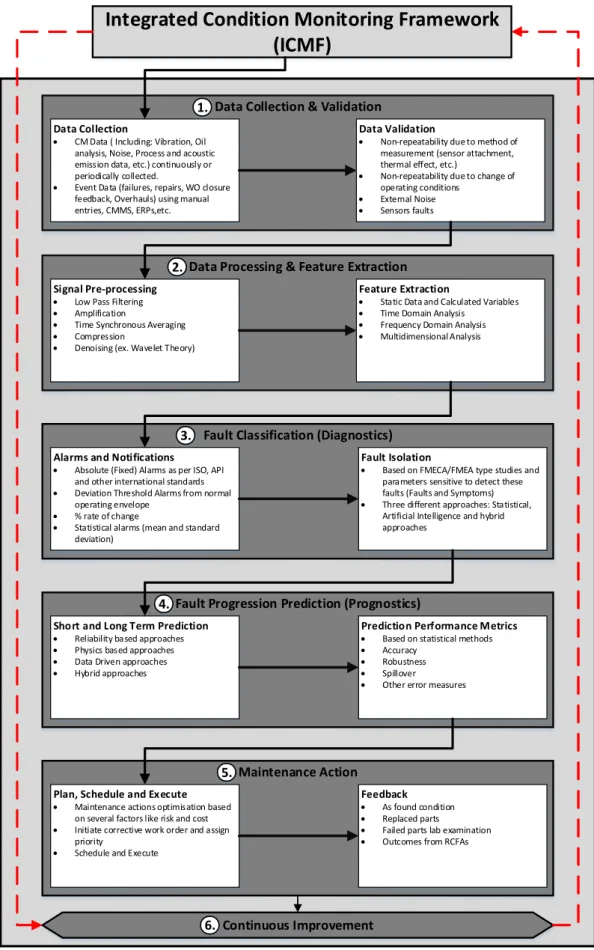
Figure 2-2 presents a CBM framework as proposed by ISO 17359:2011 (BS ISO 17359:2011 2011) where each stage performs a unique function to ensure the process of CBM can be successfully implemented.

Figure 2-2 ISO 17359:2011 CBM Framework (BS ISO 17359:2011 2011)

(38)

2.2.1 Data Collection and Validation

2.2.1.1 Data Collection

The process of acquiring various equipment parameters and storing them in a central database is called Data Collection (Jardine et al. 2006). Data is normally acquired from sensors placed on the equipment either permanently or temporarily to monitor certain aspects of the mechanical and performance behaviour of the equipment. An example offline data collection and validation process is shown in Figure 2-3, a vibration sensor monitoring the relative shaft vibration at a centrifugal compressor drive end bearing side is shown, the data is transferred through the cable to a data collection portable where data is stored temporarily until they get transferred to a desktop application for further validation and analysis.

Figure 2-3 Example Offline Data Collection and Validation

This data usually falls into two categories: condition monitoring (CM) and event data (Jardine et al. 2006). Examples of CM data are vibration, oil analysis, pressure, temperature, flow rate, valve opening position, etc. Examples of event data are information obtained from maintenance overhauls, routine preventive maintenance, visual inspection, etc. CM data can be classified based on the type of data acquired into static data like pressure and temperature readings and

(39)

dynamic data like vibration and noise time waveforms. Static data are normally trended over time and signs of departure from the normal operating envelope are normally captured through some predefined alarm limits either based on original equipment manufacturer’s recommendations, internationally accepted standards and/or based on subject matter experts experience. Dynamic data are normally collected at a specific time, this data are usually stored in a raw form which normally require further processing, like for example transformation into the frequency domain, extracting some statistical indicators like the mean, maximum and minimum values, etc.

Data collection can be done using either online or offline monitoring system. The two main differences are related to whether the data collection process is automatic or manual and whether data is collected from permanently installed or temporarily installed sensors.

In an online monitoring system, data is collected from permanently installed sensors on the equipment at various locations, ex. Vibration, bearing metal temperature, suction pressure , discharge pressure, suction temperature, and discharge temperature, fluid (or gas) flow rate, valve opening position, filter differential pressure, lube oil temperature and pressure, etc.. This data is collected automatically at a preconfigured sampling rate ranging from real-time continuous to periodic data collection. The preconfigured sampling rate is linked to time (ex. every 10 min, hourly, daily, etc.) or an event (ex. start-up/shutdown and also if an alarm limit is exceeded). Usually critical equipment like power generation and gas compression units are equipped with online monitoring systems.

In an offline monitoring system, data is collected from permanently or temporarily installed sensors on the equipment at various locations. This data is collected manually and periodically. The decision to monitor a piece of equipment with an offline monitoring system is based on a feasibility and cost justification study, taking into consideration criticality of equipment, the failure modes likely to occur and their lead time to failure but most importantly, the consequence of failure. Sometimes it isn’t even required to sample certain parameter continuously. Visual

(40)

Inspection and event data collection belongs to the offline monitoring category even though it’s not intrusive meaning that no sensors are required to be installed; it relies on the human senses. Infact this is the most commonly used offline monitoring technique in industry for all types and criticality of equipment. For all offline monitoring systems the measurement locations should be clearly identified and marked to ensure measurement repeatability

Data acquisition in its own will provide the raw data without any additional processing, however to enable a proper decision making relying on the diagnostics and prognostics outcomes, the data will almost always require further processing as raw data can include outliers, noise, nonstationary behaviour and others (Jablonski and Barszcz 2013). Using unclean data will affect the performance and quality of the overall process.

2.2.1.2 Data Validation

Whether data is collected using an online or offline monitoring system, it is vital to ensure that this data is validated before any informed decision can be made. Problems like electric interference, sudden changes in the process, sensor field wirings integrity, wrongly mounted sensors, etc. are some examples of issues that produce invalid readings (Jablonski and Barszcz 2013). Data validation in condition monitoring is the process of checking for errors in the collected data and correcting them (by replacing them, eliminate them from the analysis or mark them as invalid) to ensure high quality information are being fed to the following steps of the condition monitoring program. The objective is to only pass on complete, correct and consistent data. Data Validation is used in so many different fields (for example electrical engineering, chemical and petroleum engineering, computer science and information technologies, mechanical engineering, etc.) with various proposed methods that are applicable to some or all fields. A comprehensive literature survey into the topic is covered in (Sun, S. et al. 2011) with bias towards water systems. This survey classified data validation in 4 different ways as shown in Table 2-1:

(41)

Table 2-1 Data Validation Classifications

Class 1 Class 2 Class 3 Class 4

Manual Offline Simple tests Single dimensional

Automatic Online Physical/mathematical tests

Multi-dimensional

The first two classifications (Class 1 & 2) are linked to the data collection method whether this is online or offline. The need for automatic and online data validation methods has increased over the past decade with the increasing and dynamic developments nature of technologies and moving towards real time data collection methods where processing time is crucial. Within the condition monitoring umbrella, critical rotating equipment are normally equipped with online monitoring system to collect several condition monitoring indicators including vibration, bearing metal temperature, inlet and outlet pressures and temperatures, flow rate, etc. This is normally done at high sampling rate approaching real-time data collection.

Class 3 is based on the type of test used for data validation ranging from simple tests as simple as visual examination of the data in a trend plot or using some graphical applications and as complex as using certain mathematical tests like principle component analysis and artificial neural networks.

Class 4 is based on the type of data, whether this is Univariate (single dimensional) or multivariate (dimensional). In Data validation for multi-dimensional dataset the interaction between the different variables is normally studied and any abnormal behaviour is flagged. Data validation isn’t going to be described in more details in the section as it isn’t the main topic of the author’s research however a comprehensive review is provided in Table 2-2 which include commonly used methods of data validation in the literature, their classification based on Classification III in Table 2-2, errors and example causes.

(42)

Table 2-2 Data Validation Methods, Classification Type, Error and Example Cause

Method Classification Type Error Example Cause References

Status Check Simple test Working Staus Cabling shorts, open circuits, Power supply failure

na Calibration Due Date Check Simple test Calibration Status Out of Date Calibration for an accelerometer na Drift detection by exponentially

weighted moving averages

physical or mathematical tests Drifts slowly evolving, gradual faults (Ross et al. 2012), (Millioz et al. 2011)

Signal's gradient test Simple test Drifts Loose connections, sensor saturation, sudden change of load

(Jablonski and Barszcz 2013), (Pouliezos and Stavrakankis 1994)

Constant Value Detection Simple test Flatlined Trend Data Loss (Jablonski and Barszcz 2013)

Presence Check Simple test Missing Data Intermittent data feed disconnection (D 3.1.1)

Limit Check (Physical Range, Local realistic range and tolerance band)

Simple test Outliers Incorrect probe sensitivity used, sensor settings, unit conversions

(Kim et al. 1992),(Gryllias and Antoniadis 2012)

Extreme Value Check Using Statistics physical or mathematical tests Outliers Loose connections, sensor saturation, sudden change of load

(D 3.1.1) Multivariate statistical test using PCA or

kernal PCA

physical or mathematical tests Outliers air sample contamination (Gribok et al. 2000), (Brown et al. 2010),(Dunia et al. 1996) Data Mining Technology physical or mathematical tests Outliers and other

quality issues

Various sensors issues (D 3.1.1)

Gross Error Detection physical or mathematical tests Outliers zero error (imperfect calibration of sensors), environmental changes, imperfect

measurement process

(Qin and Li 1999)

Uncertainity Considerations physical or mathematical tests Uncertainity Measurement uncertainities (D 3.1.1) Material Redundancy Detection Simple test lack of redundancy damaged sensor or gradual performance

deterioration

(D 3.1.1) Spatial consistency Method physical or mathematical tests Uncorrelated damaged sensor or gradual performance

deterioration

(Lee 1994) Analytical redundancy Method physical or mathematical tests Uncorrelated damaged sensor or gradual performance

deterioration

(43)

2.2.2 Data Processing and Feature Extraction

This process involves three different phases: feature extraction, data cleaning and feature selection. Data cleaning can be done prior to the features extraction in the collected raw data domain or after extracting the features. It is important though to ensure that only clean data is passed on to the next stage which involves fault classification and diagnostics. These three phases are introduced one by one below.

2.2.2.1 Feature Extraction

In most cases, raw data cannot be used directly for diagnostic and prognostic purposes. One needs a way of obtaining useful information from the raw data; this is known as feature extraction. The useful information extracted is often referred to as the condition indicators or features; they reflect the health status of the equipment or component. Around 99% of all failures are preceded by changes in one or more health indicators (Geitner and Bloch 2012). Feature extraction is a widely studied problem for which numerous models, algorithms and tools have been developed. These are reviewed in terms of their domain here. The collected raw time waveform data can be directly analysed in the time domain by extracting useful characteristic information (features) from the signal using statistical methods. The following are examples of some extracted features: peak amplitude or zero to peak (0-pk), peak to peak (pk-pk), root mean square (RMS), Crest Factor (CF), variance and standard deviation, other higher statistical orders, etc. The definition of these extracted features is given in (Sun et al. 2004). CF is calculated using the ratio between the 0-pk and RMS values of the time waveform, it gives a good representation about the presence of impacts in the time waveform, this is especially of great importance as a health indicator for rolling element bearings. Kurtosis is based on a comparison between the 4th statistical moment and the second statistical moment squared as shown in equation 2-1. It gives an assessment about how the data is distributed around the mean value.

(44)

(2-1)

In (Samanta and Nataraj 2008) the kurtosis feature was used as a condition indicator for the prognosis of gearbox condition subject to gear pitting wear. Time domain features can also be extracted using more complex statistical models. In (Samuel and Pines 2005) a comparison was made between several time domain features and their sensitivity in detecting faults of helicopter gearboxes. In (Poyhonen et al. 2004) an autoregressive model was built based on vibration data collected from a motor, the parameters of the model were used condition indicators (features) for fault identification. Other parametric time series applications can be found in (Mechefske and Mathew 1992) and (Baillie and Mathew 1996).

A time waveform is a mixture of one or more frequencies which make the signal too complicated to be analysed in the time domain. Transforming this data into a different domain might be a better option in this case. Every fault has a characteristic frequency that identifies it. Transforming the data from the time to the frequency domain will highlight all the frequencies contributing to the complex time waveform shape. Those frequencies can then be compared to the main faulty frequencies for fault identification purposes. The most popular time to frequency domain transformation technique is the Fast Fourier Transformation (FFT), however this method only applies to stationary time waveforms (constant mean and variance) else signal processing errors might be generated. Other widely used techniques are: enveloping (Stack et al. 2002), power spectral density, etc.

With some of the developed faults the stationary assumption of the time waveform isn’t any more valid hence a third hybrid domain of the two was proposed in the literature to address this issue namely the Time-Frequency domain analysis. The most typical method of this kind is wavelet transform (WT).

(45)

WT has developed rapidly in the recent decades and has been widely used for feature extraction (Mori et al. 1996), (Yang et al. 1999), (Staszewski et al. 1999) and (Cheung et al. 1993). A continuous WT is described by equation 2-2 below:

(2-2)

Where:

( ) is the time waveform, is the scale parameter, is the time parameter and is the WT function

Widely used WT techniques include continuous WT, discrete WT (Mori et al. 1996), (Wu and Hsu 2009), (Wu and Liu 2008) and (Wu and Kuo 2009), and wavelet packet transform (WPT) (He and Shi 2002). (He and Shi 2002) Applied a Time-Frequency domain method (WPT) to extract faulty valves features from the vibration data collected at a number of reciprocating pumps. (Saravanan and Ramachandran 2009) Extracted certain features using various wavelets for bevel gearbox failure modes classification. (Wang et al. 2010) Developed a continuous wavelet transform based approach for fault detection under variant loads. Short Time Fourier Transformation (STFT) was develop to address the nonstationary signal issue by introducing a sliding FFT window over the signal, assuming that within this window the part of the signal analysed is stationary (Gao and Yan 2006).

In (Forrester 1989a), (Forrester 1989b) and (Forrester 1989c) Wigner Ville Distribution was applied to vibration data from transmission gears for faults (ex. cracked tooth and pitting) detection.

Empirical Mode Decomposition (EMD) as a novelty time-frequency domain method was first introduced in (Huang 1999). As the name reflects, the signal is decomposed into a number of signals and a residual signal. The decomposed signals are called intrinsic mode functions (IMFs). The major IMFs are normally used for feature extraction. EMD and AR were used in (Cheng and Yang 2006)

(46)

for extracting features from vibration data of roller element bearings for diagnostics purposes.

2.2.2.2 Data Cleaning

In certain cases, the extracted features using the time, frequency and time-frequency domain method are not 100% reliable and need to be further processed in order to identify and eliminate any unwanted outliers. This is known as data cleaning. This stage involves two successive actions, detecting and eliminating outliers. The key problem in data cleaning is how to accurately detect existing outliers. Classical methods of detecting outliers adopt a statistical way where some distance measure is used to find out the similarity between a particular data point and the rest of the data. The Mahalanobis distance described by equation 2-3 is an example of distance measures used for outliers detection in the multidimensional space:

(2-3)

where is a random vector, representing attributes or features in N dimensional space, the mean value is µ, and the covariance matrix is S . The MD considers the correlation between different features.

(Rousseeuw and Zomeren 1990) Proposed to compute a distance measure derived from the covariance of data points and their robust locations estimates. (Fung 1999) Proposed a method of detecting outliers based on the S-estimation robust method. (Shieh and Hung 2009) Proposed a method for detecting outliers in microarray data using Principal Component Analysis (PCA) and Mahalanobis Distance. Other methods like: Low Pass Filtering, Time Synchronous Averaging (Coats et al. 2009) and Adaptive Noise Cancellation (Chhikara and Singh 2012) were used in the literature for data cleaning.

2.2.2.3 Features Selection

Generally speaking, feature selection for classification and diagnostics purposes is different from that for prediction and prognostics purposes. For prognostics, researchers focus mainly on Univariate time series prediction where only one

(47)

feature is involved, so suitable features can be directly selected by visualizing their trends, e.g. if the values for a feature monotonically increase as time passes, this feature could be a good representative of the overall health of the equipment. For diagnostics, the rationale behind feature selection is more complex for classification problems where the dimension of features space is usually greater than one. For a certain problem, many recommended features may be extracted according to the reported literature; however, these features may not all be useful since practical cases vary with specific assumptions, constraints, etc. For cases where all features are required and the number of features is small, one can simply use all of them, but if the dimension of feature space is enormous, there will be a huge computational burden for the forthcoming stage, classification. It is, however, more common for some features to be redundant and/or irrelevant. The redundant features contribute nothing to the classification results but the feature space size, and any irrelevant features actually adversely affect the classification results; hence, such features should be selected and eliminated from the feature space.

Selection methods are generally classified into filters and wrappers. The main difference between the two is that with filters, the feature selection process is done in isolation of the learning algorithm used whereas with wrappers the leaning algorithm is included as part of the selection process (Kohavi 1995) and (Kohavi and John 1996), wrappers normally give better accuracy however on the expense of computational time. Principal Component Analysis (Malhi and Gao 2004), ranking variables based on their correlation coefficient values (Thiry et al. 2004), Support Vector Machines (Weston et al. 2001), (Chapelle et al. 2001) and (Yang et al. 2014) and decision tree algorithms (Kohavi and John 1996) are some examples of feature selection methods.

2.2.3 Fault Classification (Diagnostics)

Diagnostics is defined as the identification and isolation of a fault condition. Many approaches were published in the literature for diagnostics and classification problems. Example review papers for diagnostics approaches can be found in (Korbicz et al. 2004), (Jardine et al. 2006) and (Vachtsevanos et al. 2007). Two

(48)

main steps are normally covered within this area: 1. Identify the overall health status, i.e. machine in alarm or not and 2. Isolate the fault type and location. Both will be described in more details below.

2.2.3.1 Alarms and Notifications

Alarms represent a departure of equipment condition outside its normal operating envelope. This can be in the form of absolute alarms, residuals, step change, narrow band alarms and statistical alarms. Table 2-3 shows a list of rotating and reciprocating equipment covered by ISO 10816 and ISO 7919 specifically for absolute and relative shaft vibration severity limits. These limits are normally used as a guide if the Original Equipment Manufacturer (OEM) limits aren’t defined or specified.

Setting up residual alarms based o