Logistic Model Tree Extraction From
Artificial Neural Networks
Darren Dancey, Zuhair A. Bandar, and David McLean
Abstract—Artificial neural networks (ANNs) are a powerful and widely used pattern recognition technique. However, they remain “black boxes” giving no explanation for the decisions they make. This paper presents a new algorithm for extracting a logistic model tree (LMT) from a neural network, which gives a symbolic rep-resentation of the knowledge hidden within the ANN. Landwehr’s LMTs are based on standard decision trees, but the terminal nodes are replaced with logistic regression functions. This paper reports the results of an empirical evaluation that compares the new deci-sion tree extraction algorithm with Quinlan’s C4.5 and ExTree. The evaluation used 12 standard benchmark datasets from the University of California, Irvine machine-learning repository. The results of this evaluation demonstrate that the new algorithm produces decision trees that have higher accuracy and higher fidelity than decision trees created by both C4.5 and ExTree.
Index Terms—Artificial intelligence, feedforward neural net-works, multilayer perceptrons (MPLs), neural networks.
I. INTRODUCTION
A
RTIFICIAL neural networks (ANNs) are universal ap-proximators and, therefore, can approximate any Borel measurable function to an arbitrary accuracy [1]. For classi-fication, this means that neural networks can easily solve any practical classification problem [2] and have been successfully applied to a diverse range of problem domains. For example, recent applications have included problems from financial [3], engineering [4], and medical [5] domains.However, despite their relative success, the further adoption of neural networks in some areas has been impeded due to their inability to explain, in a comprehensible form, how they have made a decision. This lack of transparency in the neural network’s reasoning has been termed the Black Box problem. Andrewset al.[6] observed that ANNs must obtain the capabil-ity to explain their decisions in a human-comprehensible form before they can gain widespread user acceptance and to enhance their overall utility as learning and generalization tools.
Neural networks store their “knowledge” in a series of real-valued weight matrices representing a combination of nonlin-ear transforms from an input space to an output space. Rule extraction attempts to translate this numerically stored knowl-edge into a symbolic form that can be readily comprehended. The ability to extract symbolic knowledge has many potential advantages: the knowledge obtained from the neural network
Manuscript received December 21, 2005; revised June 28, 2006. This paper was recommended by Associate Editor J. Basak.
The authors are with the Department of Computing and Mathematics, Manchester Metropolitan University, Manchester, U.K. (e-mail: d.dancey@ mmu.ac.uk).
Digital Object Identifier 10.1109/TSMCB.2007.895334
can lead to new insights into patterns and dependencies within the data; from symbolic knowledge, it is easier to see which features of the data are the most important; and the explanation of a decision is essential for many applications, such as safety-critical systems.
Andrewset al.[6] and Tickleet al.[7], [8] summarize several proposed approaches to rule extraction. Many of the earlier approaches required specialized neural network architectures or training schemes. This limited their applicability; in particular, they cannot be applied to in situ neural networks. The other approach is to view the extraction process as a learning task. This approach does not examine the weight matrices directly but tries to approximate the neural network by learning its input–output mappings.
An example of this second approach has been to extract decision trees from the neural network [9]–[11]. Decision trees [12], [13] are a graphical representation of a decision process. The combination of symbolic information and graphical pre-sentation make decision trees one of the most comprehensible representations of pattern recognition knowledge. However, decision trees are a more limited form of classifier than neural networks [14]. This paper presents a new rule extraction method that extracts a logistic model tree (LMT) from a trained neural network. LMTs [15] are a recent addition to decision trees that replace the terminal nodes of a decision tree with logistic regression functions. This has the advantage of producing deci-sion trees that are more comprehensible, have higher accuracy, and have higher fidelity with the neural network than previous decision tree extraction algorithms.
This paper is organized as follows. The next section recaps the pattern classification problem and some relevant techniques used to solve it. Section III overviews rule extraction and important previous rule extraction methods. Section IV de-scribes ExLMT, which is our new rule extraction method. In Section V, ExLMT is empirically evaluated on a number of standard benchmark datasets from the University of California, Irvine (UCI) machine-learning repository. Sections VI and VII provide the discussion and the conclusion, respectively.
II. PATTERNCLASSIFICATION
The basic framework for classification [2] is that objects need to be classified as coming from a number of classes C1, . . . , CK. A process called feature extraction takes a number
of measurementspfrom the object. This produces a vector of featuresXcommonly called an instance.X, therefore, belongs to an instance space X =X1× X2× · · · × Xp, where Xi is either the set of real numbers for continuous valued features 1083-4419/$25.00 © 2007 IEEE
or a finite set for nominal valued features. The task is then to build a classifierˆcthat, given an instance,X =x, will classify it as belonging to one of theKclasses, i.e.,
ˆ
c:X → {1,2, . . . , K}. (1) To estimateˆc, a training setT must be available that consists of a series of instances augmented with a known classification. These example instances with known classification can then be used to estimate the parameters inˆc.
Neural networks are one method of implementing such a classifier. ExLMT also makes use of decision trees and logistic regression to implement classifiers, and these three methods will be briefly described next.
1) Neural Networks: The field of neural networks consists of a large collection of models and techniques origi-nally inspired by biological nervous systems, such as the human brain [16], [17]. The basic building block of neural networks is the artificial neuron [18]. These artificial neurons accept a number of weighted inputs then process these inputs to produce an output. It is the value of these weights that determine the function mapping of the neural network. Using the backpropagation algorithm [19], multiple layers of perceptrons organized into a network are able to learn nonlinear mappings such as the pattern recognition task of (1).
2) Decision Trees: Decision trees [12], [13] are one of the most widely used classifier models. They are di-rected acyclic graphs consisting of nodes and connections (edges) that illustrate decision rules. Each nonterminal node has a splitting test associated with it, which splits the data into mutually exclusive subsets. The terminal nodes called leaves represent a classification. This has the effect of partitioning the instance spaceXinto a series of disjoint regionsRseparated by axis-parallel hyperplanes
X =
r∈R
Xr,Xr∩ Xr
=∅, where Xr=Xr. (2)
3) Logistic Regression: Logistic regression [20] is a statis-tical method used to predict posterior-class probabilities P(C=k|X =x)for theKclasses. Logistic regression fornvariables fits a logistic function of the form
y= e β0+n 1βixi 1 +eβ0+ n 1βixi (3) to the class probabilities, whereβiare the parameters to
be most commonly estimated using maximum-likelihood estimation.
III. RULEEXTRACTION
Rule extraction from neural networks aims to reduce the complexity of a neural network into a more easily understood symbolic form. These rules can then be analyzed for trustwor-thiness for safety-critical systems or used to provide insights into the relationships found by the neural network.
Andrewset al.[6] classifies rule extraction algorithms along the following five dimensions:
1) expressive power; 2) translucency;
3) specialized training regimes; 4) quality of the extracted rules; 5) algorithmic complexity.
The expressive power refers to the type of rules extracted from the neural network. Previous rule extraction techniques have extracted rules expressed in various form including Boolean logic [21], fuzzy logic [22], IF . . . THEN . . . rules [23], n-of-mrules [24], and decision trees [9], [10].
The Translucency means the level of granularity with which the neural network is examined. Craven and Shavlik [9] divided these into decompositional techniques, which examined the individual weights, and pedagogical techniques, which treated the neural network as a black box and learns the concept represented by the neural network by using it as an oracle.
Many of the rule extraction algorithms require the standard neural network training algorithms, such as backpropagation, to be modified. Although such techniques have been successful, they tend not to be portable across different neural network types. Andrewset al.[6] proposes four metrics for measuring the quality of the rules extracted from the neural network: accuracy, fidelity, consistency, and comprehensibility. Accuracy measures the ability of the rule set to correctly classify previ-ously unseen instances from the problem domain, i.e.,
P(ˆc(X) =C). (4) Fidelity is how well the extracted classifier (ˆc) corresponds to the original neural network (nn). It can be stated as the probability
P(ˆc(X) =nn(X)). (5) Consistency, in this context, is whether the extracted rule set is the same under different training sessions of the neural network. Comprehensibility is a measure of the number of rules produced by the extraction algorithm. The final dimension is algorithmic complexity, which attempts to provide a measure of the efficiency of the technique, considering such aspects as whether the algorithm scales exponentially with the number of hidden nodes or inputs.
A. Existing Extraction Methods
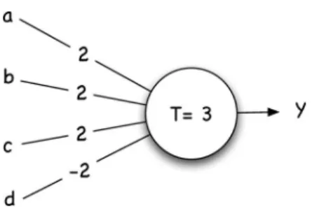
The subset rule extraction method [23] is typical of the decompositional approach, and similar methods have been pro-posed by Saito and Nakano [25] and Fu [21]. The subset method extracts a series of rules from each node in the network. A rule is created for each combination (or subset) of inputs that could cause a node to activate. For example, given the node in Fig. 1, the following rules could be extracted:a∧b∧c=⇒ y,a∧b∧ ¬d=⇒y,a∧c∧ ¬d=⇒y,b∧c∧ ¬d=⇒y,b∧ c∧ ¬d=⇒y. This particular implementation requires the
Fig. 1. Neural node with four inputs and a threshold value of three.
outputs of the nodes to be binary and, therefore, cannot be applied to preexisting multilayer perceptrons (MLPs) that nor-mally have nodes with real valued outputs. Moreover, the number of rules increases exponentially with the number of nodes, making the algorithm intractable for large networks. This approach was extended by then-of-m method, again by Towell and Shavlik [23]. A n-of-m rule contains a set m of tests, of whichnmust be satisfied for the rule to be evaluated as true. For example, then-of-mrule 2-of-{r1, r2, r3}is equiv-alent to (r1∧r2)∨(r1∧r3)∨(r2∧r3). This style of rule is particularly appropriate for representing the activation of a neural node. For example, the rules of Fig. 1 can be represented as 3-of-{a, b, c,¬d}. However, for a multiple-layered network to be represented in a concise number ofn-of-mrules and over-come the exponential growth problem of the subset algorithm, the antecedents of the rules should be equivalent, i.e., it does not matter whichnistrue. Standard backpropagation has no predisposition to favor such an arrangement. Therefore, either the neural network needs to be initialized using a preexisting rule set and/or trained using a special training algorithm.
Algorithms [26], [27] have been proposed which extract fuzzy rule sets [28] from neural networks. These approaches usually require a domain expert to label the resulting fuzzy sets and/or require specialized neural network architectures and training algorithms. These approaches have generally been applied to rule refinement, where a preexisting set of fuzzy rules have their membership functions refined by the neural network. Jang and Sun [29] have noted a functional equivalence between radial basis function networks and fuzzy inference systems under some conditions. However, it has been shown that the equivalence conditions are more restrictive than was initially thought, resulting in special training algorithms again being required [30].
Trepan [31] follows the pedagogical approach to rule ex-traction. Trepan creates an n-of-m decision tree [32], which, in addition to the C4.5-style splitting rule, can make use of an n-of-m splitting rule at any of the nodes. The use of n -of-msplits can fit certain concepts more naturally than C4.5-style splits at the cost of a certain amount of comprehensibility. Another interesting feature of Trepan is its use of best first tree expansion in contrast to the more usual depth-first expansion. The next node to expand is the node that maximizes the function
n∗= arg max
n (reach(n) (1−fidelity(n))) (6)
where reach(n) is the number of instances that have reached nodenand fidelity(n)is the percentage of instances at noden that the decision tree and the neural network are classified as the same class. This has the effect of concentrating growth of the tree in the region that increases fidelity the most. However, after the tree is fully grown and pruned, the difference between the two methods is negligible. But, the real advantage of this approach is the ability to more precisely control the accuracy growth tradeoff. To decide which attribute to base the splitting test on, Trepan uses information gain. To extract the “knowl-edge” from the neural network, Trepan uses a sampling-and-querying approach. The neural network is used as an oracle, which can be queried for the class assignment of a sampled instance. To create a query instance, Trepan models the original dataset using an empirical distribution for nominal attributes and kernel density estimation [33] for the continuous attributes. The empirical distribution means that the nominal values are sampled with a probability based on their frequency in the original dataset. For the continuous attributes, a probability-density function (PDF), using a kernel probability-density estimate with a Gaussian kernel, is sampled.
ExTree [10] creates a tree using the more comprehensible C4.5-style splitting rules. Unlike Trepan, ExTree uses a simple depth-first tree expansion scheme, resulting in large trees that overfit the data. A similar method to that employed in Quinlan’s C4.5 algorithm is then used to prune the tree.
ExTree uses a slightly modified version of information-gain ratio, which is a modification to information information-gain that compensates for multiway splits. ExTree, like Trepan, samples from empirical distributions for nominal attributes and a kernel density estimate of the PDF for the continuous attributes.
A further advantage of the pedagogical approaches is that they can be applied to any “black-box” classifier, such as ensembles of neural networks [34].
IV. EXLMT
This section describes ExLMT, a new method of extracting an LMT from a neural network. Current decision tree extraction methods such as Trepan and ExTree have produced reason-able results on many datasets, but there remains a significant gap between the accuracy of the neural network and the ex-tracted decision tree. This clearly indicates that more infor-mation remains to be extracted. Moreover, on many datasets, the extracted decision trees and the neural network disagree on the classification on a significant number of instances (low fidelity).
ExLMT extracts a form of LMT from the neural network. The LMT method is a recent contribution to the machine-learning field [15]. Decision trees produced by LMT are similar to standard decision trees but have the terminal nodes replaced by a polytomous logistic regression model. The replacement of the terminal nodes by logistic models has two significant effects: The decision tree now predicts class probabilities in-stead of giving a simple class assignment and the nodes are linear combinations of a subset of the attributes resulting in decision hyperplanes that are not axis-parallel. Fig. 2 shows how a two LMT tree may fit a 2-D instances space. Fig. 3 gives
Fig. 2. Decision hyperplanes of an LMT tree. Instances inside the gray box are of class 1. Instances outside the box are of class 2. The solid axis-parallel lines show the C4.5-style splitting rules, and the dotted lines show the nonaxis parallel splits achievable by using the logistic regression nodes.
an overview of the ExLMT algorithm. Each of the component steps will now be expanded.
Step 1) Acquire or train the neural network: before the ExLMT can be used to build a decision tree, a trained neural network is required. The ExTree method, being a pedagogical type of rule extraction, is independent of the neural network architecture and training algorithm.
Step 2) Relabel the dateset:recall that the original training setT consisted of the instanceXand a known clas-sificationC. A new relabeled datasetRis created replacing the known classification with the mapping of the neural networkcˆ, such that
R={X,ˆc(X)}. (7) Step 3) Generate new data: ExLMT uses Craven’s sampling-and-querying approach [31] to elicit knowledge from the neural network. ExLMT models the original dataset then samples this model to create new instances. These new instances are then used to query the neural network, obtaining class labels. This has the effect of expanding the original dataset. To model the nominal attributes, an empirical dis-tribution is used. This means that nominal values in the new instances are sampled according to their frequency in the original dataset. For continuous attributes, a PDF is estimated using kernel density estimation with a Gaussian kernel
f(x) = 1 m m i 1 √ 2πσe−( x−ui 2σ )2 (8) where m is the number of original instances, ui
is the attribute value for the ith examples, and σ is the width for the Gaussian kernel. As illustrated in Fig. 4, the kernel density estimation can be thought of as creating a PDF by summing a series of Gaussian functions centered on the current data
Fig. 3. Outline of the ExLMT algorithm.
Fig. 5. LogitBoost: an adaptive Newton algorithm.
points with a standard deviation, or bandwidth, de-termined by the size of the dataset. Based on some preliminary experiments, ExLMT uses a bandwidth of 1/√m. The new instances’ attribute values are then sampled from this PDF. The new instancesT∗ are then labeled by the neural network to produce a set of instances to be added to the relabeled dataset
R, such that
T=R ∪ T∗. (9)
The next three steps create the LMT tree follow-ing the procedure given by Landwehr [15]. Nodes continue to be split while they contain at least ten instances or all the instances belong to the same class.
Step 4) Create initial logistic regression model:an initial logistic regression model is built using all the data in
T. The logistic regression model is then fitted using
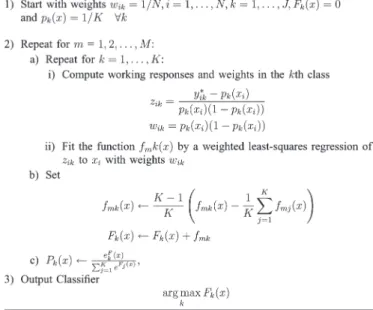
the LogitBoost method [35]. LogitBoost uses a en-semble of functions Fk to predict classes 1, . . . , K
using M “weak learners.” Fig. 5 details the Logit-Boost algorithm as originally given by Friedman.
Fk(x) = K m=1
fmk(x) (10)
Each of the “weak learners” fmk can be any
algo-rithm that fulfils (1). Whenfmkare linear functions
inx, thenFmk is equivalent to the logistic model.
The LogitBoost algorithm can then be seen as an iterative Newton method of fitting the logistic re-gression function.
Step 5) Create candidate splits:when deciding which at-tribute to split on, ExLMT considers two types of splitting rules. For discrete features, ExLMT creates a branch for each possible value of the feature. For real valued features, a binary split is made with two
outcomes Xi ≤α and Xi> α. To determine the
threshold value α, the set of instances are sorted on the value of feature Xi. An ordered set of m
instances can be divided into two ordered subsets m−1ways. ExLMT considers each of thesem−1 ways to divide the data for each of the real-valued features.
Step 6) Select best split: the previous step resulted in set of z candidate splitting tests,{T1, T2, . . . , Tz}; ExLMT uses an information-gain ratio [12], an in-formation entropy-based method to choose among this candidate tests. The aim is to select the test, which gives the most information about the class of the instances. The information gained by an event occurring is inversely proportional to the probability of the event occurring. The information of an event E occurring can be defined as log2(1/p(E)) =
−log2(p(E)) bits. Thus, the average amount of information needed to classify a pattern in a set S can be calculated as info(S) =− K i=1 p(Ci) log2(p(Ci)) bits (11)
withP(Ci)being the probability of an instance in
setS being a member of classCi. The information
gained by splitting the data according to test T can be found by calculating the average amount of information needed to classify an instance be-fore splitting the data and subtracting the amount of information needed to classify an instance for each of the subsets created by the split. Therefore, for a test T which results in N subsets, the sum of the average information of the N subsets, S=
N i=1Si, is infoT(S) = n i=1 |Si| |S| ×info(Si)bits. (12) The total information gained by testTcan be calcu-lated as
gain(T) =info(S)−infoT(S). (13) Information gain has a natural bias toward selecting the test, which splits the data into many groups. To overcome this bias, the information gain is divided by the information gained by arbitrarily splitting the set into the same number of subsets as the test. The information gained by arbitrarily splitting a set S intoNsubsets is given by
split info(T) = N i=1 |Si| |S| ×log2 |Si| |S| . (14)
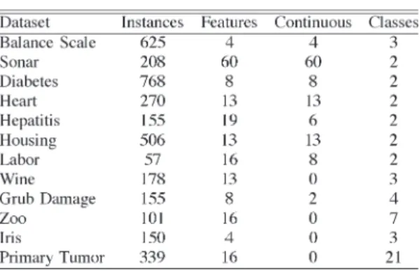
TABLE I DATASETCHARACTERISTICS
The gain ratio of testTcan, thus, be calculated as gain ratio(T) = gain(T)
split info(T). (15) ExLMT then uses the best splitT∗, which is the split that maximizes the information-gain ratio
T∗ = arg max
i (gainratio(Ti)). (16)
Step 7) Refine logistic model:for each node resulting from the split created at the previous stage, the logistic regression function is refined based only on the subset ofT that reached that node. This refinement means that, as the tree grows, the logistic regression models capture information local to the region ofX that the tree structure above has partitioned. Because of the iterative and additive nature of the LogitBoost algorithm, the refinement is simply running more iterations of a copy of the LogitBoost model of the node above but using only the subset ofT that reached this node.
V. EMPIRICALEVALUATION
ExLMT was evaluated using the criteria outlined in Section III on 12 standard benchmarking datasets from the well-known UCI machine-learning repository [36]. The pri-mary characteristics of the datasets are given in Table I.
The datasets represent a wide range of classification prob-lem domains. Because all the datasets, with the exception of balance-scale, are based on measured or observed data, they are likely to contain noise. Four of the datasets have only continu-ous features, and four datasets are purely nominal. The remain-ing eight datasets have a mixture of continuous and nominal features. Five of the datasets have more than two classes. The remaining seven datasets have a dichotomous class variable. Missing values in the datasets were replaced with the mean value of that feature. Other than this replacement, no other mod-ifications to the datasets were made. A stratified tenfold cross-validation [37] was carried out comparing ExLMT, ExTree, and C4.5. To further improve the reliability of the results, the
cross-validation was repeated ten times. A pairedt-test was used to test whether the difference between methods on each dataset was significant. Values whereP≤0.05were considered to be significant. To test whether the difference between the methods across the 12 datasets as a whole was significant, the Wilcoxon rank sign test was used. This test is similar to the well-known pairedt-test but does not make the assumption that the data are normally distributed. The null hypothesis for this test is that the two samples were drawn from identical populations, or from symmetric populations with the same mean. It is calculated by finding the differences between each matched pair, then ranking these differences by magnitude. The ranks are then labeled as negative if the difference was negative. The test statistic is then found by taking the smaller of theW+orW−, where
W+=(Positive Ranks) W−=
(Negative Ranks).
The W statistic is then evaluated against standard statistical tables to determine if it is significant.
A. Neural Network Parameters
To evaluate the rule extraction algorithms, neural networks with good predictive accuracy on the benchmark datasets were required. The neural networks were standard MLPs using back-propagation [19]. To avoid overfitting by the neural network, a momentum term was used [19]. The training algorithm min-imized the summed squared error with a weight decay term added, again to reduce the chance of overfitting. Given that the output of neural networks is y=f(x;w). The training examples are a set{xp,tp}. The error,Ebeing minimized by backpropagation, is then
E=
p
(tp−f(xp;w)p)2+ Φ
. (17)
Φis the decay term and is defined as the sum of the weightsw Φ =1
2
i
w2i (18)
where the sum runs over all the weights and biases.
Table II details the parameters used for the backpropagation algorithm for each dataset. The best parameters were chosen from a small selection of preliminary experiments, but further optimization of the parameters is likely to be possible. Epochs was the maximum number of iterations of the backpropagation algorithm. Validation size was the percentage ofT set aside to be used as a validation set. LR and MR are the learning and momentum rates, respectively. Decay refers to whether a decay term was used in the error function.
B. Results
Table III shows the average percentage accuracy of ExLMT compared to the original neural network, C4.5 and ExTree.
TABLE II
NEURALNETWORKPARAMETERS
TABLE III
CLASSIFICATIONACCURACY: MLP, C4.5,ANDEXTREE ANDEXLMT
TABLE IV
COMPARISON OFCLASSIFICATIONACCURACY: NUMBER OFTIMES
ALGORITHM INCOLUMNOUTPERFORMEDALGORITHM INROW
Table IV shows how the different methods compare with each other. Both tree-extraction techniques, ExTree and ExLMT, which extracted trees with higher accuracy than the C4.5-induced decision tree. ExLMT managed to extract de-cision trees that outperformed both C4.5 and ExTree trees on all 12 datasets. On one dataset (Iris), ExLMT extracted a decision tree with the same classification accuracy as the neural network. On seven of the datasets, ExLMT was within a percentage point of the accuracy of the neural network. Wilcoxon ranks sign tests showed that improvement in ac-curacy by ExLMT over C4.5 on the 12 datasets overall was significant(p= 0.0005). A further Wilcoxon test showed that the improvement of ExLMT over ExTree was also significant (p= 0.0005).
Table V shows the average fidelity of ExLMT with the neural network. The fidelity of C4.5 with the neural network was also calculated to give a baseline fidelity measure. Fidelity was
TABLE V
PERCENTAGEFIDELITY: C4.5, EXTREE,ANDLMT.∗t-TESTSHOWED
IMPROVEMENTAGAINSTC4.5 WASSIGNIFICANT
TABLE VI TREESIZE
calculated as the percentage of theminstances that a classifier, and the original neural network classified the same giving
fidelity(ˆc1,c2ˆ) = 1/m m i isEqual(ˆc1(xi),ˆc2(xi)) (19) where isEqual(a, b) = 1, a=b 0, a=b.
The fidelity of the ExLMT-extracted trees was compared to C4.5-induced trees and trees extracted using ExTree. Wilcoxon rank sign tests showed that the overall difference between ExLMT and both C4.5 and ExTree to be significant (p= 0.001, p= 0.002).t-tests showed that the difference on all but two datasets to be significant.
Table VI shows the average size of the tree produced by the three decision-tree algorithms.
VI. DISCUSSION
The results of the empirical evaluation showed that ExLMT-extracted trees have higher accuracy and fidelity than the Ex-Tree. This clearly demonstrates the advantage of the logistic models at the leaf nodes.
Interestingly, the fidelity on the Zoo and Iris datasets was lower with ExLMT than with the C4.5-produced decision tree.
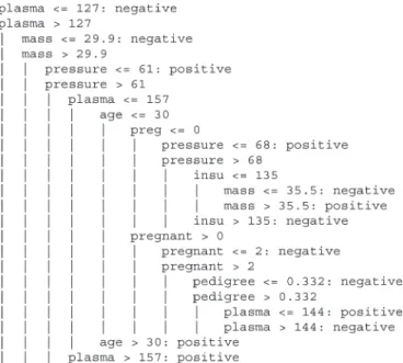
Fig. 6. C4.5-induced decision tree for the diabetes dataset.
However, the ExLMT-extracted tree, for these datasets, was significantly smaller than either the C4.5- or ExTree-produced trees. A possible explanation of this is that the simple logistic regression was a more appropriate model than a tree structure for these simple datasets.
A drawback of the original ExTree algorithm was that it produced trees with a large number of nodes, which reduces the comprehensibility of the model. ExLMT’s logistic model leaves are a much more compact representation but are less compre-hensible than the simple class assignment at the leaf node as used by C4.5 and ExTree. Although ExLMT produces trees with significantly less nodes than ExTree or even C4.5, whether these trees are more comprehensible overall is subjective.
If we consider two decision trees for the diabetes dataset, one induced using C4.5 (Fig. 6) and the other extracted from the ANN using ExLMT (Fig. 7). The C4.5 tree has 25 nodes, of which 13 are leaf nodes. In contrast, the ExLMT tree had only seven nodes, of which four were leaf nodes with logistic models. As shown previously in Table III, the ExLMT trees outperformed the C4.5 trees on this dataset. Both trees begin with a split on the plasma-glucose concentration level. This indicates that plasma is the most significant attribute. However, C4.5 and ExLMT differ in where the split point is made. C4.5 split at 127, which resulted in two subsets with 437 and 255 instances. ExLMT split at 139, which resulted in two subsets with 515 and 177 instances. The second level of the trees differ significantly. C4.5 chose to label the larger less-than-127 subset as negative for diabetes. Then, preceded to fur-ther partition the remaining instances with a 23-node subtree. Conversely, ExLMT did not split the higher than-139 group of instances instead assigning a single logistic model, Class0 = 15.49 − 0.13pregnant − 0.08plasma + 0.04pressure +
−0.02skin + −0.13mass + −2.49pedigree. This model had slightly higher accuracy and higher fidelity than the subtree and, in the opinion of the authors, is as comprehsible if not more so.
Fig. 7. ExLMT-extracted tree for the diabetes dataset.
VII. CONCLUSION
This paper has demonstrated a new method ExLMT, which is for extracting a decision tree from a trained neural network. An empirical evaluation was carried out comparing this new method to ExTree, a method that extracts traditional C4.5-style decision trees, and the C4.5 method that induced trees directly from the dataset. The evaluation was based on 12 well-known datasets from the UCI machine-learning repository. The evalu-ation showed that the extracted LMTs had significantly higher classification accuracy than either the corresponding C4.5 or ExTree trees. Additionally, on a majority of the datasets, the ExLMT-extracted trees had significantly higher fidelity with the neural networks than trees extracted using ExTree. ExLMT produced much smaller trees than either C4.5 or ExTree but, because of the additional logistic model at the leave nodes, it is unclear if these are easier to comprehend.
ACKNOWLEDGMENT
The authors would like to thank the anonymous referees for their insightful comments which helped to improve this paper.
REFERENCES
[1] K. Hornik, M. Stinchcombe, and H. White, “Multilayer feedforward networks are universal approximators,” Neural Netw., vol. 2, no. 5, pp. 359–366, 1989.
[2] B. D. Ripley,Pattern Recognition and Neural Networks. Cambridge, U.K.: Cambridge Univ. Press, 1996.
[3] P. C. Pendharkar, “A threshold-varying artificial neural network approach for classification and its application to bankruptcy prediction problem,”
Comput. Oper. Res., vol. 32, no. 10, pp. 2513–2522, 2005.
[4] K. M. Neaupane and S. H. Achet, “Use of backpropagation neural network for landslide monitoring: A case study in the higher Himalaya,”Eng. Geol., vol. 74, no. 3/4, pp. 213–226, 2004.
[5] C. M. Ennett, M. Frize, and E. Charette, “Improvement and automation of artificial neural networks to estimate medical outcomes,”Med. Eng. Phys., vol. 26, no. 3, pp. 321–328, 2004.
[6] R. Andrews, J. Diederich, and A. Tickle, “Survey and critique of tech-niques for extracting rules from trained artificial neural networks,”
[7] A. B. Tickle, R. Andrews, M. Golea, and J. Diederich, “The truth will come to light: Directions and challenges in extracting the knowledge embedded within trained artificial neural networks,”IEEE Trans. Neural Netw., vol. 9, no. 6, pp. 1057–1068, Nov. 1998.
[8] A. Tickle, F. Maire, G. Bologna, R. Andrews, and J. Diederich, “Lessons from past, current issues, and future research directions in extracting knowledge embedded in artificial neural networks,” inHybrid Neural Systems, S. Wermter and R. Sun, Eds. New York: Springer-Verlag, 2000. [9] M. W. Craven and J. W. Shavlik, “Extracting tree-structured representa-tions of trained networks,” inAdvances in Neural Information Processing Systems 8. Denver, CO: MIT Press, 1997, pp. 24–30.
[10] D. Dancey, D. Mclean, and Z. Bandar, “Extracting decision trees from trained artificial neural networks,” inProc. 17th Int. FLAIRS, 2004, pp. 515–519.
[11] A. Browne, B. D. Hudson, D. C. Whitley, M. G. Ford, and P. Picton, “Biological data mining with neural networks: Implementation and appli-cation of a flexible decision tree extraction algorithm to genomic problem domains,”Neurocomputing, vol. 57, pp. 275–293, 2004.
[12] J. R. Quinlan,C4.5 : Programs for Machine Learning. San Mateo, CA: Morgan Kaufmann, 1993.
[13] L. Breiman, J. H. Friedman, R. A. Olshen, and C. J. Stone,Classification and Regression Trees. New York: Chapman & Hall, 1984.
[14] D. Michie, D. J. Spiegelhalter, and C. C. Taylor,Machine Learning, Neural and Statistical Classification. New York: Ellis Horwood, 1994. [15] N. Landwehr, M. Hall, and E. Frank, “Logistic model trees,”Mach.
Learn., vol. 59, no. 1/2, pp. 161–205, May 2005.
[16] S. Haykin, Neural Networks: A Comprehensive Foundation, 2nd ed. Englewood Cliffs, NJ: Prentice-Hall, 1999.
[17] C. M. Bishop,Neural Networks for Pattern Recognition. Oxford, U.K.: Oxford Univ. Press, 1995.
[18] W. McCulloch and W. Pitts, “A logical calculus of the ideas immanent in nervous activity,”Bull. Math. Biophys., vol. 5, no. 4, pp. 115–133, 1943. [19] D. Rumelhart, G. Hinton, and R. Williams, “Learning internal
represen-tations by error propagation,” inParallel Distributed Processing, vol. 1. Cambridge, MA: MIT Press, 1986.
[20] D. W. Hosmer and S. Lemeshow,Applied Logistic Regression. New York: Wiley-Interscience, 1989.
[21] L. M. Fu, “Rule learning by searching on adapted nets,” inProc. 9th Nat. Conf. Artif. Intell., 1995, pp. 373–389.
[22] S. H. Huang and H. Xing, “Extract intelligible and concise fuzzy rules from neural networks,” Fuzzy Sets Syst., vol. 132, no. 2, pp. 147– 167, 2002.
[23] G. G. Towell and J. W. Shavlik, “The extraction of refined rules from knowledge-based neural networks,”Mach. Learn., vol. 13, no. 1, pp. 71– 101, 1993.
[24] M. W. Craven and J. W. Shavlik, “Learning symbolic rules using artificial neural networks,” inProc. 10th Nat. Conf. Artif. Intell., 1993, pp. 73–80. [25] K. Saito and S. Nakano, “Medical diagnostic expert system based on pdp
model,” inProc. IEEE Int. Conf. Neural Netw., 1998, vol. 1, pp. 255–262. [26] N. K. Kasabov, “Learning fuzzy rules and approximate reasoning in fuzzy neural networks and hybrid systems,”Fuzzy Sets Syst., vol. 82, no. 2, pp. 135–149, 1996.
[27] D. Nauck and R. Kruse, “A neuro-fuzzy method to learn fuzzy classifica-tion rules from data,”Fuzzy Sets Syst., vol. 89, no. 3, pp. 277–288, 1997. [28] L. A. Zadeh, “Outline of a new approach to the analysis of
com-plex systems and decision processes,”IEEE Trans. Syst., Man, Cybern., vol. SMC-3, no. 1, pp. 28–44, Jan. 1973.
[29] J. Jang and C. Sun, “Functional equivalence between radial basis function networks and fuzzy inference systems,”IEEE Trans. Neural Netw., vol. 4, no. 1, pp. 156–159, Jan. 1993.
[30] H. C. Anderson, A. Lotfi, and L. C. Westphal, “Comments on ‘functional equivalence between radial basis function networks and fuzzy inference systems’,” IEEE Trans. Neural Netw., vol. 9, no. 6, pp. 1529–1532, Nov. 1998.
[31] M. W. Craven and J. W. Shavlik, “Using sampling and queries to extract rules from trained neural networks,” inProc. Int. Conf. Mach. Learn., New Brunswick, NJ, 1994, pp. 37–45.
[32] P. Murphy and M. Pazzani, “Id2-of-3: Constructive induction of m-of-n concepts for discriminators in decision trees,” inProc. 8th Int. Workshop Mach. Learn., Evanston, IL, 1991, pp. 183–187.
[33] B. W. Silverman,Density Estimation for Statistics and Data Analysis. London, U.K.: Chapman & Hall, 1986.
[34] Z.-H. Zhou, Y. Jiang, and S.-F. Chen, “Extracting symbolic rules from trained neural network ensembles,”AI Commun., vol. 16, no. 1, pp. 2– 15, 2003.
[35] J. Friedman, T. Hastie, and R. Tibshirani, “Additive logistic regression: A statistical view of boosting,”Ann. Stat., vol. 32, no. 2, pp. 337–374, 2000. [36] S. Hettich, C. Blake, and C. Merz. (1998). UCI Repository of Ma-chine Learning Databases. [Online]. Available: http://www.ics.uci.edu/ ~mlearn/MLRepository.html
[37] M. Stone, “Cross-validatory choice and assessment of statistical predic-tions,”J. R. Stat. Soc., vol. 36, no. 2, pp. 111–147, 1974.
Darren Dancey received the B.Sc. degree (with honors) in computing from Manchester Metropolitan University, Manchester, U.K., in 2001, where he is currently working toward the Ph.D. degree.
His research interests are currently focused on neural networks, rule extraction, and fuzzy systems.
Zuhair A. Bandar received the B.Sc. (Eng.) de-gree in electrical engineering from Mosul University, Mosul, Iraq, in 1972, the M.Sc. degree in electron-ics from the University of Kent, Canterbury, U.K., in 1974, and the Ph.D. degree in artificial intelli-gence and neural networks from Brunel University, Uxbridge, U.K., in 1981.
He is currently a Reader in intelligent systems in the Department of Computing and Mathematics, Manchester Metropolitan University, Manchester, U.K. He is also a founding member and the Man-aging Director of Convagent Ltd., a company which conducts research and develops applications in the field of conversational agents. His research interests also include the application of artificial-intelligence techniques to psychologi-cal profiling from nonverbal behavior. Aspects of this work have been patented.
David McLean received the B.Sc. degree (with honors) in computer science from the University of Leeds, Leeds, U.K., in 1989, and the Ph.D. degree “Generalization in Continuous Data Domains,” in neural networks from Manchester Metropolitan Uni-versity, Manchester, U.K., in 1996.
From 1996 to 1997, he worked for DERA (Malvern) and Thomson Marconi Sonar. In 1997, he took up his current position as Lecturer at Manchester Metropolitan University. He is a member of the Intelligent Systems Group and is a founding member of Convagent Ltd., a company which conducts research and develops applications in the field of conversational agents. His other main interest is in automatic psychological profiling from nonverbal behavior using artificial-intelligence techniques. He is a member of a research group that currently holds a patent for such a system.