Compression-based AODE Classifiers
G. Corani
1and
A. Antonucci
2and
R. De Rosa
3Abstract. We propose the COMP-AODE classifier, which adopts the compression-based approach [1] to average the posterior prob-abilities computed by different non-naive classifiers (SPODEs). COMP-AODE improves classification performance over the well-known AODE [10] model. COMP-AODE assumes a uniform prior over the SPODEs; we then develop the credal classifier COMP-AODE*, substituting the uniform prior by asetof priors. COMP-AODE* returns more classes when the classification is prior-dependent, namely if the most probable class varies with the prior adopted over the SPODEs. COMP-AODE* achieves higher classifi-cation utility than both COMP-AODE and AODE.
1
Introduction
Bayesian Model Averaging (BMA) weights the inferences produced by different candidate models, using as weights the posterior proba-bilities of the models themselves. This strategy is optimal if the set of candidate models includes the true one, as it is assumed by BMA; yet, this is not true in general and in fact BMA doesnotachieve good results in classification: see [2] and the references therein. The main problem is that BMA gets excessively concentrated around the sin-gle most probable model, as explained in [1]: “averaging using the posterior probabilities to weight the models is almost the same as se-lecting the MAP model”, thus canceling the advantage of combining different models. The compression-based approach [1] overcomes this problem, making the weights less concentrated around a single model through a logarithmic smoothing of the models posterior prob-abilities. The compression-based weights can be justified from an information-theoretic viewpoint. In [1], the compression-based ap-proach has been used to average over different naive Bayes classi-fiers, characterized by different feature sets, obtaining excellent rank in international competitions on classification.
Another ensemble of Bayesian networks classifiers known for its good performance is AODE [10], which is instead based on a set of SPODE (SuperParent-One-Dependence Estimator) models. Each SPODE adopts a certain feature as asuper-parent, namely it mod-els all the remaining features as depending on both the class and the super-parent. The posterior probabilities computed for the classes by the different SPODEs are then simply averaged. In [11] more so-phisticated methods have been tested for aggregating SPODEs; yet, “AODE, which simply linearly combines every SPODE without any selection or weighting, is actually more effective than the majority of rival schemes”. In particular, AODE outperforms BMA applied over SPODEs [11]; this is not surprising in the light of the previous discussion.
1Istituto Dalle Molle Intelligenza Artificiale (IDSIA), Switzerland, email: [email protected]
2Istituto Dalle Molle Intelligenza Artificiale (IDSIA), Switzerland, email: [email protected]
3Dip. di Scienze dell’Informazione, Universita’ di Milano
The first contribution of this paper is the COMP-AODE classi-fier, which averages over the SPODEs using the compression-based coefficients. We present its algorithms and show, through extensive experiments, that it yields an improvement in classification perfor-mances over the standard AODE. However COMP-AODE, like most Bayesian ensembles of classifiers, adopts a uniform prior over the models in the attempt of being non-informative. Yet, the uniform prior represents a condition ofprior indifferencebetween the differ-ent models, while instead we generally are in a condition ofprior ig-norance. To effectively model prior ignorance we adopt the paradigm ofcredal classification(see [3] and the references therein), substitut-ing the ssubstitut-ingle uniform prior over the models by a (so-calledcredal)
setof priors over the models, which represents prior ignorance by letting vary the prior probability of each model over a wide inter-val, instead of keeping it fixed to a specific number. We call COMP-AODE* the resulting classifier.
If the most probable class of an instance varies under different priors over the models, the classification isprior-dependent. Credal classifiers remains reliable on prior-dependent instances by returning a set of classes instead of a single class; the classification is in these casesindeterminate, namely more classes are returned. In Section 3 we show that on the prior-dependent instances, COMP-AODE* achieves high accuracy by returning a small set of classes. On the same instances, instead, COMP-AODE undergoes a severe drop of accuracy. Moreover, COMP-AODE* shows better empirical perfor-mances than previous credal classifiers.
2
Methods
We consider a classification problem withkfeatures; we denote by
Ctheclassvariable (taking values inC) and byA:= (A1, . . . , Ak) the set offeatures, taking values respectively inA1, . . . ,Ak. For a generic variableA, we denote asP(A)the probability mass func-tion over its values and asP(a)the probabilityP(A =a). We as-sume the data to be complete and the training dataDto containn
instances. To learn the parameters of the SPODEs from the training data we adopt Bayesian estimation, using Dirichlet priors and setting the equivalent sample size to one. Under 0-1 loss, probabilistic clas-sifiers return thesinglemost probable class for each instance. Classi-fiers based on imprecise-probabilities (credalclassifiers) change this paradigm, by instead returning more classes on theprior-dependent
instances. We discuss this point more in detail in Section 2.3.
2.1
AODE
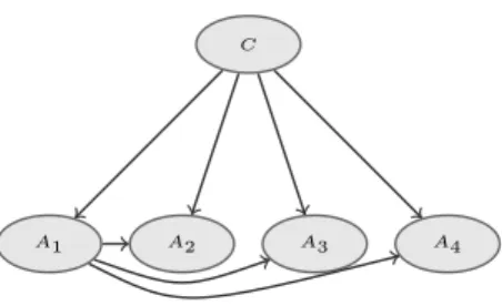
The AODE classifier [10] is based on a setS := {s1, . . . , sk}of kSPODEs (SuperParent-One-Dependence Estimator); in particular, SPODEsjhasAjas super-parent, namely it models all the remain-ing features as dependremain-ing on bothAjand on the classC, as shown in Figure 1.
Luc De Raedt et al. (Eds.) © 2012 The Author(s). This article is published online with Open Access by IOS Press and distributed under the terms of the Creative Commons Attribution Non-Commercial License. doi:10.3233/978-1-61499-098-7-264
C
A1 A2 A3 A4
Figure 1. SPODEs1with super-parentA1.
Such a topology induces in the joint probabilities of the SPODE
sjthe following factorization: P(c,a|sj) =P(c)·P(aj|c)·
l=1,...,k,l=j
P(al|aj, c). (1) To classify a test instance˜a, AODE simply averages the posterior probabilityP(c|˜a)computed by each SPODE. In this paper we study alternative approaches to aggregate the predictions of the SPODEs.
2.2
COMP-AODE: compression-based AODE
Compression-based averaging [1] overcomes the problem of BMA getting excessively concentrated around the single most probable model by replacing the posterior probabilities of the models with smoother,compressed, weights. We denote byη(sj|D) the weight assigned to modelsj.
We introduce anull classifier, denoted bys0, as a Bayesian net-work with no arcs, which models the class as independent from the features and whose probabilistic classifications correspond to the marginal probabilities of the classes. The null classifier is necessary to compute the compression coefficients.
Considering that all the SPODEs have the same number of vari-ables, the same number of arcs and the same maximum in-degree4, we assign the same prior probability to each SPODE. We instead as-sign prior probability=0.01 to the null model.Thus, we can consider a variableSwith values inS ∪ {s0}, and define the following prior mass function: P(sj) = j= 0, 1− k j= 1, . . . , k. (2) We compute theconditionallog-likelihood of SPODEsjas in [1]:
LLj:= n i=1
log(P(c(i)|a(i), sj,θˆj)), (3)
whereθjis a variable over the set of parameters for the model, and ˆ
θj is the value of its Bayesian estimation. It could be also possi-ble to evaluate the probability of the data given SPODEsj by the
marginallikelihood, i.e., P(D|sj) = P(D|sj, θj)P(θj|sj)dθj. Yet, the marginal likelihood measures how good the model is at rep-resenting thejointdistribution, while a classifier has instead to esti-mate the posterior probability of the classes byconditioningon the value of the features. Therefore, a model can poorly perform in clas-sification despite a high marginal likelihood [4]; the conditional like-lihood is a more appropriate score for classifiers.
4The in-degree is the number of parents of a node, and its maximum value is two for any SPODE.
IfLL0 is the conditional log-likelihood of the null model, then
LL0:=−nH(C), whereH(C) := −c∈CP(c) logP(c)is the
entropyof the class5[1]. The compression coefficients are computed in two steps: computation of therawcoefficients and normalization. Forj= 0, therawcompression coefficient of SPODEsjis defined as: ˜ ηj:= 1−loglogP(sj|D) P(s0|D) = 1− LLj+ log1−k −nH(C) + log. (4)
Ifη˜j is negative,sjis a worse predictor than the null model; if it is positive, as it normally happens,sjperforms better than the null model. The upper limit ofη˜jis 1, in which casesjis a perfect pre-dictor. Following [1], we keep in the ensemble thefeasiblemodels withη˜j>0, and we remove from the ensemble the remaining ones. This corresponds to removing from the ensemble the models whose posterior probability falls below a certain threshold, which is some-times done also when computing BMA. Since by definitionη˜0= 0, the null model is not part of the resulting ensemble.
Using the compression coefficients can be justified as follows [1]:
LLj+ logP(sj)“represents the quantity of information required to
encode the model plus the class values given the model. The code length of the null model can be interpreted as the quantity of infor-mation necessary to describe the classes, when no explanatory data is used to induce the model. Each model can potentially exploit the explanatory data to better compress the class conditional informa-tion. The ratio of the code length of a model to that of the null model stands for a relative gain in compression efficiency.”
Without loss of generality, we assume the features to be ordered, so that features {A1, A2, . . . , A˜k} yield a feasible model when used as super-parent; i.e., SPODEs{s1, s2, . . . , s˜k}are the feasi-ble ones. Thenormalizedcompression coefficients, which we denote asη(sj|D), are obtained by normalizing the raw compression coef-ficients of the feasible SPODEs:
η(sj|D) = η˜j ˜k l=1η˜l if j= 1, . . . , ˜ k, 0 otherwise. (5)
The posterior probabilities computed by COMP-AODE for instance ˜ aares: P(c|˜a) = k j=1 P(c|˜a, sj)·η(sj|D). (6)
2.3
Introducing a Set of Priors: COMP-AODE*
We extend COMP-AODE toimprecise probabilities[9], by allowing multiple specifications of the prior mass functionP(S); we denote byK(S) the so-calledcredal set of prior mass functions. A uni-form mass function represents priorindifferencebetween the differ-ent SPODEs; instead, a credal set provides a more cautious model of priorignoranceabout which SPODE might have produced the data.
In principle we could let the prior probabilities of each SPODE vary exactly between zero and one by considering any possible prior (vacuousmodel). Yet, this prevents learning from data, generating vacuous posterior inferences. To obtain non-vacuous posterior infer-ences, we introduce a non-zero lower bounds in the credal setK(S), which is defined as follows:
K(S) := ⎧ ⎨ ⎩P(S) P(s0) = P(sj)≥ j= 1, . . . , k k j=0P(sj) = 1 ⎫ ⎬ ⎭ (7)
5For this equivalence to hold, we compute the entropy using the natural log-arithm, instead of the log in basis 2.
The set in (7) is convex; itskextreme distributions are those assign-ing massto all the models apart from a single SPODE, which get mass1−k. WhenP(S)varies inK(S), therawcoefficients of compression, defined as in (4), span the following range:
ηj∈ 1− LLj+ log −nH(C) + log, 1− LLj+ log (1−k) −nH(C) + log . (8) However, the differentηjcannot vary in the intervals of Eq.(8) inde-pendently from each other, because of the normalization constraint of Eq. (7). Note moreover that since the prior of Eq.(2) is contained in the credal set, the point estimate of the compression coefficient used by COMP-AODE belongs to the interval.
We regard SPODEsjas non-feasible if theupperbound of the interval (8) is non-positive; this approach is particularly conservative as it preserves the models which are feasible (in the sense of Section 2.2) for at least a prior in the setK(X). COMP-AODE* is thus more conservative than COMP-AODE, namely it removes from the ensem-ble a lower number of models. However, in practice, no SPODE is generally removed from the ensemble neither by COMP-AODE*, nor by COMP-AODE.
Considering that K(S)is a set a prior mass functions, COMP-AODE* can be interpreted as a set of COMP-AODE classifiers, each induced in correspondence of a different prior. An instance is prior-dependentif the most probable class varies under the different priors of the credal set. COMP-AODE* remains reliable on prior-dependent instances, by returning a set of classes instead of a single one. Re-turning a set of classes on theprior-dependentinstances and a single class on the remainingsafeinstances is in fact the typical behavior of credal classifiers [3]. Note that prior-dependence is not a characteris-tic of the instance alone: a credal-classifier might judge an instance as prior-dependent, and an alternative credal classifier might judge it as safe. Thus, prior-dependence is a characteristic of a certain instance, when analyzed by aspecificcredal classifier.
2.3.1
Credal Dominance
Without loss of generality we assume the features reordered, so that the first˜kfeatures yield a feasible model, i.e., SPODEs{s1, . . . , s˜k} are the feasible ones. Given an unsupervised test instanceawhose class is unknown, classc∈ Cdominatesc∈ Cifcis more prob-able thancunder any prior of the credal set, i.e. if:
min P(S)∈K(S) P(c|a) P(c|a) = k˜ j=1P(c|a, sj)˜η(sj|D) k˜ i=1P(c|a, si)˜η(si|D) >1, (9) where, as we noted before, the sum over the feasible models corre-sponds to that over the firstk˜models and where we have substituted the standardized compression coefficients by the raw ones, having considered thatkj=1˜ η˜(sj|D)is positive by definition. The func-tion to be minimized in (9) then becomes:
˜k
j=1P(c|a, sj) (log−nH(C)−LLj−logP(sj))
˜k
i=1P(c|a, si) (log−nH(C)−LLi−logP(si))
.
By setting, for each j = 1, . . . ,˜k, xj := logP(sj), αj := P(c|a, sj),βj:=P(c|a, sj), and δ γ :=− ˜ k j=1 P(c|a, sj) P(c|a, sj) (log−nH(C)−LLj). (10)
the optimization problem to check whethercdominatescbecomes:
min x1,...,x˜k ˜k j=1αjxj+δ ˜k j=1βjxj+γ , subject to xj≥log j= 1, . . . ,˜k, k˜ j=1exj = 1−−(k−˜k).
The last constraint is related to the normalization constraint in the definition (7) of the credal set, and imposes the sum of the prior prob-ability of the feasible SPODEs to be one minus the prior probabilities of thek−˜knon-feasible SPODEs and the null model, whose prior probability is set to. We then substituteyj:=exj to avoid numeri-cal problems in the optimization, thus getting a non-linear optimiza-tion problem with linear constraints.
A class isnon-dominatedif no alternative class dominates it ac-cording to the test of Eq.(9). COMP-AODE* identifies the set of non-dominated classes through themaximalityapproach [9], which is commonly adopted for decision making with imprecise probabili-ties; for each instance it requires running the dominance test on each pair of classes, as formalized by Algorithm 1.
Since the credal set (7) includes the prior adopted by COMP-AODE, the non-dominated classes returned by COMP-AODE* in-clude by design the most probable class identified by COMP-AODE; thus, when COMP-AODE* returns a single class, it is the same class returned by COMP-AODE.
Algorithm 1 Identification of the non-dominated classes N D through maximality
N D:=C forc∈ Cdo
forc∈ C(c=c)do
compute the dominance test of Eq.(9) ifcdominatescthen removecfromN D end if end for end for return N D
2.4
Complexity
To analyze the computational complexity of the classifiers, we dis-tinguish between thelearningand theclassification complexity, the latter referring to the classification of a single instance. We analyze both thespaceand thetimerequired for computations. The orders of magnitude are reported as a function of the dataset sizen, the number of attributes/SPODEsk, the number of classesl:=|C|, and average number of states for the attributesv:=k−1ki=1|Ai|. A summary of this analysis is given in Table 1.
A single SPODEsjrequires storing the tablesP(C),P(Aj|C) andP(Ai|C, Aj), withi = 1, . . . , k andi = j, implying space complexityO(lkv2)for learning each SPODE andO(lk2v2)for the AODE ensemble. For each classifier, the same tables should be avail-able during learning and classification; thus, space requirements of these two stages are the same. Time complexity to scan the dataset and learn the probabilities is O(nk) for each SPODE, and hence
O(nk2) for the AODE. The time required to compute the poste-rior probabilities as in Eq.(1) isO(lk)for each SPODE, and hence
Algorithm Space Time
learning/classification learning classification
AODE O(lk2v2) O(nk2) O(lk2)
COMP-AODE O(lk2v2) O(n(l+k)k) O(lk2) COMP-AODE* O(lk2v2) O(n(l+k)k) O(l2k3)
Table 1. Complexity of classifiers.
O(lk2)for AODE. Learning COMP-AODE takes roughly the same space as AODE, but higher computational time, due to the evaluation of the conditional likelihood of Eq.(3). The additional computational time isO(nlk), thus requiringO(n(l+k)k)time overall. For clas-sification, time and space complexity is equivalent to that of AODE. COMP-AODE* has the same space complexity of COMP-AODE and the same time complexity in learning, but higher time complex-ity in classification. The pairwise dominance tests in Algorithm 1 require solving a number of optimization problems for each test in-stance which is quadratic in the number of classes. Each optimiza-tion has time complexity which is roughly cubic in the number of constraints/variables, which is in turnO(k).
Compared to AODE, the new classifiers require higher training time, while the higher cautiousness characterizing COMP-AODE* increases by one the exponents of the number of classes and attributes in the complexity of the classification time.
3
Experiments
We run experiments on 40 UCI data sets, taken from the UCI reposi-tory; the sample size ranges between 57 (labor) and 12960 (nursery); the number of classes between 2 and 10 (pendigits). On each data set we perform 10 runs of 5-folds cross-validation. Missing data are replaced by the median/mode for numerical/categorical features, so that all data sets are complete. We discretize numerical features by the MDL-based discretization [6]. For AODE, we set to 1 the fre-quency limit; namely, features with a frefre-quency in the training set below this value are not used as parents; this is also the default value in WEKA.
In order to compare two classifiers over the collection of data sets we use the non-parametric Wilcoxon signed-rank test.6This test is indeed recommended for comparing two classifiers on multiple data sets [5]: being non-parametric it both avoids strong assumptions and deals robustly with outliers.
3.1
AODE vs. COMP-AODE
We consider two indicators: the accuracy, namely the percentage of correct classifications, and the Brier loss:
1 nte
nte i
1−P(c(i)|a(i))2 where n
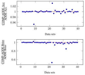
te denotes the number of instances in the test set and P(c(i)|a(i)) is the probability estimated by the classifier for the true class of thei-th instance of the test set. In Figure 2(a) we show therelative accuracies, namely the accuracy of COMP-AODE divided, separately for each data set, by the accuracy of AODE. Thus, better performance relatively to AODE is achieved when the relative accuracy is>1. The accuracy of the two models is identical (relative accuracy = 1) in 15/40 cases ; in 14/40 data sets relative accuracy is>1 (COMP-AODE wins) while 6We use the test as follows: for a given indicator we build twopairedvectors, one for each classifier: the same position refers, in both vectors, to the same data set. The two vectors are then used as input for the test.
in 11/40 data sets relative accuracy is<1 (AODE wins). Overall, the performance of COMP-AODE and AODE on this collection of data sets is not significantly different. In Fig.2(b), we show therelative Brier losses, namely the Brier loss of COMP-AODE divided, data set by data set, by the Brier loss of AODE; thus, better performance relatively to AODE is achieved when the relative Brier loss is <1. The Brier loss is more sensitive than accuracy, and thus magnifies the differences among classifiers, as can be seen by comparing the scales of relative accuracies and relative Brier losses. Under Brier loss, COMP-AODE performs significantly better than AODE (p-value<0.01). The Brier loss of the two models is identical (relative loss = 1) in 12/40 cases ; in 23/40 data sets relative loss is
<1 (COMP-AODE wins) while only in 5/40 data sets relative loss is
>1 (AODE wins). This is noteworthy given the high performance of AODE and the fact the standard AODE often outperforms alternative weighting methods over SPODEs [11]. Our findings thus extend the results of [1] in which the compression-based approach was successfully applied over an ensemble of naive Bayes classifiers.
0 10 20 30 40 0.96 0.98 1 1.02 Data sets COMP-A ODE Acc A ODE Acc 0 10 20 30 40 0.6 0.8 1 Data sets COMP-A ODE Brier A ODE Brier
Figure 2. Relative accuracies and relative Brier losses: for accuracy, performance better than AODE corresponds to points lyingabovethe horizontal line; for Brier loss, performance better than AODE corresponds to
points lyingbelowthe horizontal line. Note the different scale of the two graphs, reflecting the higher sensitivity of Brier loss.
3.2
Evaluation of COMP-AODE*
A credal classifier separates in fact the instances into two groups: thesafeones, for which a single class is returned, and the prior-dependentones, for which instead different non-dominated classes are returned. To fully characterize the performance of an impre-cise classifier, four indicators can be considered:determinacy: the proportion of instances recognized as safe and thus classified with a single class;single-accuracy: the accuracy achieved over the in-stances recognized as safe;set-accuracy: the accuracy achieved over the prior-dependent instances, by returning a set of classes; indeter-minate output size: the average number of classes returned on the prior-dependent instances.
COMP-AODE* is generally very determinate: its average deter-minacy is 99%; this means that on average it recognizes only 1% of the instances as prior-dependent. This is probably a consequence of
the logarithmic smoothing induced by the compression coefficients, which makes the weights of the models little sensitive on the chosen prior. We see this robustness to the choice of the prior as a desir-able and previously unknown property of the compression-based ap-proach; in fact, it is easy investigating this point only once developed the credal classifier. The robustness to the choice of the prior might well constitute a further reason for the good empirical performance of the compression-based approach. COMP-AODE* performs well when indeterminate: averaging over all data sets, it achieves 95% set-accuracy by returning 2 classes. In Fig.3, we compare the ac-curacy achieved by COMP-AODE on the instances judged respec-tively safe and prior-dependent by COMP-AODE*. Each point refers to a different data set; for that data set, it represents the accuracy achieved by COMP-AODE on the safe instances (y-coordinate) and on the instances judged as prior-dependent by COMP-AODE* (x -coordinate). On almost every data set, the accuracy of COMP-AODE is much higher on the safe instances than on the prior-dependent instances (y x) ; the drop of accuracy between the safe and the prior-dependent instances is indeed significant (p-value<0.01). As a rough indication, averaging over data sets, the accuracy of COMP-AODE is 82% on the safe instances but only 47% on the prior-dependent instances. Thus, while COMP-AODE provides frag-ile classifications on the prior-dependent instances, COMP-AODE* remains reliable by returning a small-sized but highly reliable set of classes. Thus even COMP-AODE, despite its robustness to the spec-ification of the prior, undergoes a severe loss of accuracy on the in-stances recognized as prior-dependent by COMP-AODE*; on these instances, as already discussed, COMP-AODE* preserves its relia-bility thanks to indeterminate classifications.
0 0.2 0.4 0.6 0.8 1 0 0.5 1 prior-dependentinstances safe instances Accuracy COMP-AODE
Figure 3. Accuracy of COMP-AODE on the instances recognized as safe and as prior-dependent by COMP-AODE*; the straight line is thebisectrix.
3.3
Utility-based Measures
We have seen that AODE* extends in a sensible way COMP-AODE, being able to recognize prior-dependent instances and to robustly deal with them. To further compare COMP-AODE and COMP-AODE*, we adopt the utility-based measures of [12]. In fact, how to compare determinate and indeterminate predictions is far from obvious. Thediscounted accuracyrewards a prediction made of m classes with1/m if it contains the actual class, and 0 oth-erwise; the discounted accuracy of a credal classifier can be then compared to the accuracy of a determinate classifier. However [12] points out some severe limits of discounted-accuracy, which we il-lustrate by means of an example. We consider two medical doc-tors,randomand doctorvacuous, whose task is to classify each pa-tient in one of the two categories{healthy, diseased}. Doctor
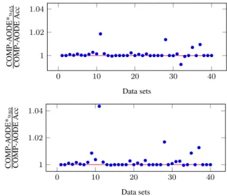
ran-0 10 20 30 40 1 1.02 1.04 Data sets COMP-A ODE* u65 COMP-A ODE Acc 0 10 20 30 40 1 1.02 1.04 Data sets COMP-A ODE* u80 COMP-A ODE Acc
Figure 4. Relative utilities; a better performance of COMP-AODE* over COMP-AODE is represented by points lyingabovethe horizontal line.
dom generates random diagnoses, drawing its judgment from a uni-form probability mass function. Doctor vacuous instead always re-turns both categories, admitting to be ignorant. Let us assume that the hospital receives a quantity of money which is proportional to the discounted-accuracy generated by its doctors when visiting pa-tients. Both doctors provide the sameexpecteddiscounted-accuracy (1/2) and thus the sameexpectedprofit; yet, the profit generated by doctor vacuous is deterministic, while the profit generated by doctor random is affected by considerable variance. Under any risk-averse utility function, doctor vacuous generates a higherutilitythan doctor random, yielding the same expected reward but with less variance: under risk-aversion, the expected utility increases with expectation of the rewards and decreases with their variance (see the references in [8]). In [12] it is thus proposed to compare credal and determi-nate classifiers measuring the utilityof the reward constituted by discounted-accuracy: the stronger the risk aversion, the higher the value of indeterminate but accurate (containing the true class in the set of non-dominated classes) predictions. In [12] the utility of a cor-rect and determinate classification (discounted-accuracy 1) is set to 1; the utility of a wrong classification (discounted-accuracy 0) to 0; the utility of an accurate but indeterminate classification consisting of two classes (discounted-accuracy 0.5) is assumed to lie between 0.65 and 0.8, depending on the degree of aversion. In correspondence of these two values, two quadratic utility functions are derived:u65 passes through{u(0) = 0, u(0.5) = 0.65, u(1) = 1}, whileu80 passes through{u(0) = 0, u(0.5) = 0.8, u(1) = 1}. In real appli-cations the utility function should be elicited by discussion with the decision maker; in this paper we useu65andu80to model two rea-sonable but different degrees of risk-aversion. Sinceu(1) = 1, the utility and the accuracy of a traditional classifier coincide; therefore the utility values of credal classifiers can be directly compared with the predictive accuracy of the traditional classifiers. In [7] classifiers which return indeterminate classifications are scored through theF1 -metric, originally designed for Information Retrieval tasks. TheF1 metric, when applied to indeterminate classifications, returns a score which is always comprised betweenu65andu80, further confirming the reasonableness of these utility functions.
di-vided, data set by data set, by the accuracy of COMP-AODE. The two plots refer respectively to u65 andu80. Some points are ex-actly 1, since in some data sets COMP-AODE is completely determi-nate. However, the points tend to be generally higher than 1; COMP-AODE* generates significantly higher utility (p-value<0.01) than COMP-AODE under bothu65andu80. The numerical improvement is generally small, being close to 1%; however this is reasonable if we consider that COMP-AODE* has 99% determinacy on average. The improvement of COMP-AODE* over COMP-AODE is more evident underu80, due to the higher utility associated in this case to classi-fications which are accurate but indeterminate. Moreover, COMP-AODE* generates significantly (p-value <.01) higher utility than AODE, underbothu65andu80. The extension to imprecise proba-bility has thus improved performance of the compression-based en-semble: recall that the determinate COMP-AODE yields better prob-ability estimates but not better accuracy than AODE.
3.4
Comparison with Other Credal Classifiers
Previous credal classifiers, which return more classes on the in-stances identified as prior-dependent, include for instance thenaive credal classifier(NCC), namely an extension of naive Bayes to im-precise probability and thecredal model averaging(CMA), a gen-eralization of BMA over naive Bayes classifiers, in the same spirit of Section 2.3 but without compression. We point the reader to [3] for more insights and references on previous credal classifiers. Here we compare the performances of NCC, CMA and COMP-AODE* by means of the utility measures u65 andu80, adopting the same experimental setup detailed at the begin of Section 3. We compare these classifiers over the collection of 40 data sets by the Friedman test coupled with the Nemenji post-hoc, as recommended in [5]. Un-der bothu65andu80we thus eventually rank the credal classifiers according to the utility they generate. Figure 5 reports the results of this comparison for bothu65andu80. The post-hoc analysis, un-deru65, ranks COMP-AODE* as significantly better than both CMA and NCC. Underu80no significant difference is found among clas-sifiers; the point is that both CMA and NCC are much more indeter-minate than COMP-AODE*, and benefit at a much larger extent than COMP-AODE* from the increase utility assigned byu80to indeter-minate but accurate classifications; in this way, they close the gap with COMP-AODE*. However, also underu80COMP-AODE* has the highest average rank, and we conclude that COMP-AODE* pro-vides a generally higher classification performance than both CMA and NCC.
4
Conclusions
COMP-AODE is a new classifier based on compression-based av-eraging of SPODEs; it slightly but significantly improves classifica-tion performance over AODE. COMP-AODE* extends it to impre-cise probability, by replacing the single uniform prior over SPODEs with a credal set of priors. COMP-AODE* returns more classes on the instances recognized as prior-dependent and achieves higher pre-diction utility than both COMP-AODE and AODE.
Acknowledgments
Research partially supported by Swiss NSF grant no. 200020-132252 and the Hasler foundation grant n. 10030.
1 2 3 4 COMP-AODE* CMA NCC Ranks underu65 1 2 3 4 COMP-AODE* CMA NCC Ranks underu80
Figure 5. Comparison between credal classifiers. The points denote the average ranks, while the bars display the critical distance. The average ranks
of two classifiers are significantly different if they differ by more than the critical distance, namely if their bars do not overlap.
References
[1] M. Boull´e, ‘Compression-based averaging of selective naive Bayes classifiers’, Journal of Machine Learning Research,8, 1659–1685, (2007).
[2] J. Cerquides, R.L. De M`antaras, et al., ‘Robust Bayesian linear classi-fier ensembles’,Lecture notes in computer science,3720, 72, (2005). [3] G. Corani, A. Antonucci, and M. Zaffalon, ‘Bayesian networks with
im-precise probabilities: Theory and application to classification’, inData Mining: Foundations and Intelligent Paradigms, eds., D. E. Holmes, L. C. Jain, and J. Kacprzyk, volume 23, 49–93, Springer, (2012). [4] R. Cowell, ‘On searching for optimal classifiers among Bayesian
net-works’, inProceedings of the Eighth International Conference on Arti-ficial Intelligence and Statistics, pp. 175–180, (2001).
[5] J. Demsar, ‘Statistical comparisons of classifiers over multiple data sets’,Journal of Machine Learning Research,7, 1–30, (2006). [6] U. M. Fayyad and K. B. Irani, ‘Multi-interval discretization of
continuous-valued attributes for classification learning’, inProc. 13th Int. Joint conference on artificial intelligence (IJCAI-93), pp. 1022– 1027, (1993).
[7] J. Jose del Coz and A. Bahamonde, ‘Learning nondeterministic classi-fiers’,Journal of Machine Learning Research,10, 2273–2293, (2009). [8] H. Levy and H.M. Markowitz, ‘Approximating expected utility by a function of mean and variance’,The American Economic Review, 69(3), 308–317, (1979).
[9] P. Walley,Statistical Reasoning with Imprecise Probabilities, Chapman and Hall, New York, 1991.
[10] G.I. Webb, J.R. Boughton, and Z. Wang, ‘Not so naive Bayes: Ag-gregating one-dependence estimators’,Machine Learning,58(1), 5–24, (2005).
[11] Y. Yang, G.I. Webb, J. Cerquides, K.B. Korb, J. Boughton, and K.M. Ting, ‘To select or to weigh: A comparative study of linear combination schemes for superparent-one-dependence estimators’,Knowledge and Data Engineering, IEEE Transactions on,19(12), 1652–1665, (2007). [12] M. Zaffalon, Corani G., and D. Mau´a, ‘Utility-based accuracy measures
to empirically evaluate credal classifiers’, inISIPTA’11: Proceedings of the Seventh International Symposium on Imprecise Probability: Theo-ries and Applications, pp. 401–410, (2011).