OFM-ERDC-WDQI-Post Secondary Earnings Premium Study 2014 Page 1 Earnings Premium Estimates for Bachelor’s Degrees in Washington State
Toby Paterson
Education Research and Data Center Workforce Data Quality Initiative Project
Greg Weeks, Ph.D.
Education Research and Data Center Workforce Data Quality Initiative Project
Washington State
Office of Financial Management 210 11th AVE SW, Room 318
PO BOX 43113 Olympia, WA 98504-3113
OFM-ERDC-WDQI-Post Secondary Earnings Premium Study 2014 Page 2
Table of Contents
Abstract ... 4
Acknowledgments ... 4
Executive Summary ... 5
Executive Summary Chart. College earnings premium in 2012 dollars, follow up years 1-7. ... 6
Figure 1. Expected patterns of earnings for high school and bachelor’s degree graduates. ... 9
2. Previous Research ... 9
3. Analytical Approach ... 11
3.1. Propensity Score ... 124. Data ... 13
5. Estimation Methodology ... 14
Figure 2. Follow up years after high school graduation. ... 14
6. Findings ... 15
Chart 1. College earnings premium in 2012 dollars, follow up years 1-7. ... 15
Chart 2. College earnings premium as a percent of HS only group, follow up years 1-7. ... 16
Chart 3. Female college earnings premium, 2012 dollars, follow up years 1-7. ... 16
Chart 4. Male college earnings premium, 2012 dollars, follow up years 1-7. ... 17
Chart 5. Female and male college earnings premium, 2012 dollars, follow up years 1-7. ... 18
7. Conclusion ... 18
Chart 6. Female to male earnings differential, 2012 dollars, follow up years 1-7. .. 19
Chart 7. Female to male earnings percent differential, 2012 dollars, follow up years 1-7. ... 20
References ... 21
Appendix A: Matching ... 22
Appendix B: Enrollment Data Sources & Definitions... 23
Appendix C: Unemployment Insurance ... 24
Figure C-1: Timing of collection and availability of UI wage data. ... 25
Appendix D: Data flow, merging and edits ... 26
OFM-ERDC-WDQI-Post Secondary Earnings Premium Study 2014 Page 3
Figure D2. This figure shows the sample size by calendar year for each cohort and group. ... 26
Appendix E. Average annual cost of tuition and fees and books and supplies. .. 27
Table E1. Average annual cost of tuition and fees and books and supplies,
OFM-ERDC-WDQI-Post Secondary Earnings Premium Study 2014 Page 4 Abstract
This paper examines the earnings of workers with bachelor’s degrees from Washington state public colleges and universities compared to the earnings of workers with public high school diplomas only. We use propensity score matching to control for selection bias. Our analysis is based on data from the Washington State Education Research and Data Center (ERDC). We find earnings gains associated with obtaining a bachelor’s degree to be 19 percent for females and 18 percent for males seven years after graduation.
JEL Classification: C23, H40, I21, J24, J31
Keywords: propensity score matching, selection bias, returns to education, college earnings premiums
Acknowledgments
We thank Gary Benson, George Hough, Carol Jenner, Marieka Klawitter and Ernst Stromsdorfer, for their detailed review, insights and helpful comments. The authors retain responsibility for any remaining errors. The views expressed in this paper are those of the authors and not necessarily those of the Office of Financial Management, the Education Research and Data Center, or the Department of Labor. We acknowledge the financial support of the United States Department of Labor through the Work Force Data Quality Initiative grant.
OFM-ERDC-WDQI-Post Secondary Earnings Premium Study 2014 Page 5 Executive Summary
As the United States emerges from the recession of 2007-2009, post-secondary education becomes important both as a strategy for macroeconomic growth and as a means for individuals to increase their lifetime earnings. Both goals depend upon post-secondary
education leading to increased human capital, productivity and earnings. This paper estimates the earnings premium associated with a bachelor’s degree in the state of Washington, adjusting for selection bias.
The Education Research and Data Center in the Office of Financial Management is developing and implementing a longitudinal education data warehouse for Washington state, funded by the US Department of Education. The current study is funded by the Washington state Workforce Data Quality Initiative grant to promote the value of connecting education with workforce information.
We utilize a propensity score matching (PSM) approach to minimize the effects of selection bias in this study. The propensity score is the estimated probability that a high school graduate will earn a bachelor’s degree within five years. This approach matches treatment group members who have bachelor’s degrees to individual comparison group members who have high school diplomas only based on their respective propensity scores. The resulting treatment and comparison groups are closely matched on the observed characteristics important to the college graduation outcome.
This is a cohort study, with the cohorts defined by year of high school graduation. All three cohorts (2005, 2006 and 2007 high school graduates) in this study graduated from high school just prior to the recession of 2007-2009. Females and males are modeled separately. We assess the impact on earnings of obtaining a bachelor’s degree by comparing median earnings by year since high school graduation. For each cohort we calculate inflation adjusted earnings for each calendar year covered by the study.
The principal results of this research are summarized in the executive summary chart. This chart shows the bachelor’s degree earnings premium expressed as the difference between the Bachelor’s degree group earnings and the HS only group earnings. Generally, for both genders, we find substantial forgone earnings (opportunity cost) associated with college attendance, ranging up to $14,000 per year for males and up to $9,800 per year for females. On the other hand, after year four for females and year five for males, the earnings premium for college turns positive, and increases thereafter for every year covered by the follow up data.
By year seven, female bachelor’s degree earners have median earnings that are $5,400 above the median for HS only females, a 19 percent college earnings premium. The male bachelor’s degree earners have opened an even larger earnings premium above HS only workers: earning $6,200 more when median earnings are compared, an 18 percent college earnings premium.
OFM-ERDC-WDQI-Post Secondary Earnings Premium Study 2014 Page 6 Executive Summary Chart. College earnings premium in 2012 dollars, follow up years 1-7. Throughout the follow up period the female to male earnings differential is consistently negative (women earn less). For the high school group, females consistently earn between $4,500 and $7,200 less per year than male HS only workers. For the Bachelor’s degree group, through the first four years of follow up, females and males earn roughly the same amounts per year, ranging from women having a $1,200 deficit in year one to only a $100 deficit in year four. After attainment of the bachelor’s degree, the relative earnings of female workers fall relative to male workers. By follow up year seven, females earn $6,100 less than males with bachelor’s degrees. This amounts to an 18 percent differential, the same as the follow up year seven differential for the HS only group.
-$6,888 -$8,358 -$9,838 -$6,208 $358 $4,775 $5,432 -$10,103 -$13,948 -$13,963 -$13,330 -$3,906 $1,516 $6,226 -$15,000 -$10,000 -$5,000 $0 $5,000 $10,000 1 2 3 4 5 6 7 Dollars Follow up years
Bachelor’s degree earnings premium and opportunity cost (negative values) for follow up years 1-7 after HS graduation, females and males, 2012 dollars
OFM-ERDC-WDQI-Post Secondary Earnings Premium Study 2014 Page 7 1. Introduction
As the United States emerges from the recession of 2007-2009, post-secondary education becomes important both as a strategy for macroeconomic growth and as a means for individuals to increase their lifetime earnings. Both goals depend upon post-secondary
education leading to increased human capital, productivity and earnings. This paper estimates the earnings premium associated with a bachelor’s degree in the state of Washington, adjusting for selection bias.
While the earnings premium for post-secondary education has increased in recent years, this has not always been the case. In the US, the earnings premium for post-secondary education “decreased in the 1940s, rose in the 1950s and 1960s, fell in the 1970s, and since that time has increased substantially” (Goldin and Katz 2008, p. 71). Goldin and Katz find that the recent and dramatic increase in returns to education is due both to changes in the demand for educated workers (skill-based technological change) and changes in the supply of educated workers. “The slowdown in the growth of educational attainment… is the single most important factor increasing educational wage differentials since 1980 and is a major contributor to increased family income inequality” (ibid. p. 325). These issues are difficult to analyze empirically. Fortunately, in many states, there is a new source of educational data that is well suited to address these issues.
Many states are developing and implementing longitudinal education data warehouses under the State Longitudinal Data Systems (SLDS) grants issued by the US Department of Education. These data warehouses provide researchers with the capability to access unit record data about students’ academic progress from pre-kindergarten through graduate school. With near
universal micro-level data, these systems provide the opportunity for unparalleled levels of accountability, analysis and research. The US Department of Labor has funded a series of state Workforce Data Quality Initiative (WDQI) grants to promote the inclusion of Unemployment Insurance (UI) earnings and employment data in these data warehouses.
This educational study is funded by the Washington state WDQI grant administered by the Education Research and Data Center (ERDC) in the Office of Financial Management. The study demonstrates the value of connecting micro-level education data with micro-level workforce data. This study is the first in a series which will provide information on the economic returns to post-secondary education in Washington state. This study examines the economic (earnings) impacts of the attainment of a bachelor’s degree from a public four year college or university in Washington state compared to students who completed their high school (HS only) diploma, but had no post-secondary education of any kind.
Throughout this study we use the terms “Bachelor’s degree” to refer to the treatment group and “HS only” to refer to the comparison group. This assessment is challenging because the determinants of earnings include more than educational attainment. Many factors influence both the decision to attend college and subsequent earnings, which will confound the findings
OFM-ERDC-WDQI-Post Secondary Earnings Premium Study 2014 Page 8 unless taken into account. These factors include: academic ability, work effort and persistence, future versus present orientation, parents’ income and education and the students’ propensity to attend and graduate from college. These factors are often collectively summarized as to contributing to selection bias. Simply measuring the post-graduation earnings of college graduates and comparing them to the earnings of high school graduates will overstate the returns to college because the college graduates would have higher earnings even in the absence of college attendance, given the effects of the above background characteristics. Selection bias is not a factor in random assignment based experimental studies because the treatment and comparison groups are statistically identical. Unfortunately, such an approach is generally unavailable for educational research. Like other educational research, this is an observational study based on administrative data. The treatment and comparison groups upon which this study is based are Washington state high school graduates from 2005-2007. Each year’s graduating class defines a cohort for the study. The data are from the ERDC.
Throughout the literature covering the post-secondary earnings premium, outcomes are commonly overstated due to uncontrolled selection bias. Caponi and Plesca (2007) mention the sparseness of research on post-secondary returns and the persistent problem of ignored selection bias. They give estimates of the selection corrected percent earnings premium:
“However, the literature does not account for the possibility that the estimated returns to education suffer from the selection bias that arises when the choice of education is related to unobserved characteristics, for example innate ability, which also affect earnings... Once ability selection is accounted for by our propensity score matching procedure, the university returns relative to high-school decrease from 0.45 to 0.35 for males and from 0.45 to 0.41 for females” (Caponi and Plesca, 2007, p. 1).
We utilize a propensity score matching (PSM) technique to minimize the effects of selection bias in this study. “The propensity score is the conditional probability of assignment to a particular treatment given a vector of observed covariates” (Rosenbaum and Rubin, 1983, p. 41). This approach matches Bachelor’s degree group members to HS only group members based on their respective propensity scores. The resulting Bachelor’s degree and HS only groups are closely matched on the observed characteristics important to college graduation outcomes.
While it is not possible to know that selection bias has been eliminated from any observational study, the PSM technique represents the best available method and is prevalent in the
evaluation literature. “Approaches that directly match participants with nonparticipants who have similar (observed) characteristics have replaced regression as one of the preferred methods for estimating intervention impacts using comparison group data” (Heinrich, Maffioli and Vezquez 2012, p. 4). (Parentheses added.) This approach is discussed in more detail in section three below.
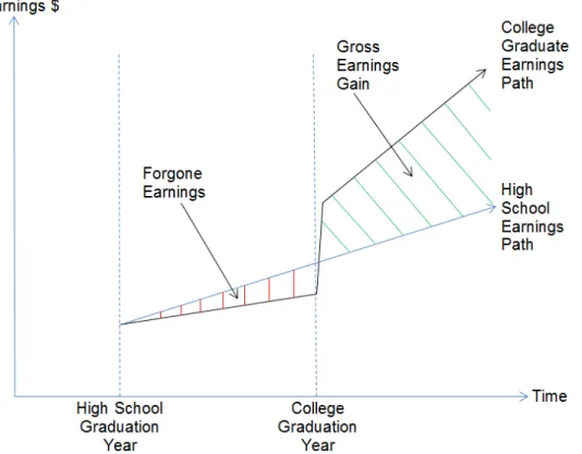
Figure 1 shows the expected patterns of earnings for the two study groups after high school graduation. Initially, through about year five after high school, the college degree earners are
OFM-ERDC-WDQI-Post Secondary Earnings Premium Study 2014 Page 9 expected to earn less than the matched high school only comparison group. These forgone earnings represent the opportunity cost of attending college. After year five, the earnings of the college degree earners should increase relative to HS only, reflecting the increased human capital, productivity and earnings potential associated with a college degree.
Figure 1. Expected patterns of earnings for high school and bachelor’s degree graduates. The core hypothesis of this study is represented in Figure 1 by the green crosshatched area labeled “Gross Earnings Gain,” and can be stated as: “The earnings of college graduates exceed the earnings they would have achieved if they had no post-secondary education.”
This paper is organized as follows. Section 2 describes previous research assessing the earnings gains associated with a bachelor’s degree. Section 3 discusses the paper’s analytical approach, including our use of propensity score estimation and matching. Section 4 describes the data used in this study. Section 5 describes our estimation methodology. Section 6 discusses our findings. We complete the paper with conclusions and observations.
2. Previous Research
There are a number of educational research studies which directly compare average earnings between groups with different levels of educational attainment. While these studies often claim to show a college earnings premium, they actually show an earnings premium that is
OFM-ERDC-WDQI-Post Secondary Earnings Premium Study 2014 Page 10 partly attributable to the differences in characteristics between graduates and non-graduates (selection bias), and differences partly attributable to the attained education level. Such studies commonly do not distinguish between these two aspects of the earnings premium, and thereby overstate the returns to educational attainment.
A recent prominent study entitled “Higher Education Pays: But a Lot More for Some Graduates Than for Others” compares average earnings for bachelor’s degrees by major with a variety of other post-secondary degrees and certificates (Schneider, 2013). The data upon which the paper is based reflect an impressive effort to utilize the education and earnings data from five states: Arkansas, Colorado, Tennessee, Texas and Virginia. These states provided detailed post-secondary educational attainment data matched to earnings information for the first year after graduation. A key finding from the paper is that the average earnings for some technical associate’s degree programs exceed the average earnings of bachelor’s degree holders. Unfortunately, because the study ignores selection bias, this differential cannot be
disaggregated into the portion attributable to student characteristics and the portion resulting from the intrinsic human capital value of the attained degree. It leaves unexplored the degree to which the earnings differentials described in the paper estimate the economic value of the obtained degrees rather than differences in the characteristics and backgrounds of the students.
A second study by Baum, Ma, and Payea (2013) uses a similar approach. The authors measure the annual median earnings by educational attainment. While the authors do not adjust for selection bias, or any differences between groups with different levels of education, they do offer information on a wide variety of outcomes. These outcomes range from demographic characteristics to civic involvement. This range of topics demonstrates the broad reach of education to outcomes beyond earnings. Their study also fails to account for selection bias and also is likely to overstate the earnings premium for post-secondary education throughout the analysis. However, because earnings are not normally distributed the median is a better measure of central tendency and moderates the impacts of extreme values.
There have also been a number of studies on the returns to education with a more macro-economic perspective. Focusing on education and skill-based technological change, these studies compare the aggregate earnings of degree holders relative to non-degree holders over time. To the extent that the selection factors are time invariant, the effects of selection may cancel when comparing one time period with another. Goldin and Katz (2008) may be the best example of analyzing the connection between education and skill based technological change. Their work has led to numerous articles and studies on the macroeconomic educational
earnings premium. A recent example focuses on the effects of college major (James, 2013). However, James does not compare one time period with another, so that the selection bias factors are present. He ignores selection bias and his findings may be overstated.
There have been few recent studies of the returns to post-secondary baccalaureate education that correct for selection bias. Among the most comprehensive is a study by Caponi and Plesca (2009). They use data from the Canadian General Social Survey to estimate the returns to both
OFM-ERDC-WDQI-Post Secondary Earnings Premium Study 2014 Page 11 college (community college) and university (baccalaureate) educational attainment. They “test” three approaches to selection bias: OLS regression, the classical Heckman two-step selection adjustment, and a propensity score matching approach. They conclude that “Among the estimators implemented to correct for selection bias we find propensity score matching to be the most reliable one, given identification assumptions and available data” (p. 1124). They found average treatment effects of 34 percent higher earnings for males and 39 percent higher earnings for females. They also simulated the internal rates of return for males and females separately. Using the PSM technique they estimated an internal rate of return of 13 percent for females, and 10 percent for males.
Wen Fan (2011) conducted a propensity score matching analysis of British students who were eligible for admission into university. He used the British Cohort Study (1970) data, which provided a rich set of explanatory variables for the propensity score estimates. He compared two matching methods, nearest neighbor matching, and a kernel matching algorithm. He found average treatment effects of 41 percent higher earnings with nearest neighbor matching and 51 percent higher earnings with Kernel matching for college eligible students. He did not estimate males and females separately.
3. Analytical Approach
There is an extensive literature on the topic of correcting selection bias in observational studies. Smith and Todd (2005) refer to articles by Heckman, Ichimura and Todd (1997) and Heckman, Ichimura, Smith and Todd (1998) in which the latter authors use non-experimental propensity score techniques to estimate net economic effects from an experimentally designed evaluation study as a way to evaluate the propensity score matching approach. Referring to these
authors, Smith and Todd state that:
“…data quality is a crucial ingredient to any reliable estimation strategy. Specifically, the
estimators examined are only found to perform well in replicating the results of the experiment when they are applied to comparison group data satisfying the following criteria: (i) the same data sources (i.e., the same surveys or the same type of administrative data or both) are used for participants and nonparticipants, so that earnings and other characteristics are measured in an analogous way, (ii) participants and nonparticipants reside in the same local labor markets, and (iii) the data contain a rich set of variables that affect both program participation and labor market outcomes” (p. 309).
The Washington Education Research and Data Center data fully meet these requirements. We apply a propensity score matching technique to develop a comparison group to serve as the counterfactual to the treatment group. We use logistic regression to estimate propensity scores for the combined Bachelor’s degree and HS only groups. The propensity score acts as a single number index of the variables that are used in its estimation.
We institute a one-to-many with replacement matching algorithm, where HS only group members are matched to one or more Bachelor’s degree group members. We recognize this
OFM-ERDC-WDQI-Post Secondary Earnings Premium Study 2014 Page 12 technique increases the level of precision at the cost of increasing bias (Dehejia and Wahba, 2007, pp. 151-158). See Appendix A for a discussion of these issues.
The primary advantage the present study has over previous studies is our access to data from cohorts of high school students who did not experience any post-secondary education. This is an ideal comparison pool for an observational study using PSM methods. Treatment and comparison group members should have the same distributions of observed and unobserved attributes and come from similar economic environments to effectively reduce the selection bias (Heckman, Ichimura, Todd, 1997, p. 606). To a considerable extent, the HS only group had the same primary and secondary educational experiences and opportunities as the Bachelor’s degree group. Also, both groups were raised in the same neighborhoods, and had access to the same labor markets during and after high school. These similarities reduce the differences between the two groups and enhance the likelihood that the PSM technique corrects for selection bias.
3.1. Propensity Score
The propensity score method reduces the dimensionality of the selection characteristics of sample members. Each cohort member is assigned an estimated propensity score value. Females and males are modeled separately, while the bachelor’s degree earners (treatment) and the high school only (comparison) groups are modeled together for each gender and cohort. The calculation uses a logistic regression technique. The model specification that we use was selected by testing alternative model specifications and evaluating the statistical properties of each specification. The independent variables that make up the characteristics vector of the selected model are: high school grade point average (GPA), free and reduced price lunch eligibility (FRPL), county and county unemployment rate. The binary dependent variable is the treatment, obtaining a bachelor’s degree.
P(T) = α + β1(GPA) + β2(FRPL) + β3(County) + β4(Unemployment rate) + ε
Where P(T) is the probability of obtaining a bachelor’s degree for any student, α is the intercept, the β’srepresent the parameter coefficient estimates, GPA is the student’s grade point average, county represents the county of the student’s high school, unemployment rate is the student’s high school county unemployment rate, and ε is the residual error term.
The propensity scores representing the probability of obtaining a bachelor’s degree within five years are used to directly match individuals in the HS only group to individuals in the Bachelor’s degree group. The matching process minimizes the total distance between propensity scores for the two groups. Matching is done with replacement (see Appendix A).
OFM-ERDC-WDQI-Post Secondary Earnings Premium Study 2014 Page 13 4. Data
We start with the roster of graduates from public high schools in Washington State, extracted from the annual ERDC High School Feedback Reports (ERDC, 2013). High school graduates from each of the cohort years comprise the study population. Students who graduated from a Washington state public high school in 2005 comprise cohort one. The 2005 high school
graduates who earn a bachelor’s degree from a public university in Washington state within five years of high school graduation (spring 2010) comprise the cohort one Bachelor’s degree group (the five year graduation criteria is applied to all the cohorts). The 2005 high school graduates with no post-secondary education experience whatsoever make up the cohort one HS only group.
Based on information from the ERDC and the National Student Clearinghouse (NSC), Bachelor’s degree group members who were attending an out-of-state college or university or attending an in-state private college or university are eliminated from the study population. Also, Bachelor’s degree group members who were enrolled in post-baccalaureate studies are
removed. HS only group members who attended any post-secondary education based on ERDC or NSC data are eliminated from the HS only group.1 Finally, because Unemployment Insurance wage records are required for in-state employment follow up, HS only and Bachelor’s degree group members for whom a social security number could not be discovered were eliminated from the study. Since the wage records reflect only covered employment in Washington state, we have no means to differentiate non-participation in the labor market from self-employment or out of state employment. Thus, any Bachelor’s degree or HS only group member without wage data in all consecutive quarters of any analysis year is removed from the analysis.2
The sources for the data used in this study are administrative data files which are not collected for research purposes, and contain limitations and shortcomings as analytic variables to
determine economic impacts. In all the data sources, there may be some institutions not reporting. For example, some private universities within Washington may not share data with the ERDC, or other post-secondary providers nationwide may not share data with the National Student Clearinghouse3. Also, some data elements may be missing or inaccurate; for example missing earnings in the UI wage record data4. The data anomalies and errors comprise a small proportion of the information being used, and in the authors’ judgment have a minimal impact on the study findings.
1 See Appendix B for a more detailed description of the education data used in the study.
2 See Appendix C for a description of the UI wage record data. See appendix D for sample sizes and a flow chart
depicting data merges and edits.
3 The NSC reports coverage on over 3,500 public and private United States institutions, accounting for over
98percent of all enrolled students.
4 Approximately 0.5 percent of all UI wage records considered for this study have missing data in at least one
quarter of any of the analysis years. Missing earnings, either totally or in part, might indicate working out of state or self-employment. We have no way of distinguishing these statuses from employed or not employed.
OFM-ERDC-WDQI-Post Secondary Earnings Premium Study 2014 Page 14 All three cohorts (2005, 2006 and 2007 high school graduates) in this study graduated from high school just prior to the recession of 2007-2009. The bachelor’s degree treatment group
attended college during the recession and immediately afterward. Consequently, the Bachelor’s degree group entered the labor market after college during a sluggish economic recovery, facing a tepid labor market. Similarly the HS only group faced a bleak labor market during the recession. The economy created jobs very slowly after the end of the recession. 5. Estimation Methodology
For each cohort we calculate inflation-adjusted earnings for each calendar year covered by the study. The relevant calendar years for each follow up year (after high school graduation) for each cohort are then combined (stacked) as illustrated in Figure 2. We assess the impact on earnings of obtaining a bachelor’s degree by comparing median earnings by year after high school graduation for the Bachelor’s degree and HS only groups.
Earnings come from Unemployment Insurance administrative records. The Unemployment Insurance earnings data available to the ERDC at the time of this study cover the calendar years 2008 through 2012. A worker’s earnings are the product of their hourly wage rate and their hours worked. An increase in earnings may be the result of an increase in hourly wage rate, hours worked or both. This study examines earnings only and does not account for hourly wage rate or hours worked.
Cohort Follow Up Dates (Available earnings data in bold)
Years after High School GraduationHigh School Graduation 1 2 3 4 5 6 7 8 Cohort One 2005 2006 2007 2008 2009 2010 2011 2012 2013 Cohort Two 2006 2007 2008 2009 2010 2011 2012 2013 2014 Cohort Three 2007 2008 2009 2010 2011 2012 2013 2014 2015
Figure 2. Follow up years after high school graduation.
As indicated in Figure 2, for the fifth follow up year, earnings information is combined from cohort one, CY2010; cohort two, CY2011 and cohort three, CY2012. This procedure is applied separately for both genders and each cohort. Currently, data are available for seven years of follow up after high school graduation. The seventh year includes only one year of data for cohort one, as shown in Figure 2. Our inflation adjustment converts all earnings data into 2012
OFM-ERDC-WDQI-Post Secondary Earnings Premium Study 2014 Page 15 dollars5. We use median earnings instead of average earnings throughout to limit the influence of extreme values. Also, median is the better measure of central tendency for earnings because the distribution of earnings is typically skewed.
6. Findings
The primary results of this research are presented below in chart form. Chart 1 shows the bachelor’s degree earnings premium expressed as the difference between the Bachelor’s degree group earnings and HS only group earnings. From year one through five the HS only group out-earns the Bachelor’s degree group. This earnings gap represents earnings forgone (opportunity cost) for the Bachelor’s degree group while attending college. Generally, for both genders, we find a substantial opportunity cost for college attendance, ranging up to nearly $14,000 per year for males and nearly $10,000 per year for females. On the other hand, after year four for females and year five for males, the earnings premium for college turns positive and increases thereafter for every year covered by the follow up data.
By year seven, female bachelor’s degree earners have median earnings that are $5,400 above the median for HS only females. The male bachelor’s degree earners have opened an even larger earnings premium above HS only workers: earning $6,200 more when median earnings are compared.
Chart 1. College earnings premium in 2012 dollars, follow up years 1-7.
Chart 2 shows these same opportunity costs and earnings premiums expressed in percentage terms, as a percent of HS only group earnings. While showing the same pattern, Chart 2 shows that at the peak opportunity cost, females who later earned a bachelor’s degree were earning
5Bureau of Labor Statistics, Consumer Price Index- All Urban Consumers, Not Seasonally Adjusted,
Seattle-Tacoma-Bremerton, WA, All Items, Series Id: CUURA423SA0.
-$6,888 -$8,358 -$9,838 -$6,208 $358 $4,775 $5,432 -$10,103 -$13,948 -$13,963 -$13,330 -$3,906 $1,516 $6,226 -$15,000 -$10,000 -$5,000 $0 $5,000 $10,000 1 2 3 4 5 6 7 Dollars Follow up years
Bachelor’s degree earnings premium and opportunity cost (negative values) for follow up years 1-7 after HS graduation, females and males, 2012 dollars
OFM-ERDC-WDQI-Post Secondary Earnings Premium Study 2014 Page 16 48 percent less than the HS only group. For males, the percentage opportunity costs were even larger, peaking at 59 percent of the HS only group earnings. By year seven after HS graduation, in contrast, both male and female bachelor’s degree groups earn nearly 20 percent more than their HS only counterparts.
Chart 2. College earnings premium as a percent of HS only group, follow up years 1-7. Chart 3 shows the pattern of median annual earnings for Bachelor’s degree and HS only group females. This chart shows a similar pattern as charts 1 and 2, with early opportunity cost and later earnings premiums. After follow up year five, the earnings gap becomes positive, rising to $5,400 and nearly 19 percent by follow up year seven. The Bachelor’s degree group is earning $34,300 by the end of the seven year follow up period while the HS only group is earning $28,900 per year.
Chart 3. Female college earnings premium, 2012 dollars, follow up years 1-7.
-46% -47% -48% -29% 1% 18% 19% -52% -59% -55% -47% -13% 5% 18% -80% -60% -40% -20% 0% 20% 40% 1 2 3 4 5 6 7 Percent Follow up years
Bachelor’s degree earnings premium and opportunity cost (negative values) for follow up years 1-7 after HS graduation, percent of HS only group earnings,
females and males, 2012 dollars
Females Males $0 $10,000 $20,000 $30,000 $40,000 1 2 3 4 5 6 7 Dollars Follow up years
Median covered earnings for bachelor's degree earners and HS diploma only, follow up years 1-7, females, 2012 dollars
OFM-ERDC-WDQI-Post Secondary Earnings Premium Study 2014 Page 17 Chart 4 shows the annual earnings for the male Bachelor’s degree and HS only groups. It shows a pattern similar to the female groups, but the male groups earn higher earnings in all years at both levels of educational attainment. The male college earnings premium during follow up year seven is just under twenty percent, similar to the female groups.
Interestingly, while the female Bachelor’s degree group surpassed the HS only group in annual earnings during year five, the male Bachelor’s degree group did not surpass the male HS only group until follow up year six. Whether this is due to taking longer to complete the degree, occupation or having a more difficult time finding employment is not addressed in this study. Males typically take about one more quarter-year to complete their degrees relative to females (ERDC, 2013, p. 37).
Chart 4. Male college earnings premium, 2012 dollars, follow up years 1-7.
Chart 5 combines both male and female earnings profiles into a single chart. It shows both male groups earn more than both female groups by the end of the follow up period. However, the female and male Bachelor’s degree groups earn approximately the same amounts while attending college (follow up years 1-5). After year five, the male Bachelor’s degree group earns more than the female Bachelor’s degree group. For the HS only groups, the male to female differential remains approximately constant throughout the seven year follow up period, with both genders experiencing increasing earnings throughout. At year seven, the female
Bachelor’s degree group has earnings levels approximately equal to the male HS only group, though the female Bachelor’s degree group earnings are increasing at a faster rate.
$0 $5,000 $10,000 $15,000 $20,000 $25,000 $30,000 $35,000 $40,000 $45,000 1 2 3 4 5 6 7 Dollars Follow up years
Median covered earnings for bachelor's degree earners and HS diploma only, follow up years 1-7, males, 2012 dollars
OFM-ERDC-WDQI-Post Secondary Earnings Premium Study 2014 Page 18 Chart 5. Female and male college earnings premium, 2012 dollars, follow up years 1-7.
7. Conclusion
The results from this study are consistent with the expected pattern of earnings (Figure 1) after high school graduation for both the Bachelor’s degree group and the HS only group. From follow up year one through five, for both males and females, there are substantial forgone earnings associated with college attendance. Female college attendees earn from $6,200 to $9,800 less annually than the high school only group while attending college. For males, this opportunity cost is even greater, ranging up to $14,000 per year.
By year five after high school graduation, the earnings differences favoring the high school only group begins to decline. In year five, the female Bachelor’s degree groups earn $400 more than the high school only women, while the male Bachelor’s degree groups earn $3,900 less than the high school only men. By year six, both male and female Bachelor’s degree groups earn more than the comparable high school only groups. At year seven, the final year for which earnings data are available, females with a bachelor’s degree earn $5,400 more annually than high school only females while males with a bachelor’s degree earn $6,200 more than males with only a high school diploma.
As an indication of the impacts of a bachelor’s degree, the total opportunity cost for the first four years of college for females (before the Bachelor’s degree group out-earns the HS only group) is $31,300. If year seven follow up earnings are representative of females’ post-baccalaureate and HS only earnings (an extremely conservative assumption), then they offset the earnings opportunity cost of their college degree in about 5.8 years. For males, because male HS only workers earn more than females and the Bachelor’s degree group does not out earn the HS only group until follow up year six, they have total earnings opportunity cost of
$0 $5,000 $10,000 $15,000 $20,000 $25,000 $30,000 $35,000 $40,000 $45,000 1 2 3 4 5 6 7 Dollars Follow up years
Median covered earnings for bachelor's degree earners and HS diploma only, follow up years 1-7, both genders, 2012 dollars
Female Bachelor's degree Female HS only
OFM-ERDC-WDQI-Post Secondary Earnings Premium Study 2014 Page 19 $55,300. Using follow up year seven earnings levels for both groups (still an extremely
conservative assumption), males offset the opportunity cost of college attendance in 8.9 years. As indicated, throughout the follow up period the female to male earnings differential is
consistently negative (women earn less). Chart 6 shows that differential for both the Bachelor’s degree group and the HS only group.
Chart 6. Female to male earnings differential, 2012 dollars, follow up years 1-7.
For the HS only group, females consistently earn between $4,500 and $7,200 less per year than male HS only workers. Chart 7 shows this to be between 18 and 34 percent less than males. For the Bachelor’s degree group, through the first four years of follow up, females and males earn roughly the same amounts per year, ranging from women having a $1,200 deficit in year one to only a $100 deficit in year four. After attainment of the bachelor’s degree, the relative earnings of female workers fall relative to male workers. By follow up year seven, females with bachelor’s degrees earn $6,100 less than males with bachelor’s degrees. This is an 18 percent differential, the same as the follow up year seven differential for the HS only group.
-$8,000 -$6,000 -$4,000 -$2,000 $0 1 2 3 4 5 6 7 Dollars Follow up years
Female to male dollar differential in earnings after high school graduation, follow up years 1-7, 2012 dollars
OFM-ERDC-WDQI-Post Secondary Earnings Premium Study 2014 Page 20 Chart 7. Female to male earnings percent differential, 2012 dollars, follow up years 1-7. There are many factors involved in post-secondary educational planning by high school students. A comparison of the expected earnings with and without a bachelor’s degree is an important part of that planning. If a prospective student considers the opportunity costs
associated with attending college and the bachelor’s degree earnings premium they can make a better informed decision. They must also consider tuition, the cost of books and supplies and the potential cost of funding their education.
Our study does not consider the direct costs of education such as tuition, fees and books6, nor does it consider characteristics of employment. Other studies have found that workers with a bachelor’s degree typically not only earn more (as we find), but also are more often able to receive fringe benefits like medical and dental coverage and retirement programs (Baum, Ma, and Payea, 2013, p. 23-24). A bachelor’s degree can also facilitate labor market mobility, giving graduates broader career choices and ease of moving from one position to another. All of these additional factors are important considerations for high school students to contemplate as they plan their post-secondary educational choices.
6 See Appendix E for average tuition, fee and cost data.
-40.00% -30.00% -20.00% -10.00% 0.00% 1 2 3 4 5 6 7 Percent Follow up years
Female to male percent differentials in earnings after high school, follow up years 1-7, 2012 dollars
OFM-ERDC-WDQI-Post Secondary Earnings Premium Study 2014 Page 21 References
Arcidiacono, P. (2004), “Ability Sorting and the Returns to College Major,” Journal of Econometrics, 121, 343-375. Abadie, A., and Imbens, G. (2012), “Matching on the Estimated Propensity Score,” Submitted.
Baum, S., Ma, J., Payea, K. (2013), “Education Pays 2013,” The College Board.
Brand, J., Xie, Y. (2010), “Who Benefits Most from College? Evidence for Negative Selection in Heterogeneous Economic Returns to Higher Education,” American Sociological Review, 75 (2), 273-302.
Bijsterbosch, J., Volgenant, A. (2010), “Solving the Rectangular assignment problem and applications,” Annals of Operations Research, Vol. 181, 443-462.
Caponi, V., Plesca, M. (2007), “Post-secondary Education in Canada: Can Ability Bias Explain the Earnings Gap Between College and University Graduates?” Canadian Journal of Economics, 42 (3), 1100-1131. Card, D. (2001), “Estimating the Return to Schooling: Progress on Some Persistent Econometric Problems,”
Econometrica, Vol. 69, No. 5, 1127-1160.
Carnevale, A., Rose, S., Cheah, B. (2011), “The College Payoff,” Georgetown University Center on Education and the Workforce.
Coca-Perraillon, M. (2006), “Matching with Propensity Scores to Reduce Bias in Observational Studies,” North East SAS Users Group 2006.
Dadgar, M., Weiss, M. (2012), “Labor Market Returns to Sub-Baccalaureate Credentials: How Much Does a Community College Degree or Certificate Pay?,” Community College Research Center.
Dehejia, R., Wahba, S. (2002), “Propensity Score-Matching Methods for Nonexperimental Causal Studies,” Review of Economic Studies, 84(1): 151-161.
ERDC, (2011), “Research Brief 2011-02,” ERDC, April 2011, retrieved from:
http://www.erdc.wa.gov/briefs/pdf/201102.pdf.
ERDC (2013), “Key Education Indicators,” ERDC, April 2013, retrieved from: http://www.erdc.wa.gov/indicators/pdf/12_degree_completion.pdf.
ESD, (2011), “Unemployment Insurance Tax Information: A handbook for Washington state employers," January 2011, Employment Security Department. www.esd.wa.gov/uitax/formsandpubs/tax-handbook.pdf
Fan, W. (2011), “Estimating the Return to College in Britain Using Regression and Propensity Score Matching,” UCD Centre for Economic Research, Working Paper Series 2011.
Golding, C., Katz, L. (2008), “The Race Between Education and Technology,” The Belknap Press of Harvard University Press.
Heckman, J., and Todd, P. (2009), “A Note on Adapting Propensity Score Matching and Selection Models to Choice Based Samples,” Econometrics Journal, vol. 12(s1), pages S230-S234, 01.
Heckman, J., Ichimura, H., and Todd, P. (1997), “Matching as an Econometric Evaluation Estimator: Evidence from Evaluating a Job Training Programme,” Review of Economic Studies, 64, 605-654.
Heckman, J., Ichimura, H., and Todd, P. (1998), “Matching as an Econometric Evaluation Estimator,” Review of Economic Studies, 65, 261-294.
Heinrich, C., Maffioli, A., Vasquez, G. (2010), “A Primer for Applying Propensity-Score Matching,” Inter-American Development Bank.
Hollenbeck, K. (2004), “Some Reflections on the Use of Administrative Data to Estimate the Net Impacts of Workforce Programs in Washington State,” Upjohn Institute, Working Paper No. 04-109.
Imbens, G., Wooldridge, J. (2008), “Recent Developments in the Econometrics of Program Evaluation,” Journal of Economic Literature, vol. 47(1), 5-86.
Jonker, R. and Volgenant, A. (1987), “A Shortest Augmenting Path Algorithm for Dense and Sparse Linear Assignment Problems,” Computing, 38, 325–340.
James, J. (2012), “The College Wage Premium,” Economic Commentary, 2012-10.
Rosenbaum, P., and Rubin, D. (1983), “The Central role of the propensity score in observational studies for causal effects,” Biometrica, 70, 1, pp. 41-55.
Schneider, M. (2013), “Higher Education Pays: But a Lot More for Some Graduates Than for Others,” College Measures.
Zimmerman, S. (2011), “The Returns to Four-Year College for Academically Marginal Students,” IZA, Discussion Paper 6107.
OFM-ERDC-WDQI-Post Secondary Earnings Premium Study 2014 Page 22 Appendix A: Matching
This study uses a one-to-many matching with replacement algorithm. This approach permits HS only group members to be matched to more than one Bachelor’s degree group member. We find this approach minimizes the total distance between treatment and comparison group propensity scores. When we tested a one-to-one match without replacement we found the total distance to be more than 1,000 percent larger than the one-to-many matching with replacement approach.
OFM-ERDC-WDQI-Post Secondary Earnings Premium Study 2014 Page 23 Appendix B: Enrollment Data Sources & Definitions7
Enrollment Data Sources
Enrollment data for this study came from the following sources:
High School Graduates: The 2008-09 annual summary data file (P-210) for high school enrollment and completion from Office of Superintendent of Public Instruction (OSPI). This file identifies regular high school graduates, their graduation date, school district and school, low-income status, gender, grade point average (GPA), and race/ethnicity. The P-210 record for a student is referred to as the student's "graduation record" in the discussion that follows.
Washington Community and Technical College Enrollment: Enrollment data from the State Board for Community & Technical Colleges (SBCTC), which includes student enrollment status by term for the 34 colleges in the state system. Students enrolled in basic skills courses only (Adult Basic Education, English as a Second Language, GED preparation classes) are not treated as
post-secondary enrollment for this study. Community and technical college enrollment includes students preparing for both certificates and degrees leading to careers as well as students preparing for transfer to academic programs in four-year institutions.
Washington Public 4-Year Higher Education Enrollment: Enrollment data for the state's six public baccalaureate higher education institutions from the Public Centralized Higher Education
Enrollment System (PCHEES) maintained by the Office of Financial Management (OFM).
Enrollment data for private and out-of-state higher education institutions: Enrollment data for institutions other than the Washington public institutions was obtained from the National Student Clearinghouse (NSC). The National Student Clearinghouse captures 92 percent of post-secondary enrollment nationally. At this time it is the best source of information about post-secondary enrollment in private higher education institutions within Washington and for all out-of-state institutions.
Administrative data from state's Unemployment Insurance (UI) Program: Provided by the Employment Security Department. This data source is described in the main body of the report.
7 ERDC Research Brief 2011-02. (2011) Workforce Participation: Washington High School Graduates,
OFM-ERDC-WDQI-Post Secondary Earnings Premium Study 2014 Page 24 Appendix C: Unemployment Insurance8
The Unemployment Insurance (UI) Program is a federal-state program financed by payroll taxes paid by employers. The U.S. Department of Labor sets broad criteria for the eligibility and coverage, but states determine the specifics of the implementation. In Washington, the Employment Security Department is responsible for the administration of the UI Program.
Employers must participate in the UI Program if they pay wages to employees regardless of the dollar amount. Participating employers are called "covered employers." Participation includes registering, reporting wages, and paying unemployment taxes or reimbursing the department for benefits paid for all part-time or full-time employees. There are exceptions to this, including the following:
• Small farm operators – those with payroll less than $20,000 and fewer than 10 employees – do not cover spouse, children under 18, or student workers.
• Employees performing domestic services in a private home, college club, fraternity or sorority, are not covered if the total wages paid are less than $1,000 per quarter. If payroll exceeds $1,000 in any quarter, wages must be reported for the entire year and the
following year.
• Non-profit preschool staff if fewer than four staff.
• Business owners are not reported. Sole proprietors do not report their spouses or unmarried children under 18.
• Corporate officers are required to cover themselves for UI unless they opt out by January 15th each year.
• There are additional types of employees that an employer may not be required to report, depending upon the circumstances. Those most pertinent to this study include the following:
o Self-employed workers
o Church employees
o Work-study students, as long as the employer is a non-profit 501(c)(3), state government or local government
More complete information regarding the Unemployment Insurance Program in Washington is available from the Employment Security Department ESD, 2011).
In addition to the above categories, federal civilian employees and both active duty and retired military are not reported in the state-level UI Program administrative records.
Nationally, the UI program includes 98 percent of all employers (ERDC, 2011). Data Elements and Timing
In Washington state, employers file a quarterly wage detail report that includes the following elements:
• Year
• Quarter
• Employer account number
• Employee social security number
• Name
8 ERDC Research Brief 2011-02. (2011) Workforce Participation: Washington High School Graduates,
OFM-ERDC-WDQI-Post Secondary Earnings Premium Study 2014 Page 25
• Wages paid during quarter
• Hours worked during quarter
Employer characteristics can be added to the wage record. These include:
• Industry – North American Industry Classification System (NAICS) code
• Ownership – Private or public (federal, state, local governments)
• Size of firm (monthly)
There is a lag between the time the employer files the report and the time the associated
administrative data become available for research use. Both UI tax payments and wage reports are due by the last day of the month following the last day of each quarter. Incorporating the wage data into administrative databases takes the remaining two months of the quarter. Data are ready for use for research purposes early in the subsequent quarter. The process is summarized in Figure C1:
Current Year
Jan Feb Mar Apr May Jun Jul Aug Sep Oct Nov Dec
Quarter 1 Quarter 2 Quarter 3 Quarter 4
Prior year Quarter 4 data submitted by employer and processed by ESD
Current year Quarter 1 data submitted by employer and processed by ESD
Current year Quarter 2 data submitted by employer and processed by ESD
Current year Quarter 3 data submitted by employer and processed by ESD Prior year Quarter 3
data available for research
Prior year Quarter 4 data available for research
Current year Quarter 1 data available for research
Current year Quarter 2 data available for research
OFM-ERDC-WDQI-Post Secondary Earnings Premium Study 2014 Page 26 Appendix D: Data flow, merging and edits
Figure D1. This figure represents how the data is merged and edited.
Cohort/ Year
Treatment Group Comparison Group
Row-Total 2008 2009 2010 2011 2012 2008 2009 2010 2011 2012 F1(2005) 1,052 1,027 1,436 1,538 1,569 1,052 1,027 1,436 1,538 1,569 13,244 F2(2006) 805 864 860 1,296 1,655 805 864 860 1,296 1,655 10,960 F3(2007) 370 474 552 559 962 370 474 552 559 962 5,834 M1(2005) 546 535 887 1,137 1,383 546 535 887 1,137 1,383 8,976 M2(2006) 458 460 439 841 1,154 458 460 439 841 1,154 6,704 M3(2007) 153 145 153 236 580 153 145 153 236 580 2,534 Column Total 3,384 3,505 4,327 5,607 7,303 3,384 3,505 4,327 5,607 7,303 48,252
OFM-ERDC-WDQI-Post Secondary Earnings Premium Study 2014 Page 27 Appendix E. Average annual cost of tuition and fees and books and supplies.
Table E1 below shows the five year average annual costs for Washington state’s four public regional universities and two public research universities for each of the three cohorts analyzed in this study adjusted to 2012 dollars. The cost data are annual averages for the five years after high school graduation for each cohort. Tuition and fees and books and supplies are the major categories of college-related out of pocket expenses. Note that while the cost of books and supplies has fallen for all three cohorts in real terms over the period of college attendance, tuition and fees have increased. This increase has become larger in recent years. For example, for the 2012-13 school year, tuition and fees range from $7,922 at Eastern Washington
University to $12,383 at the main Seattle campus of the University of Washington.9
Table E1. Average annual cost of tuition and fees and books and supplies, Washington state regional and research universities, follow up years 1-5.
9 Compiled from Integrated Post-secondary Education Data System (IPEDS) by ERDC staff.
Average for regional universities Average for research universities Cohort Tuition/Fees Books/Supplies Tuition/Fees Books/Supplies
1 $5,622 $1,032 $7,336 $1,028
2 $5,953 $1,031 $7,869 $1,022