Modeling knowledge states in language
learning
Anh-Duc Vu
June 8, 2020
Faculty of Science
University of Helsinki
Contact information
P. O. Box 68 (Pietari Kalmin katu 5) 00014 University of Helsinki,Finland Email address: [email protected] URL: http://www.cs.helsinki.fi/
Modeling knowledge states in language learning Prof. R. Yangarber
MSc thesis June 8, 2020 53 pages, 6 appendice pages
Knowledge space theory, Bayesian knowledge tracing, GS algorithm, Bayesian network learning Helsinki University Library
Algorithms, Data Analytics and Machine Learning subprogramme
Artificial intelligence (AI) is being increasingly applied in the field of intelligent tutoring systems (ITS). Knowledge space theory (KST) aims to model the main features of the process of learning new skills. Two basic components of ITS are the domain model and the student model. The student model provides an estimation of the state of the student’s knowledge or proficiency, based on the student’s performance on exercises. The domain model provides a model of relations between the concepts/skills in the domain. To learn the student model from data, some ITSs use the Bayesian Knowledge Tracing (BKT) algorithm, which is based on hidden Markov models (HMM).
This thesis investigates the applicability of KST to constructing these models. The contribution of the thesis is twofold. Firstly, we learn the student model by a modified BKT algorithm, which models forgetting of skills (which the standard BKT model does not do). We build one BKT model for each concept. However, rather than treating a single question as a step in the HMM, we treat an entire practice session as one step, on which the student receives a score between 0 and 1, which we assume to be normally distributed. Secondly, we propose algorithms to learn the “surmise” graph—the prerequisite relation between concepts—from “mastery data,” estimated by the student model. The mastery data tells us the knowledge state of a student on a given concept. The learned graph is a representation of the knowledge domain. We use the student model to track the advancement of students, and use the domain model to propose the optimal study plan for students based on their current proficiency and targets of study.
ACM Computing Classification System (CCS)
Computing methodologies→Machine learning→Machine learning approaches→Learning in probabilistic graphical models→Bayesian network models
Computing methodologies→Artificial intelligence→Knowledge representation and reasoning
→Probabilistic reasoning
Theory of computation→Theory and algorithms for application domains→Machine learning theory→Bayesian analysis
Ty¨on nimi — Arbetets titel — Title
Ohjaajat — Handledare — Supervisors
Ty¨on laji — Arbetets art — Level Aika — Datum — Month and year Sivum¨a¨ar¨a — Sidoantal — Number of pages
Tiivistelm¨a — Referat — Abstract
Avainsanat — Nyckelord — Keywords
S¨ailytyspaikka — F¨orvaringsst¨alle — Where deposited
1.1 Motivation . . . 1
1.2 Objectives . . . 1
1.3 Structure of the thesis . . . 4
2 Data 5 2.1 Data Description . . . 5
2.2 Data Pre-processing . . . 5
2.3 Data Table Format . . . 6
3 Background 8 3.1 Knowledge space theory . . . 8
3.2 Bayesian network . . . 10
3.3 Grow-shrink Markov blanket algorithm . . . 16
3.4 Hidden Markov model (HMM) . . . 22
3.5 Bayesian knowledge tracing model . . . 23
4 Related Work 26 5 Research Methodology 29 5.1 Learning student models . . . 30
5.1.1 Threshold-based model . . . 30
5.1.2 Bayesian Knowledge Tracing model . . . 31
5.2 Learning domain models . . . 32
5.2.1 Theory-driven method . . . 32
5.2.2 Greedy score-based data-driven method . . . 33
5.2.3 Grow-shrink Markov blanket data-driven method . . . 35
6 Experiment Results 36 6.1 Concepts without CEFR . . . 36
7 Discussion 48
8 Conclusions 50
Bibliography 51
A Concept information table
The quality education has cultivated dramatic awareness with a view to optimizing education and heading to a sustainable development in the future. The importance of quality education has been acknowledged by several researchers forcing them to seek for multiple efficient ways. In the last few years, there has experimented a global evolving trend over different study domains of utilizing Artificial intelligence or Machine learning in gauging and optimizing the studying process.
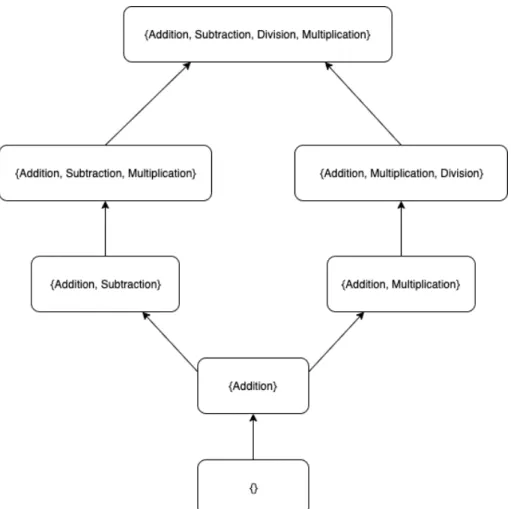
One idea of applying Machine learning in teaching is intelligent tutoring system (ITS) which can support student to improve their learning curve. In order to achieve this objective, re-searchers firstly have a consideration of learning the study structure of the study domain. This idea is based on an assumption that we can split the study domain into several compo-nents, and understand the interrelationship among them. In terms of this idea, the Knowledge space theory (KST) [1, 7, 9] provides us with a view on decomposition a knowledge domain into components and connect them as a graph of knowledge states to exploit the optimal learning path and assess the competencies of learners. In a certain domain of knowledge, the learning space is a finite set of items which could be learning objects; and all possible collections of items from the learning space are called the knowledge states. For example in a knowledge domain S, which contains summation,subtraction,division, and multiplication;
the corresponding knowledge states of this knowledge domain is presented in Figure 1.1. This theory has been successfully applied in many learning domains, such as mathematics and psychology. For instance, Goncalves presented the ideas of KST in mathematics; while Spoto et al. attempted to connect KST with psychological assessment in research [25]. However, there have not been many attempts to apply KST in the language fields. Learning logical subjects like mathematics bears a difference to linguistic learning. In linguistic field, learning concept witnesses more abstractions and complications.
1.2
Objectives
The main goal of this thesis is applying the KST to the domain of language learning to learn the student model and the domain model, with three major objectives:
2. Measuring the difficulty of concepts: the student model uses the performance of all stu-dents to learn the correlation between mastery states, mean scores, and score variances, which gives an estimate of the difficulty of the concepts.
3. Proposing a learning plan for students: the domain model learns the “surmise” relation— the prerequisite relation—between concepts in the domain of language learning, to estimate the most suitable learning plan for students based on the history of their performance.
To learn the student models to estimate student’s proficiency state, we use two algorithms: BKT and Threshold-based (Section 3.1). The learnt model is able to estimate the proficiency state (mastery state) of students on concepts based on their performance. The state of one student on one concept is labeled “learnt” or “not learnt”. Estimating the state means estimating whether a student has mastered one concept. The student model can also learn the mean score and variance of score of each concept, which mean the student model can help us measure the hardness of concepts.
To learn the domain model, we construct a surmise graph of the domain as a Bayesian network with each node manifesting for one corresponding concept. Bayesian network is a probabilistic graphical model, which encodes the conditional dependencies among a set of variables in a directed acyclic graph. In the domain of learning Russian, the items are called concepts such as “Negative construction”, “I conjugation”, “Negative sentences”, . . . . We apply five different algorithms (Section 5) to learn the structure of surmise graph from data. The surmise graph encodes the surmise relationship among concepts in topological order. The graph is able to suggest the optimal learning curve for students based on their current proficiency state and their target of study.
The domain model is able to suggest the optimal learning curve given the proficiency states of students of all concepts. The student is able to estimate the proficiency states of students of all concepts as the input of the domain model. By the domain model and student model, we can build a tutoring systems, which has the abilities to track the advancement of students, predict future performance of students, measure the hardness of concepts (feature of the student model), and provide the optimal learning curve for students (feature of the domain model).
background review for all solutions and ideas used in this thesis are denoted. Section 4 presents related works with this paper. It is followed by a description of our solutions in Section 5. The empirical experiments of all solutions and methodologies are then presented in Section 6. Section 7 is the place for discussion of current obstacles and future ideas for this topic. The last part of this thesis, Section 8, contains the conclusion along with the summary of the whole paper and the acknowledgement. The final concept graph along with the concept list and their information can be found on appendix pages.
All data for this thesis are collected from the Revita system which is a language learning platform developed by the cooperation between Computer Science department, Modern Lan-guages department of University of Helsinki and Foreign LanLan-guages and Literatures depart-ment of University of Milan [12, 13]. Revita is a part of ICALL, Intelligent Computer-Aided Language Learning created to support language education over many universities and orga-nizations in the world.
There are about 5000 questions distributed over 88 concepts and 6 levels of the Common European Framework of Reference for Languages (CEFR) system which are A1, A2, B1, B2, C1, and C2. Those concepts along with their CEFR information are provided by linguistic experts in Russian, for instance, teachers from Russian departments. The samples of student performances are collected directly from real Russian learners on Revita system. There are about 500 students having done one or many tests and approximately 4000 test sessions in total. In each test session, the time is limited and all concepts are asked with a randomized number of questions sampled from the corresponding question bank; however, it is unneces-sary that students answer all given questions in a test session. There are approximately 300 questions in each test in such way that each question belongs to only one concept and all concept is presented in each test session with at least one question. The timestamps, student identity numbers, and question CEFR levels are also recorded along with all questions in each test session.
2.2
Data Pre-processing
This thesis presents two experiments, the first using the original 88 concepts without taking into account their CEFR levels, and the second using a combination of concepts with CEFR levels. For example, concept “6, Lexicology. Lexical semantics” is distributed over three CEFR levels: B1, B2, and C1. In the second experiment, this concept is considered as 3 different concepts “6B1”, “6B2” and “6C1”. The total number of these “refined” concepts produced by this combination process is 127. Thus we have two experiments:
the models tracking student’s advancement. In the second step, we use the models trained after the first step to estimate the corresponding advancement states. Lastly, we recover the interrelationship between concepts based on the estimated advancement data from the second step. To do so, the accumulated examples are split into three disjoint datasets by grouping the students. The three disjoint datasets are:
• the “student” set (188 students, 1265 test sessions) used for training the student model, • the “domain” set (189 students, 1489 test sessions) for constructing the domain model,
and
• the “evaluation” set (189 students, 1255 test sessions) for evaluating.
Data of the first student group are used for step 1 in which the student models are built. The student models learnt from the first group are utilized to estimate state data of the second student group. Then, the state data of the second group is used to learn the concept graph (the knowledge structure). The third group is the evaluation data-set for the concept graph.
2.3
Data Table Format
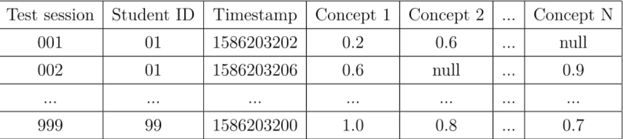
The samples after pre-processing are accumulated by test sessions. Each session is identified by test session ID and contains not only the score of all involved concepts but also timestamp and student number. The score of each concept is from 0.0 to 1.0 which presents for the
percentage of correct answers. If there is no response on one concept, the score information is marked as null value. The illustration of data table is displayed in Table 1.
Since we have two different configurations for concepts in domain of learning Russian which are concepts without CEFR and concepts with CEFR as mentioned above in Section 2.2, there are two data tables corresponding to two concept configurations.
Test session Student ID Timestamp Concept 1 Concept 2 ... Concept N 001 01 1586203202 0.2 0.6 ... null 002 01 1586203206 0.6 null ... 0.9
... ... ... ... ... ... ...
999 99 1586203200 1.0 0.8 ... 0.7
Knowledge space theory (KST) is a framework for identifying the learning structure of a knowledge domain. This theory was invented by Doignon & Falmagne in 1985 [9] and then improved by Albert & Lukas in 1999 [1]. The theory assumes that in a certain study field, there is a finite setQ of problem types, skills or concepts representing some learning objects
or levels in that knowledge domain; and set K which contains some subsets of Q. For
illustration, a student needs to master basic knowledge of number in order to understand some mathematical formulas and be able to handle all basic operations such as addition, subtraction, multiplication and division in a simple equation. Therefore, the study domain of solving a simple equation could be decomposed into two concepts: numbers and operations. However, there are some subsets of Qare not knowledge states (not belong toK) since these
subsets are not likely to exist. For example, one student cannot understand gradient without any knowledge about number and operations, hence there is likely no knowledge state contains gradient without numbers and operations.
The collectionKof subsets ofQwhich includes the empty set and theQitself is considered as
the set of knowledge states of the study domain. All elements of K are related to each other
in a topological order and together they construct a Bayesian network (Section 3.2) that the root node stands for the empty knowledge state and the last node stands for a knowledge state which contains all skills in Q. This Bayesian network is named the knowledge state
graph describing the study domain. For illustration, Figure 3.1 presents an example graph of a knowledge structure with Q= {X, Y, Z}. In KST, set K and set Q define the domain
model of a study field which is the first objective of an ITS.
To discover Q and K, there are some definitions that have been denoted by Doignon and
Falmagne in paper “Knowledge space and learning space” [8]. Firstly, the discriminative definition that for all conceptsXandY, the two collections of all knowledge states containing X or Y are identical if and only if X is equal Y. The second definition relates to learning
smoothness that if a knowledge state A contains knowledge state B then there is at least
one topological path to reach AfromB by learning concept one by one. The third definition
states learning consistency which implies that understanding more concepts does not limit learning new things. For example, if there is a state A contains state B and state B ∪ {q}
Figure 3.1: Knowledge structure graph with Q ={X, Y, Z}[7]
where q is a concept; then A ∪ {q} is also a state. The last definition, which is named
“antimatroid”, refers that every state in K except the empty state is able to be downgraded.
A state Ais able to be downgraded ifAcontains some concepts q thatA\ {q}is also a state.
There are many ideas to extract K or the knowledge state graph from students’ test results
such as the maximum residual method [19] or the distributed skill maps [26]. These methods introduce a term named response pattern. A response pattern is a unique pattern of answers
from students for one set of questions. One pattern can be responded by one or many students; therefore, the frequency of each pattern play is commonly utilized to infer the knowledge state graph for a group of questions or concepts. The maximum residual method takes the frequencies of student’s response patterns into account in order to find the most likelyK, while the distributed skill maps solution tries to construct a skill map from response
pattern and then derive the most probable knowledge state graph. The common point between those methods is trying to extract the K and knowledge state graph from response
patterns. However, we don’t know how many subsets of Q belong to the set K; therefore
the size of K is not known as well. In the worst case, the size of K could be 2n where n is
the number of concepts. In order to reduce the size of the graph, rather than discovering the knowledge state graph, we try to discover the surmise graph of concepts, which we define
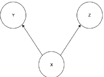
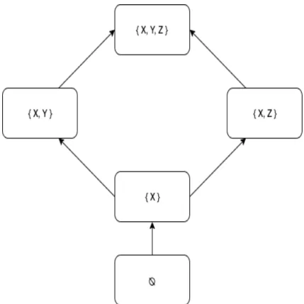
Figure 3.2: Example surmise graph given Q ={X, Y, Z}
The surmise graph of concepts is an alternative way to present the interrelationship among concepts in Qwhile ensuring the above definitions in KST, and it is also impossible to
trans-form to the knowledge state graph. The surmise graph is a Bayesian network (Section 3.2) as well with each node representing one concept. The direction edges between these nodes standing for their surmise relationship. Figure 3.2 is one simple instance of concept graph and Figure 3.3 is the corresponding knowledge state graph for Figure 3.2.
The target for the domain model is alternative to extracting the most probable surmise graph of concepts from students’ performance examples. We propose both theory-driven solution and data-driven solution. The theory-driven solution is based on prior theories that determines the topological surmise order of concepts. The data-driven methods such as the item tree analysis (Schrepp [22]) and Grow-shrink Markov blanket algorithm (Margaritis [14]) are capable to learn the statistical correlation and conditional probabilities among concepts from the given performance data. The detail description of both theory-driven and data-driven ideas are in the following sections on Bayesian networks.
3.2
Bayesian network
Bayesian network is a directed acyclic graph (DAG) that encodes all conditional indepen-dencies between a finite number of variables and their probability distribution P graphically
as the minimal I-map (Independency-map). An I-map is a DAG, which encodes all indepen-dencies of one probability distribution. Pearl [16] defined that a DAG Gis guaranteed to be
an I-map of a probability distribution P if every conditional independence encoded in G is
also valid in P. By the minimal I-map, we mean an I-map ofP which can be considered as
Figure 3.3: The knowledge state graph corresponding to Figure 3.2 invalidating the above rule on the distribution P.
One important note is that an I-map or Bayesian network can only maintain the conditional independencies in P, and the I-map that is valid for both conditional independencies and
dependencies is called D-map of the distribution P. However, much research follows the
faithfulness assumption that a networkGand distributionP are faithful to each other when
all conditional independencies inP are entailed by the Markov property onG. We also follow
this assumption throughout this thesis. Figure 3.4 is an example of a Bayesian network with the conditional probabilities.
D-separation. D-separation is a criterion to identify the conditional independencies in a DAG. D-separation determines whether two variables X and Y in a DAG are independent
given the evidence of several other variables in G, or unconditionally independent. This criterion detects the independencies by checking whether there are any unblocked paths (see
below) betweenX andY. In a DAGGof a probability distributionP, if there is no unblocked
path between X and Y, we can say that X and Y are independent in G and P.
Graph G only ensures the conditional independencies of the variables. The dependencies in G are not faithful to the probability distribution P. If there is at least one unblocked path
Figure 3.4: Example of Bayesian network [15]
Figure 3.5: d-separation example
Following to the faithfulness assumption that the dependencies in graph G is faithful to P,
we also can say that X and Y are dependent in P if there is at least one unblocked path
between two variables X and Y inG.
In unconditional cases, the path in a graph is a sequence of edges, disregarding their direction. A path is considered unblocked when there is no “head-to-head” pair of edges with respect to the direction. This rule assumes that the direction of each edge stands for the passing line of information in the network, and any colliders that block the flow of information also separate the dependencies. For instance in Figure 3.5, path X →Y →Z and U → T →Z
are unblocked but X →Y →Z ←T ←U is blocked by the ”head-to-head” collider of two
edges Y →ZandT →Z. Hence, X and U orX and T are not d-connected, while X and Y
or X and Z is d-connected, given no conditions, which can be written as X ⊥ T, X ⊥ U, X 6⊥Y and X 6⊥Z.
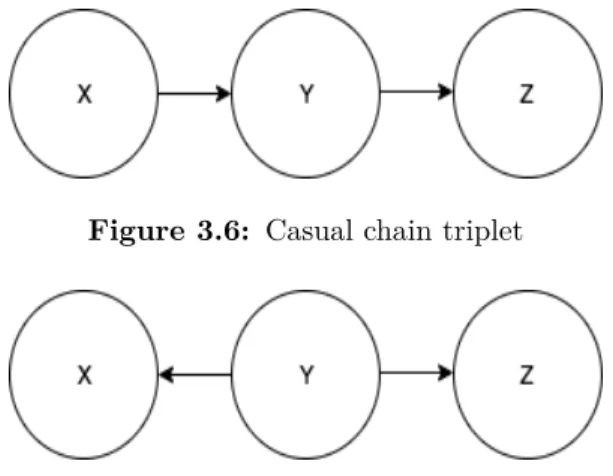
Figure 3.6: Casual chain triplet
Figure 3.7: Common cause triplet
path is blocked or not blocked by three rules on three types of variable triplets. By a triplet, we mean a set of three variable nodes which are linked directly, disregarding the direction. A path is considered blocked when it contains at least oneinactivetriplet (see below), and a
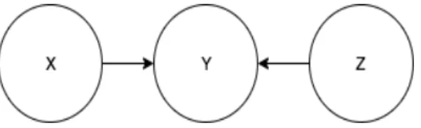
pair of variables is conditionally independent if every path between them is blocked. Three different types of triplets and their corresponding rules are: casual chain, common cause and common effect (v-structures), explained below, Figures 3.6, 3.7, 3.8.
A variableX is conditionally independent of all its non-descendant variables when the values
of its parent variables are observed. In terms of the first type, this means if we can observe the middle variable in the causal chain of three variables, then two remaining variables are independent. For instance in Figure 3.6 we have that X and Z are independent given Y or
we can say the evidence of Y makes the path fromX toZ inactive, written as X ⊥Z|Y.
The second rule for the “common cause” triplet implies that two variables are conditionally dependent if the common parent is observed while they are dependent without any conditions. For the triplet in Figure 3.7, we can say thatXandZare d-separated givenY, or the evidence
of Y blocks the path from X to Z; we say in this case that the triplet (X, Y, Z) isdeactivated.
In contrast to two above types, we know that if there is no evidence in the third type of triplet then two variables sharing same child are independent since there are “head-to-head” pair of edges between them. They are conditionally dependent with respect to the evidence of the common child. In the case of Figure 3.8, we can say that X and Z are independent
without given Y and dependent with given Y, or the evidence of Y unblocks and makes the
path from X toZ active.
Learning Bayesian networks. Bayesian network has been applied in many scientific fields such as biology, psychology, health care and physics, due to its ability to visualize the interrelationship between science concepts and phenomena. In situations where we have
Figure 3.8: Common effect triplet
inherent knowledge about the structure of the network, the parameters to fit the given data can be estimated by calculating the conditional probability among variables. In problems where we do not have a fixed network structure, it is possible to recover the network structure following some prior theories, or we can learn the structure directly from data. However, learning Bayesian networks from data is a challenging problem.
Learning parameters of Bayesian network. We can learn the parameters of the net-work with a fixed structure by applying the Bayes theorem. There are a wide variety of versions for the mathematical formula of Bayes theorem, but the most popular one is defined as
P(A|B) = P(B|A)P(A) P(B) .
In learning network parameters, we replace A by θ, and B by D and G, where θ stands for
the parameters of the Bayesian network, D presents the given observed data, and G is the
given graph structure. In case the structure is fixed, G does not play a pivotal role here.
Now, the model formula to estimate the Bayesian network parameters is
P(θ|D, G) = P(D, G|θ)P(θ)
P(D, G) (3.1)
or
P(θ|D) = P(D|θ)P(θ)
P(D) . (3.2)
In both Formula 3.1 and Formula 3.2, theP(θ) is the prior,P(D|θ) is the likelihood , which
represents the probability that D occur givenθ, and P(θ|D) is the posterior probability for
parametersθ with respect to dataD. The objective is to find the best-fit parametersθ to the
data D, which is equivalent to maximizing the posterior P(θ|D). Therefore the probability P(D), could be ignored. We can rewrite the formula as follows:
is useful to avoid overfitting in the situation when we have limited examples. Maximizing
P(θ|D) is equivalent to maximizing P(D|θ)P(θ) according to Formula 3.3. Maximizing P(D|θ) can be solved by Maximum Likelihood Estimation (MLE). MLE is equivalent to MAP
if the prior P(θ) is uniform, which means maximizing P(θ|D) is equivalent to maximizing P(D|θ).
Learning the structure of Bayesian network. In the literature, there are two basic data-driven solutions to extract the structure of the Bayesian network from data. The first solution is a score-based method [28]. This method assigns a formula to calculate a score for each version of the graph. The formula for the score usually describes the fitting of the graph to the observations, which is presented in Formula (3.4).
Score(G, D) = P(G|D), (3.4)
where Grepresents one version of network structure and Dis the data. We can apply Bayes
theorem here to expand Formula 3.4) to Formula (3.5.
Score(G, D) = P(G|D) = P(D|G)P(G)
P(D) . (3.5)
In order to find the greatest score, we need to find structure Gthat maximizes the P(G|D).
The denominator P(D) does not depend on G; therefore, the maximization depends on
the numeratorP(D|G)P(G). In the numerator, the probability distribution ofGis our prior
knowledge onG, and we assume thatP(G) is uniform and can be ignored. Hence, maximizing P(D|G) or P(G|D) results in the optimal score.
The second approach is constraint-based method [28], which constructs the network structure based on the status of conditional independence to learn the relationship among each pair of variables. We need to follow the above faithfulness assumption of Bayesian network for this method. The core component of this idea is the conditional independence test Ind(Xi;Xj|S)
to check the independence between Xi and Xj given the evidence S. According to the
faithfulness assumption, ifInd(Xi;Xj|S) returns that two variablesXi andXj are dependent
(or independent) given the evidence ofS, thenXiandXj are not d-separated (or d-separated,
respectively) given the evidence of S. This method can be exemplified by SGS algorithm
Those methods search for the best fit version of structure on data where the possible number of structures is 2n, where n is the number of variables in the domain. For instance, the SGS
algorithm computes the independencies for each pair of variables X and Y, with respect to
all 2n−2 subsets of set Q, containing all variables in the domain except the two variables
X and Y. Those methods with exponential complexity are impractical in our situation,
when our domain is comprised of up to 127 variables (Section 2.2). Therefore, we introduce two alternative methods in the thesis. The first is a version of the score-based method, which is modified to find an approximate answer to save computation time. The second is an independence-based algorithm, called the Grow-shrink Markov blanket algorithm, which exploits the properties of the Markov blanket in a Bayesian network.
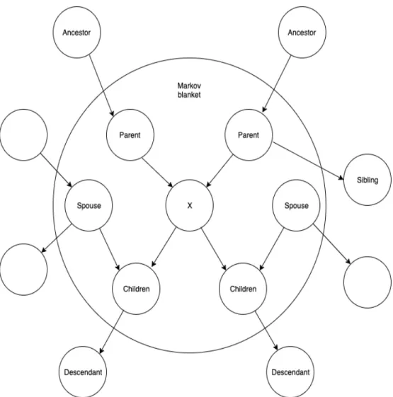
Markov blanket. For Bayesian networks in particular and directed acyclic graph in gen-eral, the Markov blanket of a nodeX in the graph is defined as the set of its parents, children
and spouses, where the spouses are the nodes that share the one or more same children with X. More detail on Markov blanket can be found in the paper “Probabilistic Reasoning in Intelligent Systems: Networks of Plausible Inference” published by Pearl in 1988 [17]. Fig-ure 3.9 is an example of Markov blanket for variable X. The evidence of X’s parents block
all paths from all ofX’s ancestors (except X’s parents) to X with respect to the first rule of
d-separation, while the second rule of d-separation declares that the evidence of X’s parents
also blocks all paths from X’s siblings, where the siblings are nodes sharing one or more
common parents with X. The evidence of X’s children blocks all paths from X to X’s
de-scendants (except X’s children) due to the first rule. The evidence of spouses ofX makes all
paths from allX’s children to all outside nodes of the Markov blanket inactive. Accordingly,
we have that for each variableX in the network if we can observe all variables in its Markov
blanket then this variable X is independent of all other variables in the graph. In other
words, the Markov blanket is all we need to predict the information of that node.
3.3
Grow-shrink Markov blanket algorithm
The Grow-shrink Markov blanket algorithm is described by Margaritis in his doctoral thesis [14]. He indicates that the algorithm focuses on the usage of Markov blanket in reconstructing the network structure. According to the above definition of Markov blanket, we have that all variables (except the spouses) in a Markov blanket of a variable X are the direct neighbors
Step 1—Markov blanket estimation. First, we need to estimate the Markov blanket for each variable. There are two main phases to do so, which are “Growing phase” and “Shrinking phase”. Margaritis [14] defines these phases as the following pseudo-code:
Algorithm 1 Pseudo-code to extract Markov blanket 1: 1. Initialization:
2: S ← ∅
3: U ← All variables in domain, 4: X ← considering variable 5: 6: 2. Growing phase: 7: while ∃Y ∈U − {X} such as X 6⊥Y|S do 8: S ←S∪ {Y} 9: end while 10: 11: 3. Shrinking phase: 12: while ∃Y ∈S such as X ⊥Y|S− {Y} do 13: S ←S− {Y} 14: end while 15:
16: 4. Return S as Markov blanket of X
According to the above algorithm, the growing step begins with an empty set S and keeps
adding into S the variables in the domain, except the considered variable that is dependent
on X with respect to current content of S. This phase simple tries to find a subset S of all
variables which does not violate the property of Markov blanket, that a blanket of a variable should isolate it to other variables. However, this first stage does not guarantee that S is
the Markov blanket of X; therefore the shrinking phase shrinks the redundant variables of S. The faithfulness assumption declares that any variableY in blanket ofX is dependent on X given the evidence of the blanket withoutY, or we can say Y and X is d-connected given Blanket(X)− {Y},∀Y ∈Blanket(X). The shrink phase filters out the redundant variable
in S that do not satisfy the above faithfulness assumption, then returns the Markov blanket
number of iterations that extend the setS without breaking the features of Markov blanket is n. Each iteration needs to check one conditional probability with respect to current content
of S which need to go over all input examples. Hence, the growing phase consumes O(n|D|)
time complexity. In the shrink phase, the size of set S is always smaller than the number of
variables in the domain, so checking all elements in setSneeds less thannloops. Similarly to
the growing step, the time complexity for each iteration isO(|D|) to compute the conditional
probability from examples. By summing up the time of both growing phase and shrinking phase, the time complexity to achieve one Markov blanket is O(n|D|+n|D|) = O(n|D|).
Here, the number of examples |D| could be omitted; resulting the time complexity is O(n)
which is linear time.
Step 2—Recover network structure. After identifying the Markov blanket for all vari-ables in the domain, Margaritis proposes his Grow-Shrink (GS) algorithm to use the estimated blankets to reconstruct the network structure. For each node X, the GS algorithm firstly
removes the spouses contained in the blanket of X, to collect the set of direct neighbors of X. To do so, the algorithm checks one by one variables Y in the Markov blanket to find
the spouses of X, all of which are unconditionally independent of X, and dependent on X
given the evidence of at least one subset of Blanket(X)− {Y}. After this step, we have the
neighbors ofX, but not the direction of the edges to the neighbors. In the next step, the GS
algorithm detects the direction of the edges by finding the parent nodes in each neighbor-hood, in such way that the evidence of X makes them dependent (Section 3.2). For a pair
of nodes, Y and Z, in the neighborhood of X, we have three possible configurations for the
triplet. Case 1 is v-structure (Y and Z are parents of X). The third rule of d-separation for
v-structure in Bayesian network says the evidence of a common child of two variables makes them dependent. Case 2: according to “casual chain” d-separation rule, if Y is parent while Z is a child ofX, then they are not dependent givenX. Case 3: ifY andZ are both children
of X, they are also independent given X.
After learning the parents, children and spouses of each node, we are able to identify the direction for edges in the network; however, there is no guarantee that there is no cycle in the structure due to the noise in sample data. The GS algorithm handles this problem by reversing the edge that belongs to the most cycles, and repeat this until no cycles remain. Lastly, the algorithm directs all edges that have no direction to complete the Bayesian network structure (without creating new cycles). The pseudo-code of GS algorithm [14], shown in
isO(n), wheren is the number of variables in the domain. Therefore the time complexity to
compute Markov blanket for all variables is O(n2). If b is the length of the biggest Markov
blanket, b is always smaller than the number of all variables n. The set T in each iteration
Y ∈ B(X) of step 2 has the maximum size b, so there are at most 2b subsets S of T. Therefore, the time complexity to compute the set of directed neighbors for all variables is
O(nb2b). The time complexity for step 2 in the worst-case scenario isO(n22n) with respect to
max(b) = n. In step 3, the maximum length of the neighbor set of one variable is alsob since
∀X : N(X) ⊂ B(X). Similarly to step 2, there are 2b different combinations of S∪ {X},
therefore computing step 3 takes O(nb22b). In order to detect cycles in the structure, the
Depth First Search (DFS) traversal algorithm can determine whether or not one edge is in cycle in O(n+m) time complexity where n is the number of vertices and m is the number
of edges. Hence, the time complexity to detect all cycles in graph is O(m(n+m)), where m
is at most n2. Finally, the algorithm iterates over all edges with O(m) time in the last step;
however this step can be done along with DFS traversal. The time complexity of combination of step 4 and 5 is O(nb(n+m)). By summing up all the steps, the total time complexity for
the whole algorithm isO(n2+nb2b+nb22b+nb(n+m)) = O(n2+nb2b+nb22b+n2b+nbm) = O(nb22b+n2b) or O(n2+nb2b +nb22b+mn+m2+m) =O(n2+nb22b). By assuming b is
a constant, the time complexity of GS algorithm is O(n2) which is practical.
The biggest advantage of the GS algorithm is its computational speed, because the number of conditional independence tests required in GS is lower than in the greedy algorithm. This benefit is shown through the time complexity which are O(n2) and O(2n) for GS algorithm
and greedy algorithm respectively. However, there are some uncertainties about the GS algorithm that the Markov blankets could be incorrect due to the limitations of sample data. The number of training observations is limited, and those observations are not able to completely represent the real interrelationship among variables; this could result in the wrong conclusion of conditional independence tests. The step computing the parents for each node is not applicable for nodes, which have a single parent or multi-connected parents. The GS algorithm resolves this problem in the last step, which orients the non-directed edges without generating cycles. The algorithm also deals with the cycles with the minimal number of edges needed be reversed. Margaritis [14] also presents an alternative algorithm named “Randomized Version of Grow-Shrink Algorithm” to resolve this problem. However, this updated version of GS algorithm is not applied in the scope of our paper yet.
3: for each X ∈U do
4: Calculate Markov blanket of X: B(X)
5: end for
6: [2. Compute direct neighbors] 7: for each X ∈U do
8: Initialize the neighbor set of X: N(X)← ∅
9: for each Y ∈B(X) do
10: Compute setT as the smaller set between B(X) - {Y} and B(Y) -{X} 11: if X 6⊥Y|S ∀S ⊂T then 12: N(X)←N(X)∪ {Y} 13: end if 14: end for 15: end for 16: [3. Compute parents]
17: for each X ∈U and Y ∈N(X)do
18: for each Z ∈N(X)−N(Y)− {Y} do
19: Compute setT as the smaller set between B(Y) - {X, Z} and B(Z) - {X,Y}
20: if ∃Z that Y ⊥Z|S∪ {X} ∀S ⊂T then 21: Orient Y →X (Y is parent of X) 22: end if 23: end for 24: end for 25: [4. Remove cycles]
26: while there exist cycles in network do
27: Compute set R containing all edges in all cycles with duplication 28: Reverse edge with the highest count of appearances in R
29: end while
30: [5, Complete the network] 31: for each X ∈U and Y ∈N(X)do 32: if X−Y is not oriented then 33: Orient X →Y
34: end if 35: end for
Figure 3.10: Example of Hidden Markov model [11]
3.4
Hidden Markov model (HMM)
Hidden Markov model (HMM) and Bayesian network are probabilistic graphical models, which are represented in a DAG. The basic idea of HMM is based on Markov chain. Gagniuc [11] defines that Markov chain is a model encoding the probability of a sequence of variables, where each variable is drawn from some set of variables. This technique is useful to predict the future of a sequence with respect to the current state. Markov chain is built based on the Markov assumption, that the probability of one variable in a sequence depends only on the previous variable. In other words, the present is the only matter, which impacts predicting the future.
Markov assumption: P(Xi|X1, X2, ..., Xi−1) =P(Xi|Xi−1).
HMM is an extension of the Markov chain which has a sequence of hidden states, which can be estimated by observing the process of emissions. An HMM is described byN—the number
of possible values of the hidden state (a finite number), and 3 sets of parameters—probability distributions:
1. I - initial state probability distribution,
2. E - emission probability distribution given the state,
3. T - transition probability distribution matrix given the state.
HMM is widely used to find the most probable sequence of hidden states given the sequence of observations of emissions.
[4], and has been applied widely in ITS field. The fundamental idea behind a BKT model is a hidden Markov model. Our purpose for a student model is to predict students’ mastery state on one skill through their performance in multiple tests, where the observed results over tests are the emission of their state. In our BKT models, the hidden variables are the mastery states, representing whether student has “learnt” or “not-learnt” a specific skill, while the emission variables are the performance over time of student on that skill. By assessing the students’ performance over time, the BKT models can monitor whether the student has understood the skill at each test session. The models also can predict the students’ results of that skill for the next upcoming test sessions, based on the latest performance of the student. Van de Sande [20] has summarized the properties of the BKT models that a BKT model consider the hidden states (mastery states) to have only 2 values, which are “learnt” or “not learnt”, with 4 parameters to optimize:
• P(L0) the probability that student has learnt the skill before the first attempt
(corre-sponding to distribution I in HMM)
• P(G) is the probability that a student has not learnt the skill, but luckily guesses the
correct answer (corresponding to distribution E in HMM)
• P(S) is the probability that a student has learnt the skill, but accidentally makes a slip
and gives a wrong answer (corresponding to distribution E in HMM)
• P(T) is the learning probability that present the chance a student can learn the skill
after one attempt. This P(T) is assumed to be constant over time (corresponding to
distributions T in HMM)
In this paper, we take into account the chance that a student can forget a skill that he has learnt with probability P(F) after one test session. The matrix
1 - P(T) P(T) P(F) 1 - P(F)
is the matrix of hidden state transitions. The state transition could be • learning the skill (from “not-learnt” state to “learnt” state), • forgetting learnt skill (from “learnt” state to “not-learnt” state)
Figure 3.11: BKT parameters diagram (1 means “not learnt”, and 2 means “learnt”. X-axis is the score on the concept, Y-axis is the density.
• or staying the same state.
We assume thatP(T) andP(F) are constant over time. Our target is estimating the mastery
state for each skill of students based on their performance on that skill over test sessions. Hence, instead of using sequences of questions with only “wrong” and “correct” responses (0 or 1), which are predicted by the state of mastery of the student and P(G) and P(S);
we use the list of test sessions, where questions are grouped by concept, with the emission values (in the interval between 0.0 and 1.0). The emission values are drawn from two normal
distributions representing the two hidden mastery states: “learnt” and “not learnt”. Con-sequently, the parameters of the BKT model become P(L0), P(T), P(F), µ and σ where
µ= [ µnot learnt, µlearnt ] and σ = [ σnot learnt, σlearnt ]. The emission probability distribution
P(E|S = learnt) and P(E|S = not learnt) now are calculated by the probability density
function of the normal distribution of each hidden state rather than based onP(S) andP(G).
The detail of connection between these parameters is presented in Figure 3.11.
The probability that a student has learnt the skill at each test session is dependent on the updated performance of that student; thus that probability at each test session is not constant over time. Letk be the index of the step (test session) in the sequence of test sessions;P(Lk)
is defined as the probability that the student has learnt the skill at the kth test session and
Ek defines the performance of student on that skill (0.0 to 1.0) at the kth test session. The
performance Ek is drawn from the corresponding normal distribution of the state at test
session k. Figure 3.12 displays the structure of a BKT model.
Figure 3.12: Bayesian Knowledge Tracing model
P(Lk) = P(Lk−1) (1−P(F)) + (1−P(Lk−1))P(T),
and
P(Ek) = P(Lk)P(Ek|Slearnt) + (1−P(Lk))P(Ek|Snot learnt),
where P(Ek|Snot learnt) = exp (−(Ek−µ1)2 2(σ1)2 ) σ1 √ 2π , and P(Ek|Slearnt) = exp (−(Ek−µ2)2 2(σ2)2 ) σ2 √ 2π .
Given the emission sequence E, the log-likelihood of E, P(E) is calculated as P(E) = YP(Ek), f or all k,
or
log(P(E)) =Xlog(P(Ek)), f or all k,
where Ek is the observed test results of the student over test sessions. We can maximize the
log-likelihood of the sequence of emissions, log(P(E)), by applying the Expectation
model and the domain model. The student model is used to track the advancement of the proficiency level of students on concepts. The domain model is used to represent the structure of the knowledge domain and the connections among all concepts.
Bayesian Knowledge Tracing model is one common technique to track the advancement of proficiency levels (knowledge states) of students over test sessions based on the students’ performance. The standard BKT contains 2 knowledge states which are “learnt” and “not-learnt”, and probabilities to determine the advancement process [bkt˙related]. Yudelson et al. [bkt˙related] present a promising result for applying BKT on estimating individual knowledge advancement. Zhanga and Yao [29] introduce an update version of the BKT, which has the name is three learning states BKT (TLS-BKT) with 3 states “not-learnt”, “learning” and “learnt”. They believe that the TLS-BKT has a better performance than the original BKT with 2 states. The common point between BKT and TLS-BKT is that they both ignore the probability of forgetting. In this thesis, we utilize the standard BKT with 2 states, but we take the forgetting into account to track the knowledge states of students. There are many solutions have been proposed to learn knowledge structure as a corresponding knowledge state graph such as BLIM [10], distributed learning object [26], or maximum residuals method [19]. One popular mechanism to construct knowledge state graph is using the frequency of response pattern from student’s answers. The BLIM algorithm which is invented by Falmagne and Doignon in 1988 attempts to select the most probable knowledge states belong to knowledge structureK. To access the states, the algorithm takes into account
both conditional probability and frequency of knowledge states and answer response patterns from students to find the most likely set of knowledge states that generates the observed responses. Schrepp [23] proposes a method to determine which response pattern is belong to the knowledge domain. He assumes that a response pattern could be generated from one knowledge state in domain in order find an optimal frequency thresholdLin such way that all
response patterns arriving more than Ltimes are considered as knowledge states in domain.
However due to the probability of lucky guess or careless mistake, the frequency non-state-patterns are possibly higher than some state-non-state-patterns. To handle this issue, Robusto and Stefanutti [19] proposed a mechanism that appends new factor named expected frequencies of the response patterns. This expected frequency are able to be obtained by BLIM algorithm [10]. The common point of all the above methods is around observing the frequencies of
graph could be exponential (Section 3.1).
To alter the knowledge state graph in order to represent the study domain, the surmise graph of concepts is a decent candidate where the skill map is still able to encode the sur-mise relationships among skills in domain as well as be easily converted to knowledge state graph. Desmarais and Gagnon have introduced quite similar idea in their research on learn-ing knowledge structure as item graph [6]. They attempt to present a knowledge domain in form of a Bayesian network presenting the item to item structure. By the item to item structure, they mean a DAG structure that represents all surmise relationships between all individual items in the domain. To do so, they propose two approaches. The first approach learns the corresponding Bayesian network on observed data with K2 algorithm [3] and PC algorithm [24]. The second approach believes that the knowledge items in a study domain are in surmise relations following a partial order in which some skills should be mastered before the others. They utilize this topological theory in order to iterate over all pair of items to find the surmise relation in each pair. They consider that itemA itemB (the mastery of B precedes the mastery of A) if the following conditions are satisfied
P(B|A)≥pc,
and
P( ¯A|B¯)≥pc,
and
P(B|A)6=P(B),
where A and B stands for “mastering” itemA and item B while ¯A and ¯B presents for “not
mastering” these items. They experiment their theory with pc= 0.5.
Hou et al. [12] try to learn the study domain as a skill map structure with Elo-based methodology. Their result skill map is flattened, therefore the size of corresponding state structure is exponential if we try to recover it. Those works of learning item to item structure or the surmise graph of concepts deduces that it is possible to understand the study domain as a surmise graph in which learning surmise graph is more achievable in some scenarios. Because our second objective is learning the surmise graph, which is a Bayesian network, from the mastery data; algorithms for Bayesian network learning also can be used to construct the domain model. Yuan and Malone [28] show that there are three main approaches to learn a
network structures in solution space. The constraint-based learning is able to scale the large dataset but vulnerable to the noises. The hybrid learning is the integration between the advantages of two base learning methods: score-based learning and constraint-based learning. To reduce the running for score-based learning, Yuan and Malone [28] present a dynamic programming approach, which constructs the order tree and then they use a search algorithm such A* to find the optimal path to the best network structure. By the order tree, they mean a state space graph for learning Bayesian network, which has the most-top node is a network structure with only one random node (a start node) and the most-bottom nodes are the network structure with all involved nodes. In terms of constraint-based and hybrid learning, Margaritis [14] presents two solution: Grow-shrink Markov blanket algorithm and Randomized Version of Grow-Shrink Algorithm, which try to identify the conditional independence relations from the data to construct the network structure.
the corresponding domain model and student model with three main objectives). The student model is also used to estimate the mastery data, which is the input for learning the domain model.
To learn the domain model, we apply Greedy algorithm and two Bayesian network learn-ing libraries, which are Gobnilp (Globally Optimal Bayesian Network learning using Integer
Linear Programming) [5] and pomegranate [21] as baseline algorithms. We also apply GS
algorithm and Theory-based algorithm to compare with three baseline algorithms (Greedy algorithm, Gobnilp, pomegranate).
To learn the student model, we usehmmlearnlibrary in Python [27] to learn the BKT models
because the basic idea of BKT models is Hidden Markov Models. We use GaussianHMM
class to construct the HMM of our BKT models since we assume that the score of a mastery state (“learnt” or “not-learnt”) is a variable with normal distribution (Gaussian distribution). The methodology flow is displayed in Figure 5.1. The student model (BKT models or Threshold-based estimator) estimates the mastery state data for the input score data. The estimated mastery data is the input for one of three GS, Greedy score-based, Theory-based algorithm, Gobnilp library and pomegranate library to learn the surmise graph of concepts (the domain model), which represent the domain of learning language. We have 10 con-figurations of the methodology to learn the student model and the domain model, which are BKT-GS, BKT-Greedy, BKT-Theory, BKT-Gobnilp, BKT-pomegranate, Threshold-GS, Threshold-Greedy, Threshold-Theory, Threshold-Gobnilp, and Threshold-pomegranate. According to Section 3.1, the domain model of a knowledge space is an Bayesian network, which encodes the surmise relationship among concepts in the domain, and the student model contains a BKT model for each concept, to estimate the proficiency level by tracking students’ performance. Section 2.2 presents that there are 88 concepts, which are distributed among six levels of CEFR; therefore we we have two different sets of concept to represent the knowledge space. In this thesis, we experiment with the KST on both two sets of concepts.
Figure 5.1: Methodology flow
5.1
Learning student models
The function of the student model is analysing the test result of students and assessing their mastery state on each skill in each test. We propose two mechanisms to learn the student model that can estimate the proficiency levels of students based on their sequence of performance. Both techniques are applied the “student” data set.
5.1.1
Threshold-based model
The first is a naive approach, which determines the mastery state by a mastery threshold, θ,
(a hyper-parameter, which we tune) on the performance of students for each skill. We say that a student has learnt the concept (mastery state) if their score on this concept is equal or higher than the mastery threshold. For example, if the score of student A on concept B
in test session C is 0.8 (or 0.6), and the mastery threshold θ is 0.7, then we consider that
student A has learnt (or not learnt) concept B, respectively, at the time of sessionC. More
detailed examples are displayed in Table 5.1 and Table 5.2.
Table 5.1 is a sample data table of score over N concepts in three test sessions. In the
data, each test session also includes the timestamp and student identity number; however that information is not used in this first approach. The corresponding state data table for Table 5.1 with respect to θ = 0.7 is presented in Table 5.2.
003 0.4 0.5 ... 0.7
Table 5.1: Example score data table
Test session Concept 1 Concept 2 ... Concept N
001 0 0 ... null
002 1 null ... 1
003 0 0 ... 1
Table 5.2: State data corresponding to Table 2 (withθ= 0.7)
This method ignores the time factor, and treats each test session as if it is done by different a individual, disregarding the student ID. Therefore, the first technique is simple with only one parameterθ (θ= 1−P(S)), which involves the probability P(S) that a student who has
learnt the concept makes accidental mistake/slip. In this thesis, the parameter θ is tuned
from 0.5 to 0.9, with an increment of 0.05, and the impact report is presented in Experiment
section.
5.1.2
Bayesian Knowledge Tracing model
The second approach utilizes the Bayesian knowledge tracing model that takes both the timestamps and the IDs of the students into account to estimate the mastery state. This solution treats test sessions in sequences in such way that they are grouped by student ID and ordered by timestamp. The mastery states on each concept are estimated by not only the performance of this concept on the current test session, but also by the previous sessions. We train one BKT model for each concept in the domain. The BKT model is used to learn the mastery state data, which is used to learn the surmise graph, for example, by the GS algorithm and other algorithms, in Section 5.2.
In a test sequence of one student on a single concept, there are originally five parameters that we want to learn, which are the probability, P(L0), that a student already learnt the concept
in the first attempt, the probability, P(L), that a student is able to learn the concept after
one opportunity, the probability, P(F), that a student forgets the learnt concept after one
The student models learnt by this step are used to predict the mastery state for the “Domain” dataset as the input for training domain model, as well as to estimate the mastery state data for the “Evaluation” dataset in order to evaluate the domain model (Section 2.2).
5.2
Learning domain models
The objectives of domain model is to encode the inter-dependencies among concepts in the domain. Section 3.1 mentions that the domain model is originally a directed acyclic graph of knowledge states (knowledge state graph), but it can be represented by a surmise graph of concepts. As mentioned in Section 2.2, we utilize the student models, which are learnt from thestudentdataset to estimate the mastery state data for thedomaindataset. The estimated
state data of the domain dataset is the input for learning the surmise graph of concepts. To
learn the surmise graph of concepts from mastery state data, we apply five solutions: GS algorithm, Theory-based algorithm, Greedy algorithm, Gobnilp library and pomegranate library. The Greedy algorithm, the Gobnilp library and the pomegranate library are baseline methods, which are used as options for comparison to the GS algorithm and Theory-based algorithm. The Gobnilp library [5] and the pomegranate library [21] are Python libraries to learnt Bayesian network from data. The methodology of experiment with the GS algorithm, the Theory-based algorithm and the Greedy algorithm is described as follows.
5.2.1
Theory-driven method
The first solution utilizes our prior assumption on the surmise relationship between concepts: the assumption is that for any pair of concepts A and B, 1. A and B are not connected by
a surmise relation, or 2. A is prerequisite for B, or 3. B is prerequisite for A. We believe
that some concepts are prerequisite for some other concepts in such way that all concepts connect to each other in a topological order. This assumption is based on the reference to the parital order knowledge structures (Desmarais & Gagnon [6]). The surmise relationship
between two concepts A and B is described in Table 5.3, where “+” represents for “learnt”
the concept and “-” for “not-learnt” the concept.
According to the Table 5.3, ifABthen the probability that a student has mastered concept B given that he has mastered concept A should be close to 100 percent. In other words,
- + compatible
- - compatible
Table 5.3: Compatibility of states ofAandB with the prerequisite relation between conceptsAB if you mastered the harder concept, you should have mastered the prerequisite concepts. If you are not able to understand the prerequisite concept then you are not likely to master the harder concept.
For every pair of concepts Aand B, this method follows the rules between concepts in Table
5.3 to check whether one concept is prerequisite for the other. To check the compatibility, we look up the input samples to calculate the corresponding conditional probability for each case in Table 5.3. Due to the uncertainty of estimated state data, we assume that the conditional probabilities are not zero and one. For example,P(Learnt B|Learnt A) does not need to be
1.0 to consider the first case is compatible. We use a threshold hyper-parameter φ in such a
way that P(Learnt B|Learnt A) should be equal or higher than φ (rather than equal 1.0)
or the probability P(N ot−Learnt B|Learnt A) should be lower than 1−φ rather than 0.0
to assess the second case as incompatible. Parameter φ is also tuned in range 0.5 to 1.0 with
step 0.05. The concept pairs that are not compatible the prerequisite connection indicate
these pairs of concepts have no surmise relation.
5.2.2
Greedy score-based data-driven method
The second approach is a score-based data-driven method, which tries to find the most probable surmise graph of concepts given the input mastery data. We start by the following formula for the score function
Score(G, D) = P(G|D) = P(D|G)P(G) P(D)
This function is mentioned in Section 3.2 whereGstands for a graph structure andDstands
for training data, which is the estimated mastery data. The goal is finding the structure G
that results in the highest value of score onD by maximizingP(G|D) or P(D|G), where the
distribution P(G) is uniform.
The probability P(D|G) can be factorized—written as a product of the individual density
Figure 5.2: Directed Acyclic GraphG0 can be presented as follows
P(D|G) =YP(Xv|G, P arent(Xv)), ∀v ∈Q
or
log(P(D|G)) = Xlog(P(Xv|G, P arent(Xv))), ∀v ∈Q,
where Q is the set of all concepts in the domain. Equation (5.1) is an example for network
factorization for graph G0 in Figure 5.2.
P(A, B, C, D) = P(A)P(B|A)P(C|A)P(D|B, C) (5.1)
According to the factorization of the likelihood P(D|G), we can maximize each part of the
factorization in order to achieve the greatest value for P(D|G). It can be done by trying
all parent configurations for each variable to find the best configuration for the greatest conditional probability, P(Xv|G, P arent(Xv)). This method iterates all possible structures
of the surmise graph to select the structure with the highest likelihood on the training data. However, we have 88 or 127 concepts, which means that the total number of possible structures is 288 or 2127 respectively. Therefore, this naive approach is not practical.
In order to reduce the time complexity, we use an alternative approach to trade-off quality for speed to search for an approximate structure. We start with a random structure and keep modifying it to boost the likelihood on data until we decide to stop. The modification at each iteration is possibly removing an edge, reversing an edge or adding a new edge. The algorithm selects the modification on each iteration that drives the factorization changes
ation. We experiment with this technique with several initial structures, which includes an empty network (DAG without any edges), a fully-connected network with randomly assigned directions, and some random networks (not empty and fully-connected).
5.2.3
Grow-shrink Markov blanket data-driven method
Grow-shrink Markov blanket algorithm, as described in Section 3.3, is another data-driven option to learn the Bayesian network structure. This algorithm has lower time complexity than the greedy score-based solution. In this paper, we also attempt to apply the GS algo-rithm [14] to learn the surmise graph of concepts. The detailed explanation of GS algoalgo-rithm can be found in Section 3.3. The running time and performance report for GS algorithm is presented along with two first solutions in Section 6.
network among 88 or 127 concepts. They utilize more than 32GB memory (our maximum
memory) and get stopped during the learning. Gobnilp is able to learn the network structure for maximum 20 concepts with respect to our resource. Pomegranate is able to learn the network structure for maximum 23 concepts with respect to our resource. On the other hand, the GS algorithm, Greedy score-based algorithm and Theory-based algorithm are possible to handle all 88 or 127 concepts with less memory usage (up to 16GB)
6.1
Concepts without CEFR
In this experiment, we attempt to learn the knowledge space for the 88 concepts, not using their CEFR information. The learnt surmise graphs are evaluated based on the evaluation dataset. The evaluation dataset has been transformed into mastery states by BKT model or Threshold-based estimator in Section 3.5 and Section 5.1.1. The log-likelihood is computed from the mastery states M(D) of the evaluation dataset given the surmise graph G, by logP(M(D)|G). The likelihood P(M(D)|G) is computed by following formula
P(M(D)|G) = YP(S|G), ∀S∈M(D),
whereSis one test session inM(D). The probabilityP(S|G) for each test sessionS inM(D)
is calculated by the factorization, as following formula
P(S|G) = YP(CS|P arent(CS)), ∀C ∈Q,
where Q is set of all concepts and CS is mastery state of concept C in test sessionS.
6.1.1
Bayesian knowledge tracing models
We train 88 BKT models for all concepts. The total time for training all models is ap-proximately 82 seconds, using 4 processors. The mean scores for the “learnt” state for each concept are mostly in the interval between 0.75 and 0.85, except concepts labeled “7”, “8”,
“191”, “230”, “85” and “89”. The mean scores for the “not-learnt” state are mostly in the interval between 0.1 and 0.3. There are two significant exceptions, which are concept “85”
![Figure 3.1: Knowledge structure graph with Q = {X, Y, Z} [7]](https://thumb-us.123doks.com/thumbv2/123dok_us/613392.2573498/14.918.268.644.122.515/figure-knowledge-structure-graph-with-q-x-y.webp)
![Figure 3.4: Example of Bayesian network [15]](https://thumb-us.123doks.com/thumbv2/123dok_us/613392.2573498/17.918.247.676.101.535/figure-example-of-bayesian-network.webp)
![Figure 3.10: Example of Hidden Markov model [11]](https://thumb-us.123doks.com/thumbv2/123dok_us/613392.2573498/27.918.225.697.125.290/figure-example-of-hidden-markov-model.webp)