Hans Manner
Estimation and Model Selection of Copulas with an Application to Exchange Rates
RM/07/056
JEL code: C13, C52
Maastricht research school of Economics ofTEchnology and ORganizations Universiteit Maastricht
Faculty of Economics and Business Administration P.O. Box 616
NL - 6200 MD Maastricht
Estimation and Model Selection of Copulas
with an Application to Exchange Rates
Hans Manner
∗December 19, 2007
Abstract
Copulas are the part of a multivariate distribution function that fully captures the cross sectional dependence between the variables of interest and they have become a very popular tool to model dependencies different from the linear correlation of elliptical distributions. We review the theory of copula functions, present a number of examples and describe how to sample random data from these. Different techniques for estimation and model selection are discussed and compared in an extensive Monte Carlo study. We find that a test not considered in the literature, namely the Jarque-Bera test applied on transformed data from the conditional copula, has the best properties of the presented tests, but that the most reliable criterion for selecting the best fitting copula is the Akaike information criterion. We model exchange rate returns of Latin American currencies against the euro with copulas and we find evidence of symmetric dependence, excess upper tail dependence and excess lower tail dependence.
Keywords: Dependence, Copulas, Semiparametric Estimation, Model selection. JEL Classification: C13, C52.
∗Department of Quantitative Economics, Maastricht University, PoBOX 616, MD 6200, Maastricht, The
1
Introduction
An assumption that is often made about the (joint) distribution of financial variables is that of normality. The dependence between variables that have a multivariate normal distribution is purely determined by the linear correlation coefficient. However, empirical findings show that asset returns have skewed and leptokurtic marginal distributions and that the depen-dence between these asset returns goes beyond the simple linear form. There is evidepen-dence that extreme co-movements (known as tail area dependence) occur and that some markets may be more dependent during extreme downward movements then when they are moving upwards. Simply looking at linear correlation in a non-elliptical world can be misleading as described by Embrechts et al. (2002). Copula functions allow for modeling joint multivariate distributions in a simple and extremely flexible way. Copulas are able to yield any kind of dependence structure independently of the marginal distributions. Whereas the bivariate Normal distribution requires its margins to be normally distributed as well, a Gaussian cop-ula is characterized by the correlation coefficient if the margins were normally distributed. They can take on any distribution, which need not even be equal for all the margins. This explains the simple algorithm for simulating data from a Gaussian copula, which simply requires imposing linear dependence on a number of normally distributed variables by pre-multiplying the series with the Cholesky decomposition of the desired covariance matrix and then using Fisher’s probability integral transform to give the marginals any distribution desired. Other copulas cannot be understood in such a simple way and they allow for very different types of nonlinear dependence. This may be depicted by graphing the relationship between the parameter of a given copula and the corresponding linear correlation coefficient, which will be a nonlinear one.
The Latin word ”copula” means ”link, tie, bond”. Copulas (or copulae when using the Latin plural) were first introduced by Sklar (1959), who proved the main result on copulas known as Sklar’s theorem. They offer scale invariant measures of dependence, so dependence is not affected by increasing transformations in any of the variables. Their use in econometrics developed over the last 15 years, but they become more and more popular as more useful applications in finance arise. One application where copulas turn out to be very useful is quite obviously the Value-at-Risk of a portfolio, as it might differ quite significantly when comparing its value under the assumption of joint normality and when having heavy tailed margins and a copula that allows for a higher dependence during market downturns (see for example Junker and May (2005). Copulas offer further applications in risk management like modeling joint defaults for credit risks or when pricing exotic options with two or more underlying assets. Cherubini et al. (2004) show many applications of copulas in finance. Further uses are the construction of investment portfolios and the more realistic simulation of asset returns. Another application suggested is modeling autoregressive dynamic processes
using copulas to capture the time dependence in one variable rather than the dependence between two or more variables as in Bouy´e et al. (2001). More mathematical treatments of copulas are the books by Nelson (2006) and Joe (1997) or Embrechts et al. (2003).
In this paper we aim at reviewing the theory needed to understand copula based modeling and apply it to a given data set. We focus mainly on techniques for simulating random observations from copulas, the different ways of estimating copulas and some simple model selection techniques. We contribute to the issue of model selection by showing that selecting the candidate copula that produces the highest Akaike information criterion is a very reliable method and that using the Jarque-Bera test on the appropriately transformed data performs better than some alternative tests that have been suggested in the literature.
The paper is structured as follows. The underlying theory is developed in Section 2, includ-ing some commonly used measures of dependence and the algorithms used to simulate data from a given copula. Furthermore we present the mostly used copula functions and their properties. The estimation and testing of a given copula model will be discussed in Section 3 and the performance of the different methods will be analyzed with the help of Monte Carlo studies in Section 4. In Section 5 their practical use will be illustrated by modeling the joint distribution of exchange rates of Latin American currencies against the Euro. Finally, we conclude in Section 6.
2
Introducing copulas and related concepts
A copula can be seen as a correspondence, which assigns the value of the joint distribution function to each ordered pair of values of the individual distribution functions. Alternatively it can be seen as the joint distribution function of a set of uniformly (0,1) distributed ran-dom variables or simply as a function, which couples, or joins, the marginal distributions with their multivariate distribution function. These ”operational” definitions serve as a good intuition about what a copula function is.
All results in this section are derived for the bivariate case. For an extension to the multi-variate case, which is only trivial for very few cases, see Nelson (2006). Also proofs for most of the results mentioned can be found there.
2.1
Preliminaries and copulas defined
Before we are able to introduce copula functions themselves a number of properties need to be presented. First of all the notion of a nondecreasing function has to be generalized for the multivariate setting. We begin by defining the concept of a 2-increasing function. Note thatR¯ denotes the extended real line.
Definition 2.1.1. Let S1 and S2 be nonempty subsets of R, and let H be a function such that DomH =S1×S2. Let B = [x1, x2]×[y1, y2] be a rectangle all of whose vertices
are inDomH. Then the H-volume of B is given by:
VH(B) =H(x2, y2)−H(x2, y1)−H(x1, y2) +H(x1, y1) (1)
A natural interpretation of the H-Volume is when H is a distribution function. It then rep-resents the probability of an event occurring in the region specified, which is a rectangle in the 2-dimensional case.
Definition 2.1.2. A 2-place real function H is 2-increasing if VH(B) ≥ 0 for all rect-angles B whose vertices lie inDomH.
We call a function from S1×S2 into R grounded if there is a least element in S1, as well
as in S2, let’s say a1 and a2, such that H(x,a2)=0 and H(a1,y)=0 for all (x, y) in S1×S2.
A function that is grounded and 2-increasing is known to be increasing in each argument. Another property that will be useful later on is the following. LetS1 andS2 have a greatest element, b1 and b2 respectively. Then the one dimensional marginals of H(x, y) are given
by F(x) = H(x, b2) and G(y) = H(b1, y). With this at hand we are ready to present the
definition of a copula.
Definition 2.1.3. A two dimensional copula is a function C from I2 to Isuch that 1. C is grounded and 2-increasing.
2. C(u,1) =u and C(1, v) = v (margins)
Hence a copula is no more than a function withI2 as its domain, Ias its range, and that is increasing in each element and has marginals.
The main result about copula functions is Sklar’s theorem (1959), which shows why copulas are so useful for modeling multivariate distribution function.
Theorem 2.1.4 (Sklar’s theorem for continuous distributions) Let F be the dis-tribution of X, G be the disdis-tribution of Y, and H be the joint disdis-tribution of (X,Y). Assume that F and G are continuous. Then there exists a unique copula C such that
H(x, y) =C(F(x), G(y)),∀(x, y)∈R×R (2) Conversely, if we let F and G be distribution functions and C be a copula, then the function H defined by equation (2) is a bivariate distribution function with marginal distributions F
and G.
In other words, the joint distribution can be represented separately by the marginal dis-tribution functions and the copula, which completely describes the dependence between the i.i.d. random variables X and Y.1 The converse turns out to be very useful in the
con-struction of multivariate distribution functions, as we now can take any pair of marginal distributions and any copula to construct a bivariate distribution. This allows for a large number of multivariate distribution functions that can be constructed easily.
There is a very useful corollary to Sklar’s theorem, which allows us to represent the copula by the joint distribution function and the inverses of the marginals. To ensure the existence of these inverses a new concept of the inverse of a function is required, which is called the quasi-inverse.
Definition 2.1.5. The quasi-inverse, F(−1) of a distribution function F is defined as
F(−1)(u) =inf{x:F(x)≥u} for u∈[0,1] (3)
Corollary 2.1.6Let H be any bivariate distribution with continuous marginal distributions F and G. Let F(−1) and G(−1) denote the (quasi-) inverses of the marginal distributions.
Then there exists a unique copula C from I2 to I such that
C(u, v) = H(F(−1)(u), G(−1)(v)),∀(u, v)∈I2 (4) The next result answers the natural question, whether there is an upper and a lower bound that holds for every copula.
Theorem 2.1.7 (Fr`echet-Hoeffding bounds inequality) Let C be a copula. The for every (u,v) in I2
W(u, v) = max(u+v−1,0)≤C(u, v)≤min(u, v) = M(u, v) (5) The upper bound corresponds to perfect positive dependence between two variables, the lower bound to perfect negative dependence. Additionally consider the function Π(u, v) =uv, which, not surprisingly, corresponds to independence. In the bivariate case these three important functions are copulas. For n≥3, however, the function W is not a copula. Finally, consider the function
ˆ
C(u, v) =u+v−1 +C(1−u,1−v), (6)
1The general discussion of the theory will be in an i.i.d. setting and we denote random variables by
which is the copula of a joint survival function. This is known as the survival or rotated copula.
As copulas are used to model dependencies one must specify of how to measure dependence. Traditionally the dependence between two random variables is measured by the linear corre-lation coefficient. However, when the dependence is not described by an elliptical distribution it can be quite misleading to use linear correlation and it might be more reasonable to use copula based measures of dependence, which are scale invariant (see Embrechts et al. (2002) for caveats on using the correlation coefficient for measuring dependence). One of these more robust copula based measures is Kendall’s tau. It has become the most popular measure of overall dependence in the literature on copulas and it relies on the concept of concordance. Consider two pairs of observations (xi, yi) and (xj, yj) from the continuous random variables (X, Y). We call these pairs of observationsconcordant if (xi−xj)(yi−yj)>0 anddiscordant if (xi−xj)(yi−yj)<0. Hence, two random variables are said to be concordant, when large values of one random variable are associated with large values of the other, and similarly small values tend to be associated with each other.
Using the concept of concordance we are now able to introduce a measure of association known as Kendall’s tau. Its sample version is defined as the fraction of concordant pairs of observations in the sample minus the fraction of discordant pairs of observations. The population version of Kendall’s tau is defined as the difference between the probability of concordance and the probability of discordance.
τ =τX,Y =P[(X1−X2)(Y1−Y2)>0]−P[(X1−X2)(Y1−Y2)<0] (7)
Kendall’s tau may be represented as a function of the expected value of a copula as follows.
τC = 4E(C(U, V))−1 (8) For some copulas there is a one to one relationship between its parameter and Kendall’s tau. Another frequently encountered and important dependence concept, which is relevant when modeling extreme events, is tail dependence. It measures the dependence of the random variables X and Y in the upper-right-quadrant and lower-left-quadrant. As the measure discussed above it is a copula property and hence it is invariant under strictly increasing transformations of the random variables. There are two alternative definition for the coeffi-cient of upper tail dependence. We first state the probabilistic one, followed by the definition in terms of copulas.
Definition 2.1.8 Let (X, Y)T be a vector of continuous random variables with marginal distribution functions F and G. The coefficient of upper tail dependence of (X, Y)T is
lim
u%1P[Y > G
−1(u)|X > F−1(u)] = λ
Definition 2.1.9If a bivariate copula C is such that lim
u%1
1−2u+C(u, u)
1−u =λU (10)
exists, then C has upper tail dependence ifλU ∈(0,1], and upper tail independence ifλU = 0. In a similar way the concept of lower tail dependence can be introduced. Only the defi-nition corresponding to defidefi-nition 2.1.9 is considered here.
Definition 2.1.10If a bivariate copula C is such that lim
u&0
C(u, u)
u =λL (11)
exists, then C has lower tail dependence ifλL∈(0,1], and lower tail independence ifλL = 0. Alternative formulas for λU and λL exists and can be found in Embrechts et al. (2003). There it is shown that the coefficient of upper tail dependence for a copula is equal to the coefficient of lower tail dependence for the corresponding survival copula and the other way around. We will encounter some illustrations of tail dependence in the next section, where some families of copulas are introduced.
2.2
Examples and families of copulas
In this section the most commonly used copulas will be described and their properties will be presented. The presentation is far from complete, but covers the copulas that are con-sidered in most applications in the literature. For exhaustive lists of copula functions and various methods for constructing copulas the books by Joe (1997) and Nelson (1999) may be consulted.
2.2.1 Elliptical copulas
Elliptical copulas are simply the copulas of elliptical distributions. They share a number of properties of the multivariate normal distribution and they are used to model multivariate extreme events and non-normal dependencies. As a result of the fact that simulations from multivariate elliptical distributions are easy to perform, simulations from elliptical copulas are easy to perform as well. An advantage of using elliptical copulas is that we are now able
to model multivariate distributions where the marginals are not assumed to be equal (or even of the same family of distributions), but the dependence between the marginals is still characterized by an elliptical distribution (of the uniform marginals). A drawback is that the distribution functions do not have a closed form expression and that elliptical copulas are restricted to have radial symmetry, i.e. C = ˆC.
The first copula presented is the (bivariate) Gaussian copula. It can easily be derived from the bivariate normal distribution and has the following distribution function
CGaussian(u, v) = Z φ−1(u) −∞ Z φ−1(v) −∞ 1 2πp1−ρ2exp µ − s2−2ρst+t2 2(1−ρ2) ¶ dsdt
whereρis the linear correlation coefficient of the corresponding bivariate normal distribution. Note that it can be shown that the Gaussian copula does not have tail dependence forρ <1.2
The expression for Kendall’s tau is given by
τ = 2
πarcsin(ρ).
Conversely, a non-parametric estimator of ρ is sin(πτˆ
2 ), which is efficient and inherits the
robustness properties of Kendall’s tau.
An elliptical copula that exhibits upper and lower tail dependence is the t-copula given by
Ct(u, v) = Z t−1(u;ν) −∞ Z t−1(v;ν) −∞ 1 2πp1−ρ2 µ 1 + s2+t2−2ρst ν(1−ρ2) ¶−ν+2 2 dsdt
Again,ρdenotes the linear correlation coefficient of the corresponding bivariate t-distribution withν degrees of freedom. The relationship between Kendall’s tau and ρ is the same as for the Gaussian copula. The coefficients of upper and lower tail dependence, which are equal, are given by λ = 2¯tν+1 µ√ ν+ 1√1−ρ √ 1 +ρ ¶ .
Consequently, λ is increasing in ρ and decreasing inν.
2.2.2 Archimedean copulas
Archimedean copulas form a large family of copulas with a number of convenient properties and they allow for a large number of dependence structures. Most have closed form expres-sions, with turns out to be very useful for estimation. They are, unlike many other copulas,
2Note that it is sufficient to show that it does not have upper tail dependence, as lower tail dependence
not constructed from multivariate distributions using Sklar’s theorem. Letϕ denote the so calledgenerator function of a copula with the following properties:
1. ϕ(1) = 0
2. ϕ0(t)<0 ∀ t∈(0,1) (i.e. it is decreasing) 3. ϕ00(t)≥0∀ t ∈(0,1) (i.e. it is convex)
Now letϕ[−1] denote the pseudo-inverse, which is equal to the normal inverse fort ∈[0, ϕ(0)]
and is equal to 0 fort ≥ϕ(0). Then the Archimedean copula is given by
C(u, v) = ϕ[−1](ϕ(u) +ϕ(v)).
When ϕ(0) = ∞ we say that C is strict and the pseudo inverse is simply the standard inverse of a function. Archimedean copulas are symmetric, i.e. C(u,v)=C(v,u), and they are associative, i.e. C(C(u,v),w)=C(u,C(v,w)). A very convenient property is that Kendall’s tau and the coefficients of tail dependence can be expressed in terms of the generator functions. These expressions are:
τC = 1 + 4 Z 1 0 ϕ(t) ϕ0(t)dt λU = 2−2 lim s&0 ϕ−10 (2s) ϕ−10 (s) λL = 2 lim s→∞ ϕ−10 (2s) ϕ−10 (s) .
In the following some examples of Archimedean copulas will be given.
Forϕ(t) = −ln(t) we obtain the product copula Π. Also the Fr`echet-Hoeffding bounds are limiting cases of Archimedean copulas. The most commonly used cases are:
Clayton copula:
ϕ(t) = t−θ−1
θ , θ ∈[−1,∞]\ {0} Its distribution function is:
For θ > 0 the Clayton copula is strict and has lower tail dependence. The coefficient of lower tail dependence is given byλL= 2−1/θ. The expression of Kendall’s tau can be shown to be τ = θ
θ+2. Furthermore C−1 =W,limθ→0Cθ = Π and limθ→∞Cθ =M
Gumbel copula: ϕ(t) = (−ln(t))θ, whereθ ≥1 CGumbel θ (u, v) =exp(−[(−ln(u))θ+ (−ln(v))θ]1/θ) τ = 1− 1 θ
The Gumbel copula has upper tail dependence:
λU = 2−21/θ
Similarly to the case aboveC1 = Π and limθ→∞Cθ =M.
Frank copula: ϕ(t) =−ln(e−θt−1 e−θ−1), where θ 6= 1 CF rank θ (u, v) =−1θln(1 + (e−θu−1)(e−θv−1) e−θ−1 ) τ = 1− 4(1−D1(θ)
θ , where D is the Debye function
Dk(x) = k xk Z x 0 tk et−1dt
Frank copulas display the property of radial symmetry and do not have any tail dependence. In fact the Frank copula was shown to be the only archimedean copulas that has radial symmetry. Joe-Clayton copula: CJC λU,λL = 1−(1−[[1−(1−u) κ]−γ+ [1−(1−v)κ]−γ−1]−1/γ)1/κ where
κ= 1
log2(2−λU) for λU ∈(0,1)
γ = −1
log2(λL) for λL∈(0,1)
When λU = 0 it collapses to the Clayton copula. As one of the coefficients approaches 1 the Joe-Clayton copula approaches the Fr`echet-Hoeffding upper bound. The two param-eters λU and λL measure the coefficient of upper and lower tail dependence respectively. Equality of the two parameters does not imply symmetry. Patton (2005) introduced a sym-metrized version of the Joe-Clayton copula, which has this desirable property.
BB1 copula:
CBB1
θ,δ = (1 + ((u−θ−1)δ+ (v−θ−1)δ)1/δ)−1/θ
When δ is equal to 1 it becomes the Clayton copula. As θ → 0 it becomes the Gumbel copula. Furthermore,λU = 2−21/δ and λL= 2−1/δθ.
2.2.3 Further copulas Plackett copula: CP lackett θ (u, v) = 12(θ−1)[1 + (θ−1)(u+v)− p [(1 + (θ−1)(u+v))2−4θ(θ−1)uv]]
Additionally, θ ∈ (0,∞) and limθ→1Cθ = Π. The Plackett copula has upper tail depen-dence as θ goes to infinity and lower tail dependence as θ goes to 0.
Rotated copulas:
The idea of rotating a copula function makes sense only for ones with an asymmetric de-pendence structure. In this paper we will make use of the rotated Gumbel and the rotated Clayton copulas. In practical terms, ifuandv have e.g. a Gumbel copula, then the variables 1−u and 1−v have the rotated Gumbel copula, which instead of upper tail dependence shows stronger dependency in the lower tail. Rotated copulas are also called survival copulas of the corresponding family. Note that the survival copula of an Archimedean copula is not archimedean.
Additionally to the copula families introduced, one can consider a mixture of two or more copulas, which is simply the convex combination between the copula functions considered. This makes it possible to obtain any dependence structure desired.
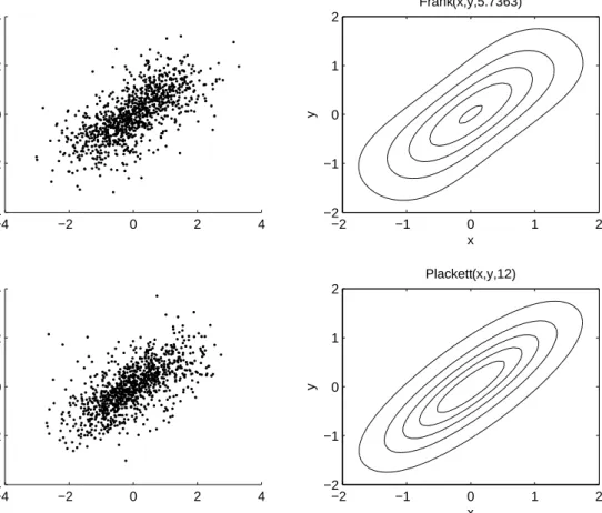
In figures 1-3 we present scatterplots and contour lines for some of the most popular copulas with standard normal margin and parameters corresponding to Kendall’s tau equal to 0.5. The difference in the dependence structure and the asymmetries for the Clayton and Gumbel copulas are quite easy to see.
−4 −2 0 2 4 −4 −2 0 2 4 x y Gumbel(x,y,2) −2 −1 0 1 2 −2 −1 0 1 2 −4 −2 0 2 4 −3 −2 −1 0 1 2 3 4 x y Gumbelrot(x,y,2) −2 −1 0 1 2 −2 −1 0 1 2
−4 −2 0 2 4 −4 −2 0 2 4 x y Clayton(x,y,2) −2 −1 0 1 2 −2 −1 0 1 2 −4 −2 0 2 4 −4 −3 −2 −1 0 1 2 3 x y Claytonrot(x,y,2) −2 −1 0 1 2 −2 −1 0 1 2
Figure 2: Illustration of the Clayton and survival Clayton copula
2.3
Simulation from a copula
A possible application of copula functions is the efficient simulation of an asset return dis-tribution in a more realistic way or, more generally, simulation from any disdis-tribution with dependent observations. By using the right copula, or even a mixture of two or more cop-ulas, and the corresponding parameters any dependence structure may be imposed. The simulated data offers itself to a variety of Monte Carlo methods.
Conditional sampling
The following algorithm is the most general one that can be used to simulate a sample from any copula. However, the method is not always the most efficient one, so more efficient
−4 −2 0 2 4 −4 −2 0 2 4 x y Frank(x,y,5.7363) −2 −1 0 1 2 −2 −1 0 1 2 −4 −2 0 2 4 −4 −2 0 2 4 x y Plackett(x,y,12) −2 −1 0 1 2 −2 −1 0 1 2
Figure 3: Illustration of the Frank and Plackett copula
ways will be discussed below. Whenever one of the algorithms described below is applicable it should be used. The marginal series obtained by the algorithm have the uniform (0,1) distribution, but as a result of Sklar’s theorem can be transformed into any distribution with-out changing the dependence structure using the method above. The following algorithm is known as theconditional distribution method. The conditional distribution can be obtained as follows.
C(v|u) =P[V ≤v|U =u] = ∂C(u, v)
∂u (12)
1. Generate two independent uniform (0,1) variates u and t;
3. The pair (u, v) has joint distribution function C.
Note that if the inverse of C cannot be found analytically, it has to be obtained using numerical root finding. Unfortunately, this makes the algorithm particularly slow.
Simulation from elliptical copulas
Let Ω denote the covariance matrix, which is positive definite, and let A be defined such that Ω =AAT. Then if Z=Z
1, ..., Zm i.i.d.∼ N(0,1) it follows that
µ+AZ∼Nm(µ,Ω).
This can be used to efficiently simulate random variates from a Gaussian copula using the Cholesky decomposition to impose the dependence on the independent random variables.
1. Find the Cholesky decomposition A of Ω.
2. Simulate 2 independent standard normal random variates z1 and z2.
3. Setx=Az.
4. Set u = φ(x1) and v =φ(x2), where φ
denotes the univariate standard normal cdf.
5. The pair (u,v) has the Gaussian copula as its distribution function.
In order to simulate a t-copula we use the relationship that if S has a chi-square distri-bution andZ is the same as above, then
X=dµ+ √
ν
√
SZ
has the multivariate t-distribution with ν degrees of freedom. The first three steps of the algorithm are the same as for the Gaussian copula. The remaining steps are:
4. Simulate a random variate s from X2
ν independent of z1 and z2.
5. Sety=√√ν
sx.
6. Set u = tν(y1) and v =tν(y2).
7. The pair (u,v) has the t-copula as its distribution function. Simulation from Archimedean copulas
results also find their application for testing the goodness-of-fit of copulas. Theorem 2.3.1Let C be an Archimedean copula generated by ϕ and let
KC(t) = VC({(u, v)∈[0,1]2|C(u, v)≤t}).
Then for any t in [0,1],
KC(t) =t− ϕ(t)
ϕ0
(t+). (13)
Corollary 2.3.2If (U, V)T has distribution function C, where C is an Archimedean copula
generated by ϕ, then the function KC is the distribution function of the random variable
C(U,V).
The theorem below allows for a direct implementation of the algorithm for simulating the copulas.
Theorem 2.3.3 Under the hypotheses of Corollary 2.3.2, the joint distribution function H(s,t) if the random variables S =ϕ(U)/[ϕ(U)+ϕ(V)]and T=C(U,V) is given by H(s,t)=sKC(t)
for all (s,t) in[0,1]2. Hence S and T are independent, and S is uniformly distributed on [0,1].
Now we are ready to present the algorithm:
1. Simulate two independent U(0,1) random variates s and q. 2. Set t = K−1
C (q), where KC is the distribution function of C(U,V). 3. Set u = ϕ[−1](sϕ(t)) and v = ϕ[−1]((1−s)ϕ(t)).
4. The desired pair is (u,v).
3
Estimation and model selection
When modeling the joint density of two random variables using copula functions, care needs to be taken as to how to correctly and efficiently estimate the parameters and how to discrim-inate between competing models. A number of methods exist for the estimation of copula functions and have been described in the literature. However, when it is best to use one of the methods is not always an easy issue. Tests of correct model specification of the marginals and the copula exist and some alternatives have been developed recently.
3.1
Estimation
There exist five methods of estimating copula models. The one step method or exact maxi-mum likelihood (EML) method estimates all parameters of the model at the same time. The second method is the two step estimator or the method of inference functions for margins (IFM), which first estimates the parameters of the marginals and with these parameters given estimates the copula function. The canonical maximum likelihood method (CML), or the semiparametric estimation, leave the marginal densities unspecified and uses the empirical probability integral transformin order to obtain the uniform marginals needed to estimate the copula parameters. The last two methods are nonparametric ways of estimating the copula. The first one is estimating the empirical copula directly from the data, leaving the whole specification nonparametric. The other is obtaining a nonparametric estimate for Kendall’s tau and using the relationship between Kendall’s tau and the copula parameter to get an estimate of the latter. This method is due to Genest and Rivest (1993) and is mainly suited for Archimedean copulas.
Exact maximum likelihood (EML)
Let θ ∈ Θ be the parameter vector to be estimated. This parameter vector can be split up into the parameters for the marginals and the copula function as follows θ = [ϕ0, γ0, δ0]0.
ϕ ∈ φ denotes the parameter(s) of f(x), γ ∈ Γ denotes the parameter(s) of g(y), and
δ∈∆ denotes the parameter(s) ofc(F(x), G(y)). Assume we observe a samplext and yt for
t = 1, ..., T. Consider the following representation of the joint density known as the copula decomposition of a joint distribution and the resulting log-likelihood function.
h(xt, yt;θ) =f(xt;ϕ)·g(yt;γ)·c(F(xt;ϕ), G(yt;γ);δ) LXY = T X t=1 ln(f(xt;ϕ)) + T X t=1 ln(g(yt;γ)) + T X t=1 ln(c(F(xt;ϕ), G(yt;γ);δ)) =LX(ϕ) +LY(γ) +LC(ϕ, γ, δ)
The ML estimator is then given by: ˆ
θ = arg maxLXY
This estimator is fully efficient as it attains the minimum asymptotic variance bound when the amount of data available for the two series is equal. However, it may be computationally difficult to obtain these estimates. Standard errors can be obtained in the usual way by the inverse of the Fisher information matrix.
The parametric two-step estimator (IFM)
This estimator makes use of the neat form of the copula decomposition of a joint distri-bution. In the first step the parameters ϕand γ of the marginal densities are estimated by MLE, i.e.
ˆ
ϕ= arg maxLX ˆ
γ = arg maxLY.
Using these estimates to transform the marginals into uniform (0,1) variables one can now estimate we can now estimate the copula parameter(s) δ by maximizing the copula density, i.e.
ˆ
δ = arg maxLC( ˆϕ,γ, δˆ ).
Joe and Xu (1996) showed that this estimator is consistent and asymptotically normal. The asymptotic covariance matrix ofT1/2(ˆθ−θ) is called the Godambe information matrix.
If we denote the vector of score functions of our model by ψθ(X, Y) then it is given by
V =D−1M(D−1)0, whereD=E[∂ψ
θ(X, Y)/∂θ] andM =E[ψθ(X, Y)ψθ(X, Y)0]. Note that this is just the standard covariance matrix for Z-estimators, see e.g. van der Vaart (1998). Joe and Xu (1996) suggest using the Jackknife method as an estimator for the covariance matrix and show its validity. If we denote the estimate of θ with the t’th row deleted from the data byθ(t), then the Jackknife estimator of T−1V is
T
X
t
(ˆθ(t)−θˆ)(ˆθ(t)−θˆ)0.
In case the sample is large one may delete the data block wise and the approach remains valid.
The IFM approach has the advantage of being computationally less demanding than the EML approach. Furthermore, estimating the margins in a first step allows to assess the goodness of fit of the margins separately from that of the copula. Another advantage of this estimator is that it allows the two series xt and yt to be of unequal length. W.l.g. assume that the amount of data available for X, Tx, is greater than the amount of data available for Y, Ty. Then the additional information on the random variable X can be used to find a better estimate of ϕ, which may lead to a better performance of the two-step estimator. Whether the use of this additional information offsets the loss of efficiency compared to the one-step estimator depends on the ratios Ty
Tx ≡ λy and Tc
Tx ≡ λc, where Tc is the number of observations available for the estimation of the copula, 0< λy <1 and 0< λc<1.
Patton (2006b) proposes a one-step adjustment of this estimator, that theoretically makes it fully efficient. However, in a Monte Carlo study the small sample properties of this adjusted estimator are shown to be rather poor. In contrast, the unadjusted estimator outperforms the EML estimator in the setup chosen.
The semi parametric two-step estimator (CML)
When the density of the marginal distributions are unknown this estimator gives the pos-sibility of leaving them unspecified. Bad estimation results due to miss specification of the marginals can be avoided. In the first step the series of interest are transformed into uni-form variates using the empirical probability integral transuni-form. The empirical distribution function is defined as ˆ F(·) = 1 T T X t=1 1{Xt≤·}, (14)
where 1{Xt≤·} is the indicator function. The copula parameter δ can the be estimated by maximizing the log-likelihood function of the copula density using the transformed variables given by LC(δ) = T X t=1 ln(c( ˆF(xt),Gˆ(yt))) = T X t=1 ln(c( ˆut,vˆt). (15) The semi parametric estimator then is
ˆ
δ= arg maxLC(δ).
Consistency and asymptotic normality of the CML estimator were shown by Genest et al. (1995) for the i.i.d. case and by Chen and Fan (2006) for estimating copula based time series models. Chen and Fan (2005) showed that this estimator also converges to the pseudo true parameter in case the copula is misspecified (which in most practical situations is very likely), so that the estimated model is closest to the data generating process in terms of the Kullback-Leibler divergence.
Estimators for the covariance matrix are described by the authors for the various cases. For a clear step by step procedure for the i.i.d. case we refer to Genest and Favre (2005).
The nonparametric estimator
Unlike the methods described above this method does not rely on any parametric speci-fication of the copula function. Theempirical copula is the functionCn given by
Cn(
i T,
j T) =
number of pairs (xt, yt) in the sample such that xt≤xi and yt ≤yj
T ,
for i, j = 1, ..., T. The empirical copula can be used to calculate population versions of the concordance measure described above. For more details on that see Nelson (1999). Addi-tionally, they find their use in nonparametric tests for independence and for goodness of fit test of the copula specification. Note that Fermanian and Scaillet (2003) also propose a kernel estimator for copulas.
The nonparametric estimator by Genest and Rivest
An advantage of this approach is that the marginal distributions do not need to be speci-fied. If we let c denote the number of concordant pairs in the sample and d the number of discordant pairs in the sample, then the sample version of Kendall’s tau is given by
ˆ
τ = c−d
c+d. (16)
Using this estimate and the relationship between the copula parameter and Kendall’s tau the nonparametric estimate can be obtained easily if a closed form expression for this relationship exists. In case a closed form expression does not exists one can still estimate the copula parameter by using the general form of Kendall’s tau for Archimedean copulas. This takes the form τC = 1 + 4 Z 1 0 ϕ(t) ϕ0 (t)dt
and might be solved using a computer program like Mathematica or Maple. An obvious drawback of this estimator is that it only applies to the limited number of one parameter models. When it is available one may compare the parameter estimate of the copula model to the estimate obtained by a MLE for a first check of its goodness-of-fit. When the two estimates are close to each other one has an indication of a reasonable fit.
3.2
Model selection
Once one or more estimates of a certain copula have been obtained a very important issue is how to compare the competing models. The first thing to be done is to assess the goodness-of-fit of the marginal distribution. Both the i.i.d.’ness and the correct specification of the
distribution need to be tested. For testing the i.i.d.’ness we refer to Diebold, et al.(1997) who proposed a simple procedure for this task. The specification of the distribution can be tested by testing the transformed series for uniformity. This can be done by using the well known Kolmogorov-Smirnov test or a Chi-square test.
A huge number of tests have been proposed for testing the copula specification. Examples are Chen et al. (2004), Chen and Fan (2005), Genest et al. (2006) and Fermanian (2003). However, none of these tests has proven to be superior and quite some research remains to be done in this field. Besides the numerous goodness-of-fit tests there are a few model selection criteria, which allow to rank the copulas according to their fit in some way. The most widely used criterium is the Akaike information criterion. It is defined as
AIC = 2(negative log-likelihood) + 2k
wherek is the number of parameters in the model. The model with the lowest AIC should be considered as the best fitting one.
Graphical methods
The first step we propose in the model selection process is a visual inspection of the scatter-plot of the data. Some dependence structures may already be identified such as dependence in one of the tails. However, there are more formal ways of assessing the goodness-of-fit of your model by visual means. Consider the conditional distribution function(d.f.) ofY given
X. It is given by
HY|X(x, y) =C1(F(x), G(y))
where C1(u, v) = ∂u∂ C(u, v). The conditional d.f. is U(0,1) distributed, if the joint density
is well specified. Therefore a QQ-plot of the conditional d.f. using the estimated parameter and the observed datax and y against uniform quantiles should yield a straight line.
A similar method makes use of Theorem 2.3.1 and Corollary 2.3.2, which state that the distribution function of the copula can be represented in the following way:
KC(t) =P[C(U, V)≤t] = t−
ϕ(t)
ϕ0 (t+)
Therefore KC(C(F(X), G(Y)) should be uniformly distributed, so in a similar fashion as above the QQ-Plot can be constructed and can be compared to a straight line.
A third method, which was proposed by Genest and Rivest(1993), relies on two estimates for the distribution function of the copulaKC. One is a parametric estimate obtained by MLE, the other is the empirical copula, which is determined by the method described in section
3.1. A QQ-Plot of these two distribution function should help determine the best fitting copula. For a good exposition of this method, possible drawback, and some applications the reader is referred to Matteis (2001). Note that again we can also look at the histogram of the d.f. of interest and compare it to the histogram of aU(0,1) variate. The histogram should be close to a horizontal line under a good specification.
Tests based on the graphical methods
The idea that both the conditional d.f. and the d.f. of the copula should follow a U(0,1) distribution under a correct specification of the copula can also be used to conduct formal tests. Matteis (2001) (among others) proposes to apply the Kolmogorov-Smirnov (K-S) test and the Chi-square test to check the null hypothesis of a U(0,1) distribution.3 We suggest
additionally using the Jarque-Bera test after transforming the data through the inverse CDF of the normal distribution.
As mentioned above there are many more tests available for testing the goodness-of-fit of the copula specification. However, we postpone a systematic comparison.
4
Simulation study
So far the different estimators and some simple model selection tests for copula functions have been introduced. However, small sample performance of both the different estimators and the testing procedures are not always obvious. In order have a better idea on how to properly model data using copulas Monte Carlo experiments will be performed. The setup of the simulations are supposed to resemble decisions that have to be made by a researcher working on practical issues. This could include issues like which estimation technique to use, which copula functions to consider to describe certain dependence structures, small sample power of a certain test, behavior of competing tests under misspecification, etc. In the copula literature Monte Carlo studies are frequently performed, but often attention is only paid to testing the power of a certain test under a very limited number of data generating processes, as a general setting is not always possible. A problem is that most competing copula models are non-nested. Therefore, a lot of questions remain open and it is easy to set up interesting studies. Here we will consider two different simulation studies. In the first the properties of the different estimation techniques are compared, both when the density of the marginals is known and when it is misspecified. In the second an attempt is made to compare the methods for model selection for competing copula models we presented above.
3For the third method he uses only the K-S test, as it must be checked whether two distributions are
4.1
Comparison of the estimators
In this section we want to take a closer look at the properties of the estimator that have been suggested in the literature. Theoretically their properties have been well studied and we expect to confirm the theoretical findings. We consider the following estimators: EML, IFM, CML and the nonparametric estimator based on Kendall’s tau, which we shall call method of moments (MM) here. The data generating process is a rather simple one. Data is simulated from a Clayton copula with its parameter corresponding to Kendall’s tau equal to 0.2, 0.4, 0.6 and 0.8. As marginal distributions we took t-distributions with 5 and 6 degrees of freedom for theX and Y series, respectively. Formally, we have
(u, v)∼CδClayton X=t−1(u; 5)
Y =t−1(v; 6).
The sample sizes we look at are 100, 250, 500 and 1000 observations. All simulations will be replicated 1000 times. We only focus on the estimation of the copula parameter, although one has to keep in mind that for the EML and IFM estimators additionally the degrees of freedom parameter needs to be estimated. We use these two estimator both in the situation when the marginals are known to follow a t-distribution and when they are wrongly speci-fied, which is a situation that is highly relevant in practice. In particular, normal marginals are estimated in the misspecified case. For the CML and the MM estimators, of course, the marginals remain unspecified. Theoretically the EML estimator is the most efficient one, fol-lowed by the IFM estimator and the CML estimator, but it remains to be seen whether this also holds in our simulation setup and how large the gain in efficiency is. Another interesting issue is how the CML and MM estimators compare to the misspecified estimators, because it can provide a guideline as to which estimator to use whenever one is not sure about the specification of the marginal distributions.
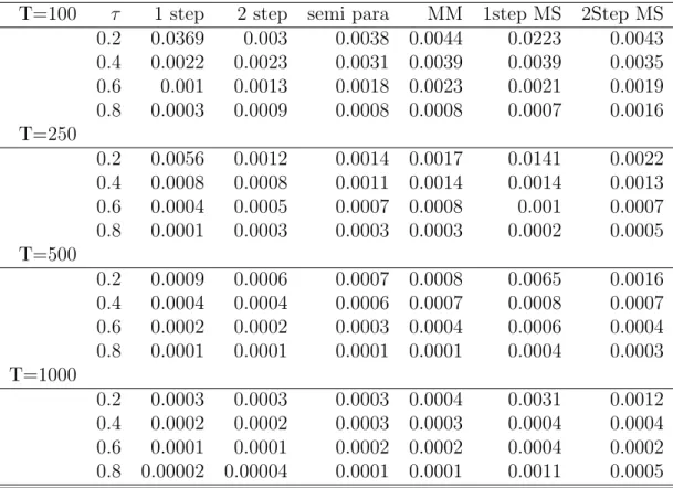
Table 1 reports the Mean Square Errors (MSE) of the estimates for Kendall’s tau corre-sponding to the estimated copula parameter and its true value. We decided to compute the MSE for Kendall’s tau and not for the copula parameter itself, because that allows compar-ison of the efficiency over different degrees of dependence. Overall the EML estimator is in fact superior to the others, but for weak dependence structures the IFM method is actually better and the difference between the two is rather small. For correctly specified models the MM estimator is the worst. The CML estimator is, as expected, not as efficient as the fully parametric methods. Only for tau equal to 0.2 andT less than 1000 does it outperform the EML method. When the marginals are misspecified the IFM estimator is clearly superior to the EML estimator. However, it is almost always worse than the semi-parametric estimator. Thus, whenever one fears that the marginals are misspecified we recommend using the CML
Table 1: Mean Square Errors for different estimators
T=100 τ 1 step 2 step semi para MM 1step MS 2Step MS
0.2 0.0369 0.003 0.0038 0.0044 0.0223 0.0043 0.4 0.0022 0.0023 0.0031 0.0039 0.0039 0.0035 0.6 0.001 0.0013 0.0018 0.0023 0.0021 0.0019 0.8 0.0003 0.0009 0.0008 0.0008 0.0007 0.0016 T=250 0.2 0.0056 0.0012 0.0014 0.0017 0.0141 0.0022 0.4 0.0008 0.0008 0.0011 0.0014 0.0014 0.0013 0.6 0.0004 0.0005 0.0007 0.0008 0.001 0.0007 0.8 0.0001 0.0003 0.0003 0.0003 0.0002 0.0005 T=500 0.2 0.0009 0.0006 0.0007 0.0008 0.0065 0.0016 0.4 0.0004 0.0004 0.0006 0.0007 0.0008 0.0007 0.6 0.0002 0.0002 0.0003 0.0004 0.0006 0.0004 0.8 0.0001 0.0001 0.0001 0.0001 0.0004 0.0003 T=1000 0.2 0.0003 0.0003 0.0003 0.0004 0.0031 0.0012 0.4 0.0002 0.0002 0.0003 0.0003 0.0004 0.0004 0.6 0.0001 0.0001 0.0002 0.0002 0.0004 0.0002 0.8 0.00002 0.00004 0.0001 0.0001 0.0011 0.0005
Note: The table reports the MSE from the implied Kendall’s tau to the true one. Data is generated from a Clayton copula with Student t margins. EML MS and IFM MS refer to the estimator when the margins are assumed to be normally distributed.
method. In case a fully parametric estimate is needed (e.g. because the behavior of some test statistic is not known for a semi-parametric estimator) we recommend using the IFM estimator. Note that as the sample size and the degree of dependence increase the MSE’s greatly decrease.
4.2
Model selection
A typical problem that arises when fitting copulas to data is how to decide for the best fitting model. A large number of methods has been proposed for that end. Here we compare the ones we proposed earlier, namely the AIC and three tests for checking whether the conditional
Table 2: Model selection by AIC when the true model is the Gumbel copula
T=100 τ Gumbel rot. Gumbel Clayton rot. Clayton Frank Plackett Normal 0.2 0.333 0.037 0.015 0.373 0.053 0.077 0.112 0.4 0.588 0.009 0 0.227 0.023 0.044 0.109 0.6 0.806 0 0 0.09 0.019 0.019 0.066 T=250 0.2 0.54 0.008 0 0.277 0.031 0.056 0.088 0.4 0.844 0 0 0.113 0.004 0.008 0.031 0.6 0.978 0 0 0.016 0 0 0.006 T=500 0.2 0.731 0 0 0.205 0.013 0.012 0.039 0.4 0.95 0 0 0.046 0 0.001 0.003 0.6 0.998 0 0 0.001 0 0 0.001 T=1000 0.2 0.856 0.001 0 0.125 0.001 0.002 0.015 0.4 0.99 0 0 0.01 0 0 0 0.6 1 0 0 0 0 0 0
copula is distributed uniformly, which are the K-S test, the Chi-square4 test and the
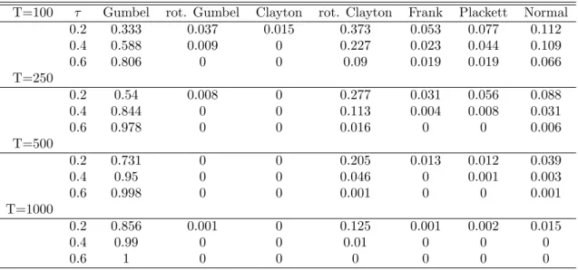
Jarque-Bera test. In our first simulation we sample data from three different copulas, the Gumbel, Clayton and Frank copulas withU(0,1) marginals and parameters corresponding to Kendall’s tau equal to 0.2, 0.4 and 0.6 and sample sizes of 100, 250, 500 and 1000 observations. Then we estimate the following copulas: Gumbel, survival Gumbel, Clayton, survival Clayton, Frank, Plackett and Normal copula, which are the most popular one-parameter copulas in the literature.5 Tables 2-4 report the fraction of times each candidate model is chosen when
using a selection rule the always decides for the model with the smallest AIC. This model selection procedure becomes more powerful with stronger dependence and larger samples sizes. In most of the cases when the true model is not selected the model with the lowest AIC is one with similar dependence structure. For example both the Gumbel and the rotated Clayton copula are characterized by upper tail dependence and one can see that when the data is generated from a Gumbel copula the rotated Clayton copula is selected quite often. Altogether one can say that the AIC is a good criterion for finding the best fitting copula. However, for weak dependence its performance is not entirely satisfactory. The good news is that when it does not find the correct model it will usually chose one that is close to it.
4For the Chi-square test we use 15, 20, 30 and 50 classes for 100, 250, 500 and 1000 observations,
respectively.
Table 3: Model selection by AIC when the true model is the Clayton copula
T=100 τ Gumbel rot. Gumbel Clayton rot. Clayton Frank Plackett Normal 0.2 0.01 0.192 0.647 0.001 0.041 0.033 0.076 0.4 0 0.153 0.829 0 0.01 0.001 0.007 0.6 0 0.07 0.93 0 0 0 0 T=250 0.2 0.001 0.205 0.735 0 0.019 0.013 0.027 0.4 0 0.085 0.915 0 0 0 0 0.6 0 0.008 0.992 0 0 0 0 T=500 0.2 0 0.185 0.808 0 0 0.002 0.005 0.4 0 0.021 0.979 0 0 0 0 0.6 0 0.002 0.998 0 0 0 0 T=1000 0.2 0 0.092 0.908 0 0 0 0 0.4 0 0.002 0.998 0 0 0 0 0.6 0 0 1 0 0 0 0
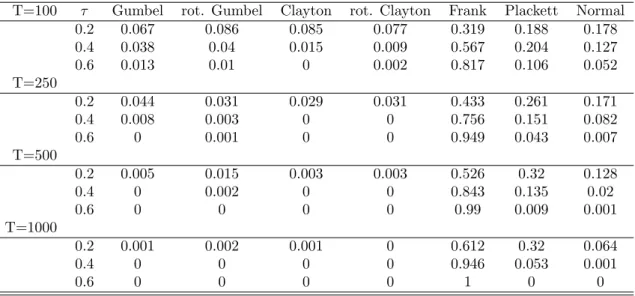
Table 4: Model selection by AIC when the true model is the Frank copula
T=100 τ Gumbel rot. Gumbel Clayton rot. Clayton Frank Plackett Normal 0.2 0.067 0.086 0.085 0.077 0.319 0.188 0.178 0.4 0.038 0.04 0.015 0.009 0.567 0.204 0.127 0.6 0.013 0.01 0 0.002 0.817 0.106 0.052 T=250 0.2 0.044 0.031 0.029 0.031 0.433 0.261 0.171 0.4 0.008 0.003 0 0 0.756 0.151 0.082 0.6 0 0.001 0 0 0.949 0.043 0.007 T=500 0.2 0.005 0.015 0.003 0.003 0.526 0.32 0.128 0.4 0 0.002 0 0 0.843 0.135 0.02 0.6 0 0 0 0 0.99 0.009 0.001 T=1000 0.2 0.001 0.002 0.001 0 0.612 0.32 0.064 0.4 0 0 0 0 0.946 0.053 0.001 0.6 0 0 0 0 1 0 0
In order to get an idea about the size and the power under different alternatives of the three goodness-of-fit tests we consider the problem of testing whether data has been generated by a Gaussian copula. To this end we draw random observations from the Gaussian copula in order check the size of the tests and from two alternatives, namely the t-copula with 4 degrees of freedom and the Clayton copula. The t-copula is chosen to see the behavior of the test when the alternative as also symmetric, but has fatter tails than then null. The Clayton copula, on the other hand, has an asymmetric dependence structure and we expect the tests to have higher power against this alternative.
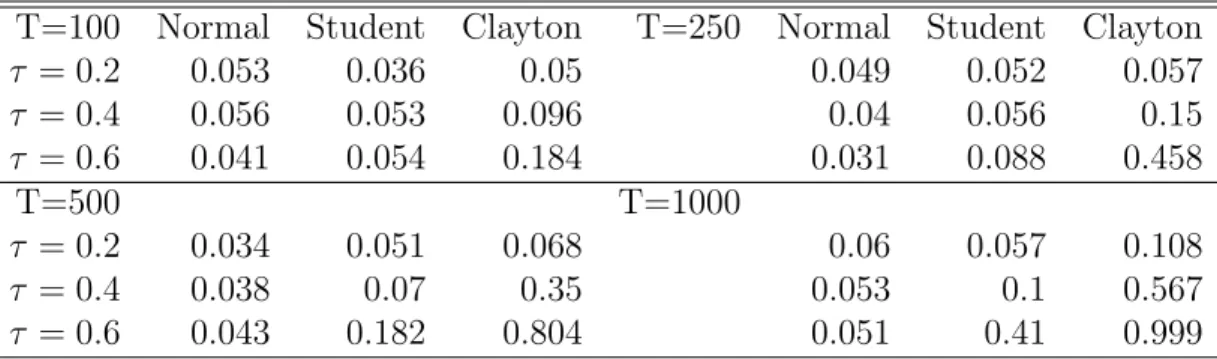
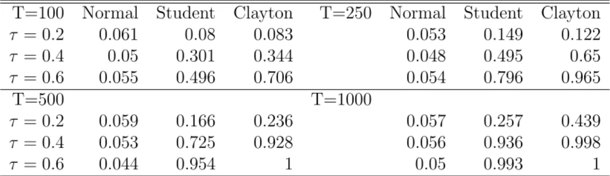
In tables 5-7 the rejection frequencies at a level of 5% for the three mentioned tests are given. First note that all 3 tests have a higher power against the Clayton copula as the alternative, than against the t-copula. In terms of size the K-S test performs quite well. It seems to be slightly undersized. Its power, however, is only acceptable for strong dependence structures and large samples. The Chi-square test is clearly oversized, but its power a lot higher than for the K-S test. Finally, the Jarque-Bera test has both good size properties and it is superior to the other two tests in terms of power. Thus the Jarque-Bera test is the most recommendable test of the three. This may be due to the fact that is able to detect skewness and excess kurtosis, which in terms of copulas means it is able to detect if a model insufficiently captures asymmetric dependence or fat tails. Still one can see that the performance of the tests is not acceptable for weak dependence structures even when the sample is large. Thus we conclude that these tests are not very useful in small samples and for weak dependence. They are powerful only in situations when model selection using the AIC works extremely well. The K-S test is the weakest of the three and it should be interpreted with care. The Chi-square and especially the Jarque-Bera test can be useful for complementing model selection by the AIC. Furthermore, formal testing is necessary, since one cannot be sure that the true model is among the ones selected for estimation. Thus, even when a model clearly outperforms its competitors in terms of AIC none of the copulas estimated may have a satisfactory fit.
Table 5: Rejection frequencies for the KS-test
T=100 Normal Student Clayton T=250 Normal Student Clayton
τ = 0.2 0.053 0.036 0.05 0.049 0.052 0.057 τ = 0.4 0.056 0.053 0.096 0.04 0.056 0.15 τ = 0.6 0.041 0.054 0.184 0.031 0.088 0.458 T=500 T=1000 τ = 0.2 0.034 0.051 0.068 0.06 0.057 0.108 τ = 0.4 0.038 0.07 0.35 0.053 0.1 0.567 τ = 0.6 0.043 0.182 0.804 0.051 0.41 0.999
Note: Data is generated from a Gaussian copula, a t-copula with 4 degrees of freedom and a Clayton copula withU(0,1) margins. The table reports the frequency of rejection of tests of uniformity of the conditional gaussian copulaCGaussian(u|v).
Table 6: Rejection frequencies for the Chi-square test
T=100 Normal Student Clayton T=250 Normal Student Clayton
τ = 0.2 0.1 0.091 0.093 0.073 0.1 0.106 τ = 0.4 0.079 0.084 0.162 0.077 0.099 0.301 τ = 0.6 0.058 0.108 0.354 0.078 0.139 0.74 T=500 T=1000 τ = 0.2 0.083 0.076 0.117 0.077 0.069 0.139 τ = 0.4 0.071 0.105 0.517 0.065 0.135 0.772 τ = 0.6 0.076 0.237 0.959 0.081 0.414 1
Note: Data is generated from a Gaussian copula, a t-copula with 4 degrees of freedom and a Clayton copula withU(0,1) margins. The table reports the frequency of rejection of tests of uniformity of the conditional gaussian copulaCGaussian(u|v).
Table 7: Rejection frequencies for the JB-test
T=100 Normal Student Clayton T=250 Normal Student Clayton
τ = 0.2 0.061 0.08 0.083 0.053 0.149 0.122 τ = 0.4 0.05 0.301 0.344 0.048 0.495 0.65 τ = 0.6 0.055 0.496 0.706 0.054 0.796 0.965 T=500 T=1000 τ = 0.2 0.059 0.166 0.236 0.057 0.257 0.439 τ = 0.4 0.053 0.725 0.928 0.056 0.936 0.998 τ = 0.6 0.044 0.954 1 0.05 0.993 1
Note: Data is generated from a Gaussian copula, a t-copula with 4 degrees of freedom and a Clayton copula withU(0,1) margins. The table reports the frequency of rejection of tests of uniformity of the conditional gaussian copulaCGaussian(u|v).
5
Modeling exchange rate dependence
Now that we have introduced copula functions, the different ways of estimating them for a given data set and some model specification tests, including an analysis of their finite sam-ple properties, we are ready to present their use in practice. We use copulas to model the dependence between pairs of Latin American exchange rates against the Euro. In particular we consider daily exchange rate returns from 01/01/2001 until 30/11/2006, which amounts to 1485 observations for each series, for the following countries: Brazil, Chile, Columbia, Mexico and Peru.6
All the results on estimation and model selection require i.i.d. U(0,1) observations. This requires a first estimation step to filter out mean dynamics and heteroscedasticity. Autocor-relation or an incorrect specification of the marginal distribution can influence the estimation of the copula parameters. The first step in modeling the data is to model the marginal dis-tribution of each series individually in order to transform them into i.i.d. U(0,1) series. To this end we start by fitting ARMA models to each series and then fitting GARCH models to their residuals. The mean dynamics where captured well by only an intercept for all series except Mexico. In that case a simple AR(1) model provided a good fit for the data. The best fit for the conditional variance was a t-GARCH(1,1) for all series. The standardized resid-uals where fit to a Student t-distribution using maximum likelihood estimation (MLE) and transformed into U(0,1) variables using the CDF of the t-distribution and the estimated
6The data have been taken from the internet page of the PACIFIC Exchange Rate Service provided by
degrees of freedom parameter. The uniformity is tested using the tests also proposed for the goodness-of-fit tests for copulas, the K-S test, the Chi-square test and the Jarque-Bera test. Non of the series passed all three tests, so the uniformity assumption is questionable. Therefore we modeled the standardized residuals with the skewed t-distribution introduced by Hansen (1994). The p-values of the goodness-of-fit a given in table 8.7 All series fit
the skewed t-distribution quite well so we can continue working with the transformed series. Note that the skewness parameters were quite small (below 0.1 in absolute values) for all series.
The second step is actually estimating a number of copulas and deciding which is the best Table 8: Goodness-of-fit tests for marginal distributions
Bra Chi Col Mex Peru
KS 0.6361 0.5455 0.8814 0.5246 0.5465 Chi2 0.2486 0.5941 0.3247 0.8275 0.0829 JB 0.9044 0.8643 0.9424 0.979 0.9237
Note: The series have been fit to a skewed t-distribution and were transformed by the skewed t CDF.
fitting one. The estimation is done using the IFM method, since we have already modeled the marginals and we found that IFM estimator behaves quite well compared to the one step estimator. An argument for using the EML technique is that it is easier to get the standard errors, but we are not interested in testing any hypothesis about the parameters. We also estimated all the models with the semi-parametric estimator, but the results were very close to the fully parametric approach, so we report only the outcomes for the latter estimator. To get an idea of the degree of dependence between the series we the Kendall’s tau matrix is given in table 9. It ranges from 0.36 for the pair Brazil-Columbia until 0.57 for Peru-Mexico. The copulas we estimate are the following: Gumbel, survival Gumbel, Clayton, survival Clayton, Frank, Plackett, Normal, Student, Joe-Clayton(JC), symmetrized JC, BB1, mixture Clayton-Gumbel, mixture Clayton-Frank, mixture Frank, mixture Gumbel-survival Gumbel, mixture Clayton-Gumbel-survival Clayton and mixture JC-Frank. All copulas are estimated and the models were ranked according to the AIC. Then the Jarque-Bera test on the conditional copula is performed (after transforming the series with the inverse Gaussian CDF as before). The test was performed both for the conditional copula U given V and V given U, so the derivative of the copula distribution function with respect to each of its arguments. The highest ranked model that passed the Jarque-Bera test in both directions is
Table 9: Kendall’s tau matrix between the GARCH residuals
bra chi col mex peru
bra 1 0.4513 0.3602 0.4346 0.3649
chi 0.4513 1 0.4299 0.5129 0.4727
col 0.3602 0.4299 1 0.5018 0.5721
mex 0.4346 0.5129 0.5018 1 0.5785
peru 0.3649 0.4727 0.5721 0.5785 1
considered the best fitting one. In some cases, however, models were very close to each other in terms of the AIC, so deciding for the best fitting one is a rather hard task. More refined model selection techniques may be necessary in this case. In such situations we simply report more than one model. Overall there are three dominant copulas, the Student copula, the Joe-Clayton-Frank mixture and the mixture Gumbel-survival Gumbel. Furthermore, it is apparent that all pairs of exchange rates exhibit tail dependence in both tails. Models that do not allow for dependence in both tails are not among the best fitting ones. We make the same observation as Junker et al. (2005) that a one parameter copula is not able to provide a reasonable fit for financial data.
For the pairs Brazil-Chile, Brazil-Columbia and Brazil-Mexico we observe an asymmetric de-pendence structure with more upper tail dede-pendence than lower tail dede-pendence. This means that when these currencies depreciate against the Euro they tend to be more dependent that when they appreciate. However, for the pair Brazil-Mexico the evidence is not that strong and dependence may actually be symmetric. The pairs Chile-Columbia, Columbia-Peru also have an asymmetric dependence structure, but they have more lower tail dependence than upper tail dependence. For the rest of the pair we can conclude that dependence is rather symmetric. Only for the pair Columbia-Mexico is there some evidence for excess upper tail dependence. Our findings are in line with the findings of Patton (2006a,b) who finds asymmetric dependence for the Euro/German Mark and the Yen against the dollar. Note that just as found in Patton (2006a) exchange rate dependence may be varying over time and should therefore be modeled using conditional copula models. We leave this for future research.
Table 10: Estimation results
Countries Model δ1 δ2 α λU λL AIC
bra-chi
JC-Frank 1.6609; 0.5369 6.2095 0.5173 0.2494 0.1423 -787.169 Student 0.6411 12.1674 - 0.1132 0.1132 -782.364 bra-col
Gumbel- rot. Gumbel 1.5091 1.655 0.6843 0.2854 0.1515 -497.262 Clayton-Gumbel 1.3378 1.5201 0.2182 0.3301 0.1299 -495.439 Gumbel-Frank 1.4721 4.6115 0.6315 0.2518 0 -495.059 bra-mex JC-Frank 1.6302; 0.5742 5.4081 0.4498 0.2115 0.1345 -718.688 Student 0.6214 10.1643 - 0.1343 0.1343 -716.062 bra-peru Student 0.5344 7.5576 - 0.1433 0.1433 -502.37 Gumbel- rot. Gumbel 1.4132 1.8116 0.5623 0.2063 0.2337 -499.56 chi-col
Gumbel- rot. Gumbel 1.4722 2.1164 0.4516 0.18 0.3359 -758.907 chi-mex Student 0.719 14.1568 - 0.1361 0.1361 -1080.69 chi-peru Student 0.6763 5.1767 - 0.3156 0.3156 -943.031 col-mex JC-Frank 1.9722; 1.2787 5.4311 0.4904 0.2839 0.2852 -1002.99 Gumbel- rot. Gumbel 1.8917 2.102 0.5009 0.2793 0.3041 -1002.41 Clayton-Gumbel 2.4352 1.9038 0.3166 0.3832 0.2382 -999.295 col-peru
Gumbel- rot. Gumbel 1.6847 3.1345 0.3706 0.182 0.4736 -1439.48 mex-peru
Student 0.781 12.9949 - 0.2107 0.2107 -1392.82
Note: Estimation results for the best fitting copula models obtained by the IFM method for standardized GARCH residuals. In case of mixturesδ1is the estimate of the first model (two parameters in the JC-Frank
copula),δ2 is the estimate of the second model andαis the mixing parameter.
6
Conclusion
In this paper we introduced copula functions in a formal mathematical manner. We estab-lished some important links between copulas and some common measures of dependence, after presenting the relevant dependence concepts, in order to enable the reader to interpret these measures in a correct way. The introduction of the most commonly used examples and families of copulas, together with the different estimators and some goodness-of-fit tests,
gave us all the tools necessary to model a data set. However, the theory is not able to give any guidelines as to which copula functions to consider, which estimator to use or how to discriminate between competing models. Providing some guidelines to these issues turned out to be the main point of this work. With the help of Monte Carlo simulations we can recommend the use of the CML estimator whenever a fully parametric model is not needed and when one runs the danger of working with misspecified marginal distributions. When one is confident about the marginal distributions chosen, however, the IFM estimator is su-perior to the CML method in terms of mean-square-errors and it is extremely close to the EML estimator in terms of efficiency. We also gained some insight into the performance of different model selection criteria. The Akaike information criterion should be considered first when looking for the copula that most likely can capture the true dependence present in the data. The tests based on the conditional distribution function performed reasonable only for large samples and strong dependence. All three tests considered perform well in terms of size, but only the Jarque-Bera test, which had not been suggested in the literature for testing copula models until now, showed sufficient power to be recommended for empirical applications.
We used the techniques introduced to model the joint distribution of Latin American ex-change rate returns against the Euro by fitting a copula to the standardized residuals of an ARMA-GARCH model. We found evidence of asymmetric dependence, both excess upper and lower tail dependence, as well as symmetric joint movements in the data analyzed. We can conclude that copula models are, and will be, a very useful tool in econometrics for simulation, density forecasting and for analyzing nonlinear dependence. The simulation algorithms offer themselves as a tool for realistically simulating asset returns, which may be used for pricing exotic options or credit risk derivatives by simulation methods. The ability of copulas to model the complete joint distribution of a variable of interest turns out to be useful when analyzing risk for a set of variables. A classical example is the Value-at-Risk of a portfolio using copula based dependence measure instead of Pearson’s correlation coefficient. More copula based models in finance and risk management have arisen and can be expected to arise in the future. Furthermore, copulas can be used to model nonlinear dependencies between any type of economic variables. The existence of time varying copulas increases the possibilities for research. Even though applications outside financial econometrics are rare, one can expect the development of such models in the near future. Additional theoretic research needs to be conducted regarding model selection tests and the modeling of higher dimensional copulas. Once they become a more common tool, higher dimensional copulas will most probably be used in many empirical applications.