Dissertations
Summer 8-2008
Knowledge-Based Analysis of Genomic Expression Data by Using
Knowledge-Based Analysis of Genomic Expression Data by Using
Different Machine Learning Algorithms for the Purpose of
Different Machine Learning Algorithms for the Purpose of
Diagnostic, Prognostic or Therapeutic Application
Diagnostic, Prognostic or Therapeutic Application
Venkata Jagan Mohan ThodimaUniversity of Southern Mississippi
Follow this and additional works at: https://aquila.usm.edu/dissertations
Part of the Bioinformatics Commons, and the Biology Commons
Recommended Citation Recommended Citation
Thodima, Venkata Jagan Mohan, "Knowledge-Based Analysis of Genomic Expression Data by Using Different Machine Learning Algorithms for the Purpose of Diagnostic, Prognostic or Therapeutic Application" (2008). Dissertations. 1164.
https://aquila.usm.edu/dissertations/1164
This Dissertation is brought to you for free and open access by The Aquila Digital Community. It has been accepted for inclusion in Dissertations by an authorized administrator of The Aquila Digital Community. For more
NOTE TO USERS
Page(s) not included in the original manuscript and are unavailable from the author or university. The manuscript
was scanned as received.
The University of Southern Mississippi
KNOWLEDGE-BASED ANALYSIS OF GENOMIC EXPRESSION DATA BY USING
DIFFERENT MACHINE LEARNING ALGORITHMS FOR THE PURPOSE OF
DIAGNOSTIC, PROGNOSTIC OR THERAPEUTIC APPLICATION
by
Venkata Jagan Mohan Thodima
A Dissertation
Submitted to the Graduate Studies Office of The University of Southern Mississippi in Partial Fulfillment of the Requirements
for the Degree of Doctor of Philosophy
Approved
KNOWLEDGE-BASED ANALYSIS OF GENOMIC EXPRESSION DATA BY USING
DIFFERENT MACHINE LEARNING ALGORITHMS FOR THE PURPOSE OF
DIAGNOSTIC, PROGNOSTIC OR THERAPEUTIC APPLICATION
by
Venkata Jagan Mohan Thodima
A Dissertation
Submitted to the Graduate Studies Office of The University of Southern Mississippi in Partial Fulfillment of the Requirements for the Degree of Doctor of Philosophy
ABSTRACT
KNOWLEDGE-BASED ANALYSIS OF GENOMIC EXPRESSION DATA BY USING
DIFFERENT MACHINE LEARNING ALGORITHMS FOR THE PURPOSE OF
DIAGNOSTIC, PROGNOSTIC OR THERAPEUTIC APPLICATION
by Venkata J. Thodima
August 2008
With more and more biological information generated, the most pressing task of
bioinformatics has become to analyze and interpret various types of data, including
nucleotide and amino acid sequences, protein structures, gene expression profiling and so
on. In this dissertation, we apply the data mining techniques of feature generation, feature
selection, and feature integration with learning algorithms to tackle the problems of
disease phenotype classification, clinical outcome and patient survival prediction from
gene expression profiles.
We analyzed the effect of batch noise in microarray data on the performance of
classification. Batchmatch, a batch adjusting algorithm based on double scaling method is
advantageous over Combat, another batch correcting algorithm based on the empirical
bayes frame work. In order to identify genes associated with disease phenotype
classification or patient survival prediction from gene expression data, we compared and
analyzed the performance of five feature selection algorithms. Our observations from
these studies indicated that Gainratio algorithm performs better and more consistently
over the other algorithms studied.
In the aspect of classification algorithms, no single algorithm is absolutely superior to all
others, though SVM achieved fairly good results in most endpoints. Naive bayes
algorithm also performed well in some endpoints. Overall, from the total 65 models we
reported (5 top models for 13 end points) SVM and SMO (a variant of SVM) dominate
mostly, also the linear kernel performed well over RBF in our binary classifications.
DEDICATED TO
Deng, for his encouragement, patience and prompt help. Dr. Deng always provides me
complete freedom to explore and work on the research topics that I have interests in.
Although it was difficult for me to make quick progress at the beginning, I must
appreciate the wisdom of his supervision when I started to think for myself and become
relatively independent.
I would like to also thank the members of my dissertation committee, Dr.
Mohamed Elasri, Dr. Joe Zhang, Dr. Mac Alford and Dr. Jonathan Sun for their advice
and support throughout the duration of this project.
I would like to thank the participating members and working groups of
Microarray Quality Control (MAQC-II) consortium for their discussions and advice
during this collaborative project. I would especially like to thank Dr. Leming Shi,
principal investigator in NCTR, FDA and also the coordinator of this MAQC project, for
giving me the opportunity to participate in this project. I would also thank to the
Mississippi Functional Genomics Network (MFGN) for their support during this project.
I would like to thank to my colleagues Arun Rawat and Satish Pasula for their
efforts in reading the draft copy and suggesting clarifications, and my other lab members,
Dr. Mehdi Pirooznia, Tanwir Habib, Dr. Puneet Bandi, Kuan Yang and Ying Li for their
help during this project.
I could not have finished my dissertation work without the strong support from
my family. Special thanks must go to my parents and brother; together with them is my
wife, Harini, who is always there to provide me her support through both the highs and lows of my time.
DEDICATION v
ACKNOWLEDGEMENTS vi
LIST OF ILLUSTRATIONS x
LIST OF TABLES xii
CHAPTER
I. INTRODUCTION AND BACKGROUND 1
Motivation 1
Microarray Quality Control (MAQC) Consortium 4
Overview of the Project MAQC-I Findings Objectives of MAQC-II Design of MAQC-II
Supervised Learning and Classification Algorithms 12
Gene Expression Data Representation for Classification Results Evaluation and Error Estimation
Error Estimation Methods Classification Algorithms
Feature Selection Algorithm 27
Categorization of Feature Selection Algorithms Feature Selection Algorithms
Chapter Summary 34
II. MATERIALS AND METHODS 36
Methods 36
Identification of Outlier Samples Data Normalization
Quality Control Check Checking the Batch Effect
Dimensionality Reduction / Feature Selection Classification
Error Estimation
Materials 49
Datasets
Hamner Lung Tumor Dataset Iconix Liver Cancer Dataset NIEHS Liver Cancer Dataset MDACC Breast Cancer Dataset Multiple Myeloma Dataset Neuroblastoma Dataset
Chapter Summary 54
III. RESULTS AND DISCUSSION 55
Results 55
Outlier Identification
Preprocessing and Normalization Batch Effect and Correction Dimensionality Reduction Feature Selection / Evaluation Classification / Error Estimation
Discussion 105 Future Work 107 APPENDICES A B C D E
Summary of MAQC-II Datasets 108 Summary of outlier-voting results on the Hamner lung tumor data set...l 11
Summary of outlier-voting results on the MDACC-BR cancer dataset.. 112
USM Data Analysis Plan (DAP) 113 Summary of the candidate models for 13 endpoints and the gene lists used
for each model 117 MAQC - II Participating group list 130
REFERENCES 131
1. Schematic representations of the two major types of applications of 7
2. Confusion matrix for two-class classification problem 15
3. A sample ROC curve. The dotted line on the 45 degree diagonal is 18
4. A Graphical depiction of 10-fold cross validation 20
5. Graphical representation of Support Vector Machines concept 22
6. Graphical depiction of two feature selection (Filter and Wrapper) 29
7. A small schematic depiction of dimensionality reduction of gene expression 46
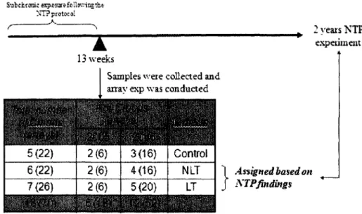
8. The experimental design of the Hamner lung tumor dataset 49
9. The box plot distribution of RMA normalized 70 array samples of Hamner 57
10. The box plot distribution of RMA normalised values for 178 array samples 61
11. Summarized view of the array outlier voting from different analysis groups 64
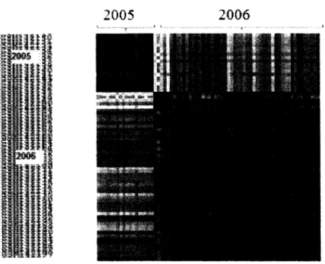
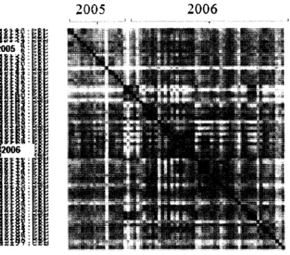
12. Correlation heat map of the Hamner lung tumor dataset with 70 arrays 66
13. Correlation heat map of the Hamner lung tumor dataset with 70 arrays after 67
14. Principal component analysis (PCA) of the Hamner lung tumor dataset 68
15. Q-Q plots for the Hamner dataset before correction of batch (top) and after 69
16. The above correlation heat maps for Hamner lung tumor dataset shows 70
17. The two-way ANOVA (LT_NLT and Batch label i.e. Year) results for Hamner.71
18. The correlation heat maps for Iconix liver cancer dataset 72
19. Principal component analysis (PCA) of Iconix liver cancer dataset 72
20. The two-way ANOVA (Class and Batch i.e. Year) results for Iconix 73
21. 512 differentially expressed genes (FC > 2 and P-value < 0.05) in NIEHS 76
22. 106 differentially expressed genes (FC>2 and P-value < 0.05) in MDACC 77 23. 197 differentially expressed genes (FC > 2 and P-value < 0.05) in MDACC 78
24. The schematic depiction of nested crossvalidation 85 25. The schematic diagram of the data analysis plan we studied 89
1. This table shows an example of gene expression data 14
2. dChip analysis results of the Hamner dataset which 57
3. dChip analysis results of the MDACC breast cancer 60
4. Consensus array outliers which are excluded from the further analysis 63
5. SVM and Naive Bayes (NB) classification performance 74
6. The differentially expressed genes passed the fold change 75
7. The five feature selection algorithms classification performance with six 81
8. Classification performance of three class (LT, NLT and Ctr) prediction 83
9. Classification performance of only two class (LT and NLT+Ctr) prediction 83
10. Classification performance of chemical compound based (multi class) 84
11. The classification performance and the best classifiers using nested cross 86
12. The classification performance and the best classifiers using nested 87
13. The table shows the top five models for the NT_NLT class (A) 90
14. The table shows the top five models for the Class (B) of the Iconix 91
15. The table shows the top five models for the Class (C) of the NIEHS 92
16. The table shows the top five models for the class pCR (D) of the MDACC 93
17. The table shows the top five models for the class erpos (E) of the MDACC 94
18. The table shows the top five models for the class O S M O (F) of the MM 95
19. The table shows the top five models for the class EFS_MO (G) of the MM 96
20. The table shows the top five models for the class CPS1 (H) of the MM 97
21. The table shows the top five models for the class CPR1 (I) of the MM 98
22. The table shows the top five models for the class OS_MO (J) of the NB 99
23. The table shows the top five models for the class EFS_MO (K) of the NB 100
24. The table shows the top five models for the class NEP_S (L) of the NB 101
25. The table shows the top five models for the class NEP_R (M) of the NB 102
CHAPTER I
INTRODUCTION AND BACKGROUND
The past two decades witnessed an explosive growth in biological information
generated by the scientific community. This was caused by major breakthrough advances
in the field of molecular biology, coupled with advances in genomic technologies. In
turn, the huge amount of genomic data not only leads to a demand on the computer
science community to help store, organize and index the data, but also leads to a demand
for specialized computational tools to view and analyze the data.1
"Biological science in the 21st century is being transformed from a purely lab-based science to an information science as well".
As a result of this transformation, a new field of science was born, in which
biology, computer science, and information technology merge to form a single discipline
called bioinformatics.
Motivation
Two decades ago, the main role of bioinformatics was to create and maintain
databases to store biological information, such as nucleotide and amino acid sequences.
With more and more data generated, nowadays, the most pressing task of bioinformatics
2
has moved to analysis and interpretation of various types of data, including nucleotide
and amino acid sequences, protein domains, protein structures and so on. To meet the
new requirements arising from the new tasks, researchers in the field of bioinformatics
are working on the development of new algorithms (mathematical formulas, statistical
methods, etc.) and software tools which are designed for assessing relationships among
large data sets, such as methods to locate a gene within a sequence, predict protein
structure and/or function and understand diseases at gene expression level.
In recent years, the rapid development of DNA microarray technology has made it
possible for scientists to measure the expression levels of thousands of genes in a single
experiment (Schena et al. 1995, Lockhart et al. 1996). Thus, DNA microarray technology
has found many applications in biomedical research. There are many active research
applications of this technology in clinical cancer research; it is being used to better
understand the biological mechanisms underlying oncogenesis (Butte 2002), in cancer
classification (predictors of good outcome versus poor outcome) (Golub et al. 1999;
Petricoin et al. 2002; van't Veer et al. 2002), clinical diagnosis (Yeang et al. 2001) and
in drug discovery studies. One of the main challenging tasks in this clinical cancer
research is the prediction of outcome, i.e., the potentiality of cancer regression and for
severe status (metastasis). The need for sensitive and reliable predictors of clinical
outcomes is crucial for early discovery of cancer patients. Identification of these clinical
outcomes has direct effect on the choice of optimal therapy for each individual (Perez et
Currently, there are two approaches to the computational analysis of gene
expression data for clinical classification purpose. The two approaches are discrimination
(supervised learning) and clustering (unsupervised learning). In unsupervised learning,
the classes are unknown and need to be discovered from the data (Brown et al. 2000).
This involves estimating the number of classes or clusters by using a clustering algorithm
such as hierarchical clustering (Eisen et al. 1998; Spellman et al. 1998) or self-organizing
maps (Tamayo et al. 1999) and assigning objects to these classes. In supervised learning
(also known as classification, supervised pattern recognition and class prediction), the
classes are predefined and the goal is to understand the basis for the classification from a
set of labeled data, also known as the learning set. This learned information is then used
to build a classifier or model, which will be used to predict the class or label of the future
unlabeled (blind) data, also known as external validation dataset (Dudoit et al. 2002).
Recently, significant research effort has been directed to the prediction of clinical
outcomes for several kinds of cancer on the basis of microarray data, which reported a
considerable success in this class prediction results (Bair et al. 2004; Beer et al. 2002;
Bhattacharjee et al. 2001; Khan et al. 2001; Ramaswamy et al. 2003; Rosenwald et al.
2002; Yeoh et al. 2002). But still there are two problems in this approach, the first is
when one analysis group's class model or predictor was tested on another group's same
type of cancer data, the success rate decreased significantly, and the second is
comparison of the marker gene lists used to predict a model by different groups revealed
4
The probable explanation for these problems may be due to several variables like
patient's age, race, sex, etc. and in the case of toxicological data like the amount of dose,
time, etc. Also, the platform of microarray technology used and the different methods of
data analysis play a significant role in these discrepancies (Ein-Dor et al. 2006; Michiels
et al. 2005), which we are studying extensively as one analysis group through
participating in the Microarray Quality Control Phase II (MAQC-II) project initiated by
the Federal Drug Administration (FDA).
Microarray Quality Control (MAQC) Project Overview of the Project
On March 16,2004, the US Food and Drug Administration (FDA) released a
report on "Innovation/Stagnation: Challenge and Opportunity on the Critical Path to
New Medical Products", addressing the recent slowdown in innovative medical products
submitted to the FDA for approval. The report described the urgent need to modernize
the medical product development process - the Critical Path from bench to bed side, and
they released the Critical Path Opportunities list that provided a concrete focus for public
and private efforts in new research development and tools. Among the 76 opportunities in
fields such as genomics, proteomics and bioinformatics, "Biomarker qualification" and
"Standards for microarray and proteomics-based identification of biomarkers" were
Microarray technology was identified by the FDA's Critical Path Initiative2 as a
key tool that holds "vast potential" for personalized medicine through the identification
of biomarkers. In response to the FDA's CPI, scientists at the FDA's National Center for
Toxicological Research (NCTR) formally launched the MicroArray Quality Control
(MAQC) project3 in order to address reliability concerns as well as other performance,
standards, quality and data analysis issues (Shi et al. 2006).
Microarray gene expression profiling is being used for a variety of applications,
two of which are (1) understanding general expression differences in various biological
populations, classes, states, or conditions, which typically leads to the identification of
lists of differentially expressed genes (DEGs) that distinguish populations and classes,
and (2) the development of predictive models or classifiers that accurately predict
outcomes of an individual based on a gene expression profile. These two types of
applications have important ramifications and distinctions. In the first, information about
a population or differences between populations is inferred. In the second, something
about an individual member of a population is inferred or predicted. Although signatures
can be used to classify individuals (e.g., assign or associate the individual with a subtype
of a particular disease), MAQC-II is primarily focused on prediction of health outcomes
based on microarray measurement of biological samples. These can putatively be used to
predict response to treatment regimens, patient prognosis, recurrence of disease, survival,
etc.
2 http://www.fda.gov/oc/initiatives/criticalpath/
6
MAQC -1 Findings: Microarrays Are Reproducible and Reliable
One important goal of the MAQC Phase I was to assess the best performance
achievable with microarray technology under consistent experimental conditions so that
future end users will have a benchmark to judge whether the quality of their microarray
data is comparable. A major challenge to the microarray user is the existence of
numerous options for analyzing the same data set, this is creating the reproducibility
problem (Eisenstein 2006). Even though, the reproducibility has seldom been, but in the
future should be used as a critical criterion to judge the performance of data analysis
procedures.
The MAQC-I analyses (Shi et al. 2006) demonstrated that the apparent lack of
reproducibility reported in previous studies (Marshall 2004; Tan et al. 2003) using
microarray assays was likely caused, at least in part, by the common practice of ranking
genes solely by a statistical significance measure, for example, P-values derived from
simple ^-tests, and selecting differentially expressed genes with a stringent significance
threshold, a result that is consistent with a previous report. The gene lists in the MAQC
study were much more concordant when fold change was used as the ranking criterion. In
addition, widely used statistical methods such as ranking based on false discovery rate
(FDR) values, t-test using SAM (significance analysis of microarray) did not appear to
improve inter-laboratory or inter-platform reproducibility compared to fold change
ranking. Importantly, non-reproducible gene lists could lead to inconsistent biological
interpretations, for example, in terms of enriched GO (Gene Ontology) terms and
to yield more reproducible signature gene lists. The effect of various data normalization
methods on the stability of lists of differentially expressed gene is greatly reduced when
fold change is used for gene selection.
M A Q C - 1 : Class Comparison -> What makesthe two populations different?
Normal Treated
5>
Differentially Expressed Genes
(DEGs)
Betterunderstandingof the biological mechanisms
M AQC - I I : Class Prediction -> Can the outcome of the new individuals be predicted?
li
Wm
Normal Cancer
Diagnosis, treatment outcome, prognosis, personalized medicine DEGs Predictive Models (Classifiers) Class prediction i I
i
f
UnknownFigure 1: Schematic representations of the two major types of applications of microarray technology are being addressed in Phase I (top image) and Phase II (bottom image) of the MAQC project, i.e., MAQC-I and MAQC-II, respectively.
8
Major findings of the first phase of the MAQC project were published in six
research papers on the September 8, 2006 issue of Nature Biotechnology (Canales et al.
2006; Guo et al. 2006; Patterson et al. 2006; Shi et al. 2006; Shippy et al. 2006; Tong et
al. 2006).
From MAQC-I to MAQC-II: To investigate the capabilities and limitations of
microarrays in clinical applications such as disease diagnosis, prognosis, treatment
outcome and personalized medicine, the MAQC Phase II (MAQC-II) has been launched
to address technical and scientific issues involved in the development and validation of
predictive models or classifiers (Figure 1). Multiple datasets were collected and
distributed for independent analyses to the participating organizations, in which the
University of Southern Mississippi (USM) group is also actively participating. The
results will normally be evaluated at three different levels: within a single dataset via
cross-validation, validation across one or more independent datasets from studies with the
same (or similar) study objectives, and validation with blinded "prospective" samples.
Objectives of MAQC-II
The overall goal of MAQC-II is to comprehensively evaluate different approaches
for the development and validation of predictive models or classifiers in clinical and
preclinical (toxicogenomics) applications by applying the same set of approaches to a
variety of datasets with diverse endpoints on which predictions are being developed. All
Clinical Applications:
1. Understand the behavior of various prediction rules and gene selection methods
that may be applied to microarray data sets to produce clinical outcome predictors: (a)
Examine the influence of the number of variables (probes or probe sets) on prediction
accuracy and robustness of the prediction result (in cross-validation and in independent
and "prospective" validation); (b) Examine the influence of prediction rules (algorithms)
on prediction accuracy and the robustness of prediction results (in cross-validation and in
independent validation); and (c) Examine robustness of prediction results in the face of
increasing experimental and artificial noise.
2. Identify and characterize the sources of variability in multi-gene prediction
results including (a) Inter- and intra-laboratory variation in prediction results (in replicate
experiments on the same platform); and (b) Cross-platform performance of prediction
results (in replicate experiments on different platforms). Only NIEHS (National Institute
of Environmental Health Sciences) is providing the datasets in two platforms (Affymetrix
and Agilent) generated using the same experimental setup.
Preclinical (toxicogenomics) Applications:
The primary goal is to assess the reliability of models for the prediction of toxicity
of new chemicals based on the microarray gene expression profiling. The entity to be
predicted is the toxicological endpoint (e.g., the presence or absence of liver toxicity) for
a chemical, and usually not for an individual animal. An important note is that in clinical
10
Design of MAQC-U
As part of the MAQC - II project, the FDA collected multiple datasets from
academic and industrial organizations. These datasets were distributed to the participating
organizations for independent analyses with available methodologies. We received these
datasets as part of the participating analysis groups after signing the Confidential
Information Disclosure and Transfer Agreements (CIDTA) from the USM contracts
office with the corresponding data providers.
The project is divided into four working groups for better coordination and
simplification for the participating organizations.
1. The Clinical Working Group (CWG) focuses on the datasets related to clinical
applications. The USM has been part of this CWG from the initial stages.
2. The Toxicogenomics Working Group (TGxWG) focuses on the datasets related to
toxicogenomics applications. The USM group has been part of this working group
from the beginning of this group.
3. The Titrations Working Group (TitrationWG) focuses on the datasets from
MAQC titration samples (including the MAQC-I Pilot data from 13 titration
mixtures). The USM group is not a participant in this working group.
4. The Regulatory Biostatistics Working Group (RBWG) provides recommendations
to the MAQC-II CWG and TGxWG on the process and criteria for evaluating the
performance of predictive models and classifiers. This working group evaluates
whether they are within the acceptable statistical framework or not. Before May
2007, the USM group along with other groups first proposed the Standard
Operating Procedures (SOPs) for each dataset separately as per the working
groups teleconference discussions. But after discussions and comments from the
RBWG on the loopholes in this approach (to have a separate plan for each dataset
would be biased) in the face-to-face meeting in SAS, Cary, NC in May 2007. The
statisticians' part of the RBWG unanimously recommended to the participating
analysis groups to prepare a single comprehensive Data Analysis Plans (DAPs)
for all the datasets from each group instead of separate plan for each dataset.
Datasetsfor Clinical and Toxicogenomics:
Datasets were identified for the purpose of evaluating
a) The performance of predictive models and classifiers (predictive signatures) and
b) The performance of different approaches and methodologies for algorithms
commonly used in the development of predictive models and classifiers.
Datasetsfor Clinical Working Group:
Three diseases, namely breast cancer (BR) from the M.D. Anderson Cancer
Center (MDACC), multiple myeloma (MM) from the University of Arkansas for Medical
Sciences (UAMS) and neuroblastoma (NB) from the University of Cologne, Germany,
were considered for more detailed examination for predictive modeling using microarray
data. I will explain in more detail about these datasets in the Materials and Methods
12
Datasetsfor Toxicogenomics Working Group:
The goal of the TGxWG is to develop and compare methods for deriving genomic
signatures from gene expression data that diagnose or predict toxicity of compounds in
animal models. It should be noted that the individual entities that will be predicted or
classified are individual chemicals, not individual animals.
Three datasets are selected to study under this working group. They are Lung
Tumor in rats from Hamner Institute, Hepatocarcinogenicity in rats from Iconix and
Overall necrosis score in mouse from NIEHS. These six datasets are explained in detail
in the Materials part of the chapter III of this dissertation.
Prediction and Classification Algorithms
Numerous algorithms have been reported in the literature for developing
prediction models and classifiers based on microarray gene expression data. The
Regulatory Biostatistics WG (RBWG) suggested more commonly (and possibly
appropriate) used methods to be evaluated with the MAQC-II datasets.
Supervised Learning and Classification Algorithms
Data mining is to extract implicit, previously unknown and potentially useful
information from data (Witten et al. 2000). It is a learning process, achieved by building
computer programs to seek regularities or patterns from data automatically. Machine
learning provides the technical basis of data mining. One major type of learning we
address in this dissertation is called classification learning, which is a generalization of
category given a set of positive class and negative class training instances of the category
(Mitchell et al. 1986). Thus, it infers a Boolean-valued function from the training
instances. As a more general format of the concept learning, classification learning can
deal with more than two class instances.
In practice, the learning process of classification is to find models that can
separate instances in the different classes using the information provided by training
instances. Thus, the models generated can be applied to classify a new unknown (blind)
instance to one of those classes. Stating it in simpler words, given some instances of the
positive class and some instances of the negative class, can we use them as a basis to
decide if a new unknown instance is positive or negative (Mitchell et al. 1986)?. This
kind of learning is a process from general to specific and is supervised because the class
labels of training instances are clearly known.
In contrast to supervised learning is unsupervised learning, where there are no
pre-defined classes or labels for training instances. The main goal of unsupervised
learning is to decide which instances should be grouped together, or in other words, to
form the classes. Sometimes, these two kinds of learning methods are used sequentially;
supervised learning makes use of class information derived from unsupervised learning.
This two-step strategy has achieved some success in the gene expression data analysis
field (Alizadeh et al. 2000; Golub et al. 1999), where the unsupervised clustering
methods were first used to discover classes (for example, subtypes of leukemia) so that
supervised learning algorithms could be employed to establish classification models and
14
Gene Expression Data Representation for Classification
In a typical classification task, data are represented as a table of samples (also
known as instances). Each sample is described by a fixed number of features (also known
as attributes, in our case, these were genes) and a label that indicates its class (Hall,
1998). For example, in studies of clinical outcome classification of cancer samples, gene
expression data of m genes for n cancer samples is often summarized by an n x (m+1)
table (X,Y) = (xy, yi), where xy denotes the expression level of gene/ in sample /, and yi
is the class or label (e.g., erpos in breast cancer) to which sample / belongs (i = 1,2,3,..., n
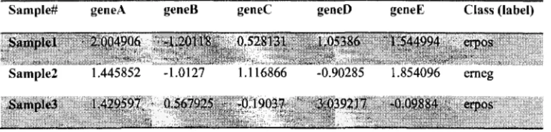
and/ = 1,2,..., m). The table (Table 1) below shows a sample dataset with three breast
cancer samples. Sample# Samplcl S;iin|)li2 Siiinpli'3 geneA 2.004906 1.445*52 1.429597 geneB -1.201 IS -I.DI2" 0.567925 geneC 0.528131 I.II6S66 -0.19037 geneD 1.05386 -0.90285 3.039217 geneE 1.544994 1.854096 -0.09884 Class (label) erpos crncg erpos
Table 1: This table shows an example of gene expression data. There are three samples, each of which is described by 5 genes. The class label in the last column indicates the clinical endpoint of the sample.
Results Evaluation or Error Estimation
Evaluation is the key to making real progress in supervised classification (Witten
et al. 2000). To evaluate the performance of classification algorithms, one way is to split
samples into two sets, training samples and test samples. Training samples are used to
build a learning model while test samples or external independent dataset (blind dataset)
dataset are supplied to the model, having their class labels "hidden", and then their
predicted class labels assigned by the model are compared with their corresponding
original class labels to calculate prediction accuracy. If two labels (actual and predicted)
of a test sample are same, then the prediction for this sample is counted as a success;
otherwise, it is an error (Witten et al. 2000). An often used performance evaluation term
is error rate, which is defined as the proportion of errors made over a whole set of test
samples. In some cases, we simply use the number of errors to indicate the performance.
Note that, although the error rate on test samples is often more meaningful to evaluate a
model, the error rate on the training samples is nevertheless useful to know as well since
the model is derived from them.
Predicted Neg Pos TN FN FP TP
Figure 2: Confusion matrix for two-class classification problem
Consider the confusion matrix illustrated in the above figure (Figure 2) of a
two-class ('Pos' and 'Neg') problem. The true positive (TP) and true negative (TN) are
correct classifications in samples of each class, respectively. A false positive (FP) is
when a 'Neg' class sample is incorrectly predicted as a 'Pos' class. A false negative (FN)
is when a 'Pos' class sample is incorrectly predicted as a 'Neg' class. Then each element of
a confusion matrix shows the number of test samples for which the actual class is the row
and the predicted class is the column. Thus, the error rate is just the number of false
positives and false negatives divided by the total number of test samples (i.e., error rate =
16
Error rate is a measurement of overall performance of a classification algorithm (also
known as a classifier); however, a lower error rate does not necessarily imply better
performance on a target task. For example, there are 10 samples in class 'Pos' and 90
samples in class 'Neg'. Suppose, if TP = 5 and TN = 85, then FP = 5, FN = 5 and the
error rate is 10%. However, only 50% of the samples are correctly classified in class
'Pos'. So, this is not a perfect evaluation metric in all cases. To more impartially evaluate
the classification results, some other evaluation metrics are constructed.
1. True positive rate (TP rate) = TP/(TP+FN), also known as recall or sensitivity,
measures the proportion of samples in class 'Pos' that are correctly classified as
class 'Pos'.
2. True negative rate (TN rate) = TN/(FP+TN), also known as specificity, measures
the proportion of samples in class 'Neg' that are correctly classified as class
'Neg'.
3. False positive rate (FP rate) = FP/(FP+TN) = 1 -specificity.
4. False negative rate (FN rate) = FN/(TP+FN) = 1-sensitivity.
5. Another evaluation metric in the classification studies is Matthews Correlation
Coefficient (MCC). We used this as our priority metric in determining the
candidate model for each end point as per the RBWG recommendation due to
more unbalanced classes for each endpoints in our study.
MCC takes into account true and false positives and negatives and is generally
different sizes (significantly unbalanced). It returns a value between -1 and +1. A
coefficient of+1 represents a perfect prediction, 0 an average random prediction and -1
the worst possible prediction (Baldi et al. 2000; Matthews 1975). Other measures, such as
the proportion of correct predictions, are not useful when the two classes are of very
different sizes. For example, assigning every object to the larger set achieves a high
proportion of correct predictions, but is not generally a useful classification.4
(TP*TN)- (FP*F.m MCC —
V'CTP + FP)(TP + FN)(TN + FP} (TN + FN}
In classification, it is a normal situation that along with a higher TP rate, there
comes a higher FP rate and same to the TN rate and FN rate. Thus, the receiver operating
characteristic (ROC) curve was invented to characterize the tradeoff between TP rate and
FP rate (Zweig et al. 1993). The ROC curve plots TP rate on the vertical axis against FP
rate on the horizontal axis. With an ROC curve of a classifier, the evaluation metric will
be the area under the ROC curve. The larger the area under the curve (AUC) (the more
closely the curve follows the left-hand border and the top border of the ROC space), the
more accurate the test. Thus, the ROC curve for a perfect classifier has an area of 1. The
expected curve for a classifier making random predictions will be a line on the 45 degree
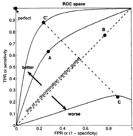
diagonal and its expected area is 0.5. Please refer to Figure 3 (figure slightly modified
from the courtesy image by Indon, 2007)5 for a sample ROC curve.
4 http://en.wikipedia.org/wiki/Matthews_Correlation Coefficient
18
ROC space
Figure 3: A sample ROC curve. The dotted line on the 45 degree diagonal is the expected
curve for a classifier making random predictions.
Error estimation methods
If the number of samples for training and testing is limited, a standard way of
predicting the error rate of a learning technique is to use stratified k-fold cross validation
(&-fold CV). In A>fold cross validation, first, a full data set is divided randomly into k
disjoint subsets of approximately equal size, in each of which the class is represented in
approximately the sample proportions as in the full dataset (Witten et al. 2000). Then the
above process of training and testing will be repeated k times on the k data subsets. In
remaining k-l subsets to build classification model, (3) the classification error of this
iteration is calculated by testing the classification model on the holdout set (Figure 4).
Finally, the k numbers of errors are added up to yield an overall error estimate.
Obviously, at the end of cross validation, every sample has been used exactly once for
testing.
A widely used selection for A:is 10. Why 10? "Extensive tests on numerous
different data sets, with different learning techniques, have shown that ten is about the
right number of folds to get the best estimate of error, and there is also some theoretical
evidence that backs this up"(Witten et al. 2000). Although 10-fold cross validation has
become the standard method in practical terms, a single 10-fold cross validation might
not be enough to get reliable error estimate (Witten et al. 2000). The reason is that, if the
seed of the random function that is used to divide data into subsets is changed, the cross
validation with the sample classifier and data set will often produce different results.
Thus, for a more accurate error estimate, it is suggested to repeat the 10-fold cross
validation process ten times and average the error rates. This is called 10-fold cross
validation with ten iterations and naturally, it is a computation-intensive undertaking.
First we used the 10-fold CV, but based on the recommendations from RBWG in 8th
face-to-face MAQC meeting, we choose to perform 5-fold CV with ten iterations because
the Hamner dataset is small and not strong data to use 10-fold with ten iterations. This
20
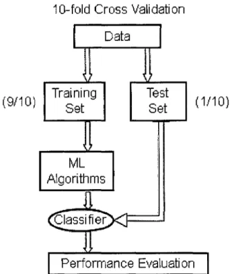
10-fold Cross Validation
(9/10) (1/10)
Performance Evaluation
Figure 4: A Graphical depiction of 10-fold cross validation
Instead of running cross validation ten times, another approach for a reliable results is
called leave-one-out cross validation (LOOCV). LOOCV is simply n-fold cross
validation, where n is the number of samples in the full data set. In LOOCV, each sample
in turn is left out and the classifier is trained on all the remaining n-\ samples.
Classification error for each iteration is judged on the class prediction for the holdout
sample, success or failure. Different from Mold (k < n) cross validation, LOOCV makes
use of the greatest possible amount of samples for training in each iteration and involves
Classification Algorithms
There are various ways to find models that separate two or more data classes, i.e.
to do classification. Models derived from the same sample data can be very different
from one classification algorithm to another. As a result, different models represent the
knowledge learned in different formats as well. For example, decision trees represent the
knowledge in a tree structure; instance-based algorithms, such as nearest neighbor, use
the instances themselves to represent what is learned; Naive Bayes method represents
knowledge in the form of probabilistic summaries. In this section, we will describe a
number of classification algorithms that have been used in this project, including NaiVe
Bayes, Support Vector Machines (SVM) and Voted Perceptron methods.
Support Vector Machines (SVM)
Support vector machines (SVM) is a kind of a blend of linear modeling and
instance-based learning (Witten et al. 2000), which uses linear models to implement
nonlinear class boundaries. It originates from research in statistical learning theory
(Vapnik, 1995). An SVM selects a small number of critical boundary samples from each
class of training data and builds a linear discriminant function (also called maximum
margin hyperplane) that separates them as widely as possible. The selected samples that
are closest to the maximum margin hyperplane are called support vectors. Then the
f(T~) discriminant function
for a test sample Tis a linear combination of the support vectors and it is constructed as:
22
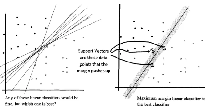
Any of these linear classifiers would be / Maximum margin linear classifier is fine, but which one is best? the best classifier
Figure 5: Graphical representation of Support Vector Machines concept
where the vectors Xz are the support vectors, } \ are the class labels (which are assumed to
have been mapped to 1 or -1) of Xu vector Trepresents a test sample. (Xc. T) is the dot
product of the test sample T with one of the support vectors Xt. «s and b are numeric
parameters (like weights) to be determined by the learning algorithm.
In the case that no linear separation is possible, the training data will be mapped into a higher-dimensional space H and an optimal hyperplane will be constructed there. The mapping is performed by a kernel function K(.,.) which defines an inner product in H
. Different mappings construct different SVMs (Figure 5). When there is a mapping, the
discriminant function is given like below which is a representation of a linear SVM.
An SVM is largely characterized by the choice of its kernel function. There are two types
of widely used kernel functions; polynomial kernel and Gaussian radial basis function
(RBF) kernel (Burges, 1998).
1. A polynomial kernel is if (Z1,X2) = {Kt.X2 + i)d, the value of power d is
called degree and generally is set as 1, 2 and 3. Particularly, the kernel
becomes a linear function if d = 1. It is suggested to choose the value of
degree starting with 1 and increment it until the estimated error ceases to
improve. However, it has been observed that the degree of a polynomial
kernel plays a minor role in the final results (Santos et al. 2002) and
sometimes, linear function performs better than quadratic and cubic
kernels due to over-fitting of the latter kernels.
2. An RBF kernel has the form KWi'*z) = e*P( is^t where a is the
width of the Gaussian. The selection of parameter a can be conducted via
cross validation or some other manners. When using SVM with RBF
kernel on gene expression data analysis, Brown group (Brown et al. 2000)
set a equal to the median of the Euclidean distances from each positive
samples (sample with class label as 1) to the nearest negative sample
(sample with class label as -1).
Besides polynomial kernel and Gaussian RBF kernel, other kernel functions include
sigmoid kernel (Scholkopf et al. 2002), locality-improved kernel (Zien et al. 2000) and so
24
/(T) = £ «,-y
iJfOf
ijr) + b
In order to determine parameters a and b in i , the
construction of the discriminant function finally turns out to be a constrained quadratic
problem on maximizing the Lagrangian dual objective function (Weston et al. 2001).
n i n
under constraints
n
«(yt =• 0, «j > 0, (i = 1,2, ...,n)
where « is the number of samples in training data. However, the quadratic programming (QP) problem in the above equation cannot be solved easily via standard techniques since it involves a matrix that has a number of elements equal to the square of the number of training samples.
Sequential Minimal Optimization (SMO)
To efficiently find the solution of the above QP program, Piatt developed the
sequential minimal optimization (SMO) algorithm (Piatt et al. 1998); one of the fastest
SVM training methods. Like other SVM training algorithms, SMO breaks the large QP
problem into a series of smaller possible QP problems. Unlike other algorithms, SMO
tackles these small QP problems analytically, which avoids using a time-consuming
numerical QP optimization as an inner loop. The amount of memory required by SMO is
linear with number of training samples (Piatt et al. 1998). Therefore it is good for large
I
datasets, as in our case, to take advantage of computationally inexpensive aspect. SMO
has been implemented into Weka, a data mining software package, which we used in this
study (Witten et al. 2000).
SVMs have shown to perform well in multiple areas of biological analysis, such
as detecting remote protein homologies, recognizing translation initiation sites (Liu et al.
2003; Zeng et al. 2002; Zien et al. 2000), and prediction of molecular bioactivity in drug
design (Weston et al. 2003). Recently, more and more bioinformaticians employ SVMs
in their research on evaluating and analyzing microarray expression data (Brown et al.
2000; Furey et al. 2000; Yeoh et al. 2002). SVMs have many mathematical features that
make them attractive for gene expression analysis, including their flexibility in choosing
a similarity function, sparseness of solution when dealing with large data sets, the ability
to handle large feature spaces, and the ability to identify outliers (Brown et al. 2000).
In many practical data mining applications, success is measured more subjectively
in terms of how acceptable the learned description rules, decision trees, or whatever are
to a human user (Witten et al. 2000). This measurement is especially important to
biomedical applications such as cancer studies where comprehensive and correct rules are
crucial to help biologists and doctors understand the diseases (Huiqing, 2004).
Naive Bayes
In machine learning, we are interested in determining the best hypothesis h(x)
from space H, based on the observed training data x. Best hypothesis is almost equal to
most probable hypothesis, given the data x with any initial knowledge about the prior
Bayes theorem provides a way to calculate,
(i) the probability of a hypothesis based on its prior probability Vx{h(x))
(ii) the probabilities of the observing various data given the hypothesis Pr(x|h)
(iii) the probabilities of the observed data Pr(x)
We can calculate the posterior probability h(x) given the observed data x,
Vx(h(x)\x)
using Bayes theorem.
. . .. , Fr(%lA6c))Pr(h(x))
PKAGO x) = r—rr
Pr(x)
Naive Bayes (NB) is a classification model obtained by applying a relatively simple
method to a training dataset (Mitchell et al. 1986). A NB classifier calculates the
probability that a given instance (example) belongs to a certain class. It makes the
simplifying assumption that the features constituting the instance are conditionally
independent, given the class.
Given an example X, described by its (xi> •••-• xn) feature vector we are
looking for a class Cthat maximizes the likelihood: P{X\C) = P(x±,...,xfl\£)
The (nai've) assumption of conditional independence among the features, given the class, allows us to express this conditional probability P(.X\ C) as a product of simpler
probabilities: P(X\C) = Hf=1 P O ^ I C ) . We used the Weka program to train the NB
classifier.
Voted Perceptron
The voted perceptron algorithm proposed by Freund et al. (1999) is based on the
Braverman and Rozonoer (1964), to run their algorithm efficiently in very high
dimensional spaces. This algorithm and its analysis involve little more than combining
these three known methods.
Their studies indicate that the use of kernel functions with the perceptron
algorithm yields a dramatic improvement in performance, both in test accuracy and in
computation time. In addition, they found that, when training time is limited, the
voted-perceptron algorithm performs better than the traditional voted-perceptron algorithm.
I discussed about the algorithms which I used for my final classification analysis in this
project. I have ignored the other algorithms in this discussion which we studied initially
for preliminary studies like KNN, Random Forest, J48 etc.
Feature Selection Algorithms
A well known problem in classification (in general machine learning) is to find
ways to reduce the dimensionality of the feature space to overcome the risk of
over-fitting especially when we are dealing with gene expression data. Data over-over-fitting
happens when the number of features (genes) is large ("curse of dimensionality") and the
number of training samples is comparatively small ("curse of data set sparsity"). In such
a situation, a decision function can perform very well on classifying training data, but
does poorly on test samples. Feature selection is concerned with the issue of
28
Categorization of feature selection algorithms
Feature selection techniques can be categorized according to a number of criteria
(Hall et al. 2003). One popular categorization is based on whether the target
classification algorithm will be used during the process of feature evaluation. A feature
selection method, that makes an independent assessment only based on general
characteristics of the data, is named "filter" (Witten et al. 2000); while, on the other hand,
if a method evaluates features based on accuracy estimates provided by certain
classification learning algorithm which will ultimately be employed for classification, it
will be named as "wrapper" (Kohavi et al. 1997, Witten et al. 2000). With wrapper
methods, the performance of a feature subset is measured in terms of the learning
algorithm's classification performance using just those features (see Figure 6 below).
The classification performance is estimated using the normal procedure of cross
validation, or the bootstrap estimator (Witten et al. 2000). Thus, the entire feature
selection process is rather computation intensive. For example, if each evaluation
involves a 10-fold cross validation, the classification procedure will be executed 10
times. For this reason, wrappers do not scale well to data sets containing many features
(Hall et al. 2003). Besides, wrappers have to be re-run when switching from one
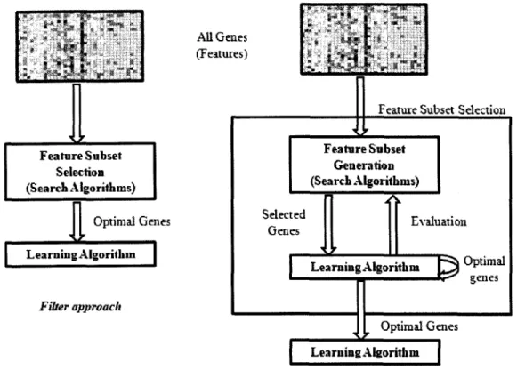
All Genes (Features) Feature Subset Selection (Search Algorithms) i £ Optimal Genes Learning Algorithm Fiber approach
1£
Feature Subset Selection
Feature Subset Generation (Search Algorithms) Selected Genes Evaluation • O I I LearningAlgorithm £ § °p t l m a l • •**' genes 1L Optimal Genes Learning Algorith m Wrapper approach
Figure 6: Graphical depiction of two feature selection (Filter and Wrapper) approaches.
In contrast to wrapper methods, filters operate independently of any learning
algorithm and the features selected can be applied to any learning algorithm at the
classification stage. Filters have been proven to be much faster than wrappers and hence,
can be applied to data sets with many features (Hall et al. 2003). Since the biological
data sets discussed in the later chapters of this dissertation often contain a huge number
of features (e.g., gene expression profiles), we not only concentrate wrapper but also
filter methods.
Another taxonomy of feature selection techniques is to separate algorithms
30
are some other dimensions to categorize feature selection methods. For example, some
algorithms can handle regression problem, that is, the class label is numeric rather than a
discrete valued variable; and some algorithms evaluate and rank features independently
from class, i.e., unsupervised feature selection (Witten et al. 2000). We will restrict our
study to the data sets with discrete class label since this is the case of the biological
problems analyzed in later chapters of this dissertation, though some algorithms
presented can be applied to numeric class label as well.
Feature selection algorithms
There are various ways and algorithms to conduct feature selection. We studied
five feature selection methods in this project; they are T-test, x statistical measure, gain
ratio, information gain and Relief-F.
T-test
Highly consistent with the well-known ANOVA principle, a basic concept for
identifying a relevant feature from an irrelevant one is the following: if the values of a
feature in samples of class 'A' are significantly different from the values of the same
feature in samples of class ' # ' , then the feature is likely to be more relevant than a feature
that has similar values in iA' and lB\ More specifically, in order for a feature/to be
relevant, its mean value in iA' should be significantly different from its mean value in
'fl'(Golubefa/. 1999).
The classical t-statistic is constructed to test the difference between means of two
t-statistic can be used to find features that have big difference in mean level between the
two classes. These features can be then considered to have ability to separate samples
between different classes (Nguyen et al. 2002). We tested this method in the initial stages
but did not perform well with over the other methods studied.
X2 - statistical measure
X2 measure evaluates features individually by measuring the x2 - statistic with
respect to the class. Different from the preceding methods, x2 measure can only handle
features with discrete values, x measure of a feature/with w discrete values is defined
as,
i—i L i C . f
i = l j - 1 *'
where k is the number of classes, Ati is the number of samples with /th value of/myth
E--
A--class. iJ is the expected frequency of lJ and
By = Ri * Cjfn
D
1 is the number of samples having /th value off, C, is the number of samples in they'th
class and n is the total number of samples.
We consider a feature/ to be more relevant than a feature/ (I £j) if y^(fj) > ^(fi).
Obviously, the worst x value is 0 if the feature has only one value. The
32
the degree of freedom known, the critical value for certain significant level can be found
from the appendix tables provided in most statistics books.
To apply x2 measure to numeric features, a discretization preprocessing has
to be taken. The most popular technique in this area is the state-of-art supervised
discretization algorithm developed by Fayyad and Irani (Fayyad et al. 1993) based on the
idea of entropy. At the same time, feature selection can be also conducted as a by-product
of discretization.
Information gain and Information gain ratio
Information gain is simply the expected reduction in entropy by partitioning
the samples according to this feature that it is the amount of information gained by
looking at the value of this feature. More precisely, the information gain Gain(f,S) of a
feature/, relatively to a set of samples S, defined as,
Gam(frS) = Ent(S) - Ent(f,Tf,S)
where Ent(S) can be calculated from
k
Ent(S) = y - pf * logzPt
and Ent(f, Tf, S) is the class entropy of the feature (for a numeric feature/, 2} is the best
partition t o / ' s value range under certain criteria, such as MDL principle in
discretization). Since Ent(S) is a constant once S is given, the information gain and
entropy measures are equivalent when evaluating the relevance of a feature. In contrast to
used in entropy measure, we consider a feature/ to more relevant than a feature// (I ^j) if
Gaintfj, S)>Gain(f,, S) (Xing et al. 2001, Quinlan 1986).
However, there is natural bias in the information gain measure - it favors
features with many values over those with few values. An extreme example is a feature
having different values in different samples. Although the feature perfectly separates the
current samples, it is a poor predictor on subsequent samples. One refinement measure
that has been used successfully is called information gain ratio. The gain ratio measure
penalizes features that with many values by incorporating amount of split information,
which is sensitive to how broadly and uniformly the feature splits the data (Mitchell et al.
1986).
E f t t ( 5 ) = 2j^ j - * logs
I£i1 |5| • "''* |5|
where Si through Sw are the w subsets of samples resulting from partitioning of S by
up-values discrete or w-value-interval numeric feature/ Then, the gain ratio measures is
defined in terms of the earlier information gain measure and this split information, as
follows:
GainRatio (f, S) =
Split Information (f, 5)
Note that split information is actually the entropy of S with respect to the
values of feature/and it discourages the selection of features with many values (Mitchell
et al. 1986). For example, if there is total number of n samples in S, the split information
of a feature/;, which has different values in different samples, is log2n. In contrast, a
34
information of 1. If these two features produce the equivalent information gain, then
clearly feature^ will have a higher gain ratio measure. Generally, a feature/ is
considered to be more significant than a feature/; (/ ±j) if GainRatio (f, S) >
GainRatio(fi, S). When using gain ratio measure (or information gain measure) to select
features, we sort the values of gain ratio (information gain) in the descending order and
consider those features with highest values.
ReliefF
The key idea of ReliefF is to estimate attributes according to how well their
values distinguish among the instances that are near to each other. For that purpose, given
an instance, ReliefF searches for its two nearest neighbors: one from the same class
(called nearest hit) and the other from a different class (called nearest miss). The original
algorithm of ReliefF (Kira et al. 1992) randomly selects n training instances, where n is
the user-defined parameter.
Chapter summary
In this chapter, I introduced the concept of classification in data mining as well as
the ways to evaluate the classification performance. I presented in detail some of
classification algorithms — putting the emphasis on several methods used in the final
analysis like SVMs, SMO and Naive Bayes. We also used KNN, Random forest, J48
algorithms to compare and contrast with the above algorithms in our preliminary studies
Also the basic concepts of feature selection algorithms and the differences
between filter and wrapper approaches were discussed. Also, the details about the feature
selection algorithms we studied like t-test, x2 statistic measure, Information gain,
36
CHAPTER II
MATERIALS AND METHODS
Methods
One of the important recent breakthroughs in experimental molecular biology is
microarray technology. This novel technology allows the monitoring of expression levels
in cells for thousands of genes simultaneously and has been increasingly used in cancer
research (Alizadeh et al. 2000; Alon et al. 1999; Golub et al. 1999) to understand more of
the molecular variations among tumors so that a more reliable classification becomes
possible.
There are two main types of microarray systems: the cDNA microarrays
developed in the Brown and Botstein Laboratory at Stanford (DeRisi et al. 1997) and the
high-density oligonucleotide chips from the Affymetrix company (Lockhart et al. 1996).
The cDNA microarrays (two-color) are also known as 'spotted' arrays, popularly called
as 'agilent' prepared from Agilent company (Miller et al. 2002), where the probes are
mechanically deposited onto modified glass microscope slides using a robotic array
machine. Oligonucleotide chips are synthesized in silico (e.g., via photolithographic
synthesis as in Affymetrix GeneChip arrays) are also popularly called as 'single channel'
arrays. For a more detailed introduction and comparison of the biology and technology of
the two systems, please refer to Harrington et al. (2000).
Gene expression data from DNA microarrays are characterized by many
samples), although both the number of experiments and genes per experiment are
growing rapidly (Nguyen et al. 2002). The number of genes on a single array is usually in
the thousands while the number of experiments is only a few tens or hundreds. There are
two different ways to view data: (1) data points as genes, and (2) data points as samples
(e.g., patients). In the way (1), the data are presented by expression levels across different
samples, thus there will be a large number of features and a small number of samples. In
the way (2), the data is represented by expression levels of different genes, thus the case
will be a large number of samples with a few attributes. In this dissertation, all the
discussions and studies on gene expression profiles are based on the format of data
presentation that is data points as genes or features.
Microarray experiments raise many statistical questions in many diversified
research fields, such as image analysis, experimental design, cluster and discriminant
analysis, and multiple hypothesis testing. The main objectives of most microarray studies
can be broadly classified into one of the following categories: class comparison, class
discovery, or class prediction (Miller et al. 2002).
Class comparison is to establish whether expression profiles differ between
classes. If they do, which genes are differentially expressed between the classes, i.e. gene
identification. For example, which genes are useful to distinguish tumor sample from
non-tumor ones. This is the typical microarray analysis we will perform every day.
Class discovery is to establish subclusters or structure among specimens or among
38
Class prediction is to predict a phenotype using information from a gene
expression profile (Miller et al. 2002). This includes assignment of malignancies into
known classes (tumor or non-tumor) or tumor samples into already discovered subtypes,
prediction of patients outcome such as which patients are likely to experience severe drug
toxicity versus who will have none, or which breast cancer patients will relapse within
five years of treatment versus who will remain disease free.
In this dissertation, we will focus on the class comparison and class prediction.
For these two tasks, supervised analysis methods that use known class information are
most effective (Miller et al. 2002). In practice, feature selection techniques are used to
identify discriminatory genes while classification algorithms are employed to build
models on training samples and predict the phenotype of blind test cases.
Preprocessing of Expression Data
Despite optimal techniques to ensure RNA quality, some amount of
non-biology-related variation remains; thus, preprocessing of the microarray data is essential before
analysis can be initiated. Several critical preprocessing techniques have been developed
to enhance the validity of microarray analyses. Based on the characteristics of the
experimental data, the normal preprocessing steps include identification of outlier arrays,
scale transformation, data normalization, missing value management, batch effect
correction, replicate handling and so on (Herrero et al. 2003).
Identification of Outlier Samples
Array outliers are due to excessive chip-to-chip variation and may be the result of