Peer effects in English Primary schools: An IV estimation on the effect of a more able peer group on age 11 examination results

THE CENTRE FOR MARKET AND PUBLIC ORGANISATION

Centre for Market and Public Organisation Bristol Institute of Public Affairs

University of Bristol 2 Priory Road Bristol BS8 1TX http://www.bristol.ac.uk/cmpo/ Tel: (0117) 33 10752 Fax: (0117) 33 10705 E-mail: cmpo-office@bristol.ac.uk

The Centre for Market and Public Organisation (CMPO) is a leading research centre, combining expertise in economics, geography and law. Our objective is to study the intersection between the public and private sectors of the economy, and in particular to understand the right way to organise and deliver public services. The Centre aims to develop research, contribute to the public debate and inform policy-making.

CMPO, now an ESRC Research Centre was established in 1998 with two large grants from The Leverhulme Trust. In 2004 we were awarded ESRC Research Centre status. CMPO is now wholly funded by the ESRC.

ISSN 1473-625X

Peer effects in English Primary schools:

An IV estimation of the effect of a more able peer group

on age 11 examination results

Steven Proud

October 2010

CMPO Working Paper Series No. 10/248

Peer effects in English Primary schools:

An IV estimation on the effect of a more able peer group

on age 11 examination results

Steven Proud1

1

CMPO and Department of Economics, University of Bristol

November 2010

Abstract

The magnitude and characteristics of the effect of a child’s peers on their outcomes has long

interested researchers and policy makers. In this paper, I take advantage of the correlation between the average outcomes a child’s peer group attains with the distribution of ages within the cohort to construct an instrument for the ability of the peer group in order to estimate the peers effects on children’s outcomes at age 11. IV results suggest there is a significant positive effect of a more able peer group. Furthermore, the results suggest that there is more benefit for children who are close to the ability of the peer group than those whose ability is not close.

Keywordspeer groups, primary education JEL ClassificationI21, I38, J24

Electronic version www.bristol.ac.uk/cmpo/publications/papers/2010/wp248.pdf Acknowledgements

I would like to thank the Department for Education for access to the National Pupil Database. Thanks also go to Professor Simon Burgess and Dr Deborah Wilson, and to participants at seminars in the Centre for Market and Public Organisation for helpful comments. Also, to the Economic and Social Research Council who provided funding for this research as part of a PhD in Economics.

Address for correspondence Steven Proud

Centre for Market and Public Organisation University of Bristol

2 Priory Road Bristol BS8 1TX

Steven.Proud@bristol.ac.uk www.bristol.ac.uk/cmpo/

1

1 Introduction

The Coleman report (Coleman et al 1966) brought to attention the possibility that the make-up of a child’s peer group has a significant effect on their academic outcomes. Furthermore, Coleman et al (1966) suggest that outcomes are determined, in decreasing magnitude, by pupils’ family background, attributes of the peer group and finally attributes of the school and teachers.

Since the Coleman report, many papers have tried to measure the effect of a various aspects of the peer group on individuals’ academic outcomes, with the most common being the mean prior ability of the peer group. However, since Manski (1993) recognised the inherent endogeneity of peer ability the process of which identifying the effect of a more able peer group has been recognised as difficult. Three main strategies have been employed to solve the endogeneity problem: controlling for large amounts of heterogeneity (e.g. Zimmer and Toma (2000)); assuming credibly random assignment of students (e.g. Zimmerman (2003)); finding a credibly exogenous instrument to take advantage of two stage least squares. (e.g. Lefgren (2004)). However, the majority of prior research concentrates on the effect of the peer group being linear-in-means, there has been a handful of recent studies that has suggested that a linear specification is more appropriate. Gibbons and Telhaj (2008) suggest such non-linear specifications, with the higher and middle ability students gaining more proportionately from an increase in the ability of the peer group compared with low ability students. Similar evidence of non-linearity is suggested by Hoxby and Weingarth (2005).

There is strong evidence that pupils’ outcomes in compulsory national assessments are strongly influenced by their month of birth, (Sharp (1995), Crawford et al (2007), Strom (2004)), with the oldest pupils within the year group performing better than their younger peers. In England, these differences are usually attributed to the older pupils gaining more maturity as they sit the examinations when they are older than the younger pupils. This correlation between individual outcomes and month of birth suggests also that a peer group that consists largely of older pupils will, in general, have higher previous outcomes.

This paper uses an identification strategy which takes advantage of the correlation between the month of birth and outcomes in externally assessed examinations, with pupils born in September having an advantage over those born in August to carry out an instrumental variables analysis of the effect of a more able peer group on the outcomes of children at age 11. I take advantage of a within school estimation, conditioning on prior achievement.

2

Furthermore, I suggest that the observed effects are credibly the effect of a more able peer group, rather than being confused with the effect of an individual having an older peer group. I contend that whilst it may be advantageous for children to be born in September, the proportion of pupils born in each third of the year is essentially random, and this is backed up by the Hansen J test of overidentifying restrictions, which suggests that the instrument is credibly exogenous in all specifications. In order to examine the possibility of non-linearities of the effect of a more able peer group, I consider differential effects, depending on the difference between the child’s ability and the average ability of the peer group. Further, in order to examine the direct effect of a more able peer group within classrooms, I use a characteristic of English schools. That is, I classify schools with 30 or fewer pupils within the cohort as schools with credibly only one class per cohort. As such, all of the pupils within the school-year can be defined as the peer group who are taught in direct contact with each individual pupil. Additionally, this paper examines differential effects of a more able peer group on pupils who are close in terms of ability to the ability of their peer group and on pupils whose ability is a long way from the ability of their peers. Testing of the validity of the instrument suggest that it is exogenous in all specifications, and I find significant, non-trivial, positive effects of having a more able peer group on results at key stage 2 in English and mathematics, with a larger effect being observed in mathematics than in English. Furthermore, the results suggest that in both English and mathematics the strongest effects of a more able peer group are observed for children who have prior outcomes that are close to the average outcome of their peer group, with a reduced effect observed for pupils who are a long way from the ability of their peer group. However, the effects look roughly symmetrical around the peer group, with only the pupils who have outcomes which are a long way above the ability of the peer group in English within small schools showing insignificant effects.

I begin by discussing some of the recent literature related to the estimation of peer effects using instrumental variables, and also the correlation of age within year and ability or outcomes. Further to this, I also briefly discuss prior literature of other applications where age has been considered as an instrument for ability within education. I then look at specific data issues faced from the PLASC dataset utilised in this research, and the specifics of the data required for the statistical analysis. Section 4 will examine the methodology used, whilst section 5 will discuss the results gained from the statistical analysis, and I will finish with conclusions based on the results and further discussion.

3

2 Literature

In this section, I discuss in a little more detail previous studies estimating the effect of a more able peer group, and the motivation for the use of age as an instrument.

Examining studies which take advantage of instrumental variables methods to estimate the effect of a more able peer group, Lefgren (2004) uses an instrument constructed from the degree to which schools group pupils according to ability, and finds evidence of very small positive effects from a more able peer group. Robertson and Symons (2003) use region of birth dummies as instruments for the effect of different socioeconomic status students on pupils’ outcomes, and suggest that there are advantages to be had from having peers of a higher socioeconomic status. Angrist and Lang (2004) use an instrument based on the predicted number of METCO students in a class under a US relocation programme, and find little effect of an influx of lower ability pupils into the school.

The research that comes closest to the research I consider here is by Maurin et al (2005), which take advantage of the correlation between outcomes and age within year to estimate the effect of the peer group on outcomes. They use the percentage of pupils born in each month to try to identify the effect of the peer group. Their analysis suggests that the peer effect is non-linear, but they cannot disentangle whether the effect they are observing is from being with peers of higher ability, or whether the observed effect is from being grouped with older children. Similar research is conducted by Sandgren and Strom (2005), who examine the effect of the average age of the peer group on children’s outcomes, and find a significant effect in mathematics and reading, with the effect more robust for male students than for female students. However, they do not try to examine the effect of a more able peer group.

In this paper, I use the proportion of pupils within the peer group who are in the oldest third of the age distribution and the proportion of pupils who are in the youngest third of the age distribution as instruments for the ability of the peer group. However, for this to be a valid strategy, two conditions need to be met. That is, there needs to be an appreciable correlation between the proportion of pupils in the cohort within each third of the age distribution and the outcomes of the peer group, and that the instruments are not correlated with the error terms.

In the past, the correlation between student outcomes and the age of the student has been taken advantage as an instrument by several studies. For example, Atkinson et al (2006) use

4

age within year as an instrument for whether a pupil attends a grammar school or not. They state that “Within year age has a direct effect on attainment at 16: in both selective and non-selective LEAs, older pupils achieve higher GCSE scores” (Atkinson et al (2006,25)). Similarly, Angrist and Krueger (1991) use the age of a child within a school year based on the quarter of the year in which they are born as an instrument for education level. They find no significant difference from their OLS results. However, Angrist and Krueger’s approach is criticised by Bound et al (1995) who demonstrate that Angrist and Krueger’s results are strongly affected by including additional instruments in the analysis, and their results are subsequently biased due to their instruments being weak. However, Angrist and Krueger’s choice of instrument tries to capture the length of time students spend in education, due to the fact in some US states; all children start school at the same time, but are allowed to leave school directly after their 16th birthday. This system is not reproduced in the UK, and as discussed above, there is an appreciable difference in outcomes associated with the birth-date of the child.

To further reinforce the strong correlation between the age make-up of the peer group and the ability of the peer group, Crawford et al (2007) analyse the impact of when a child is born on outcomes in English schools. They compare outcomes for children within schools who are born in September with those born in August, and control for other factors that are likely to affect children’s outcomes. They find that August born boys and girls are at a significant disadvantage to their September born peers, but that this disadvantage decreases over time. They quantify that at age 5, August born boys are 0.817 standard deviations (SDs) behind September born boys, whilst August born girls are 0.768 SDs behind September born girls. However, by age 16, this has decreased to August born boys being 0.131 SDs behind their September born counterparts, whilst for girls; the penalty of being born in August is 0.116 SDs. Furthermore they examine pupils with special educational needs, including both children with statements of special educational needs and children with non-statemented special educational needs. They find that at age 11, August born girls are 25% more likely to have statements of special educational needs, whilst the boys are 14% more likely to have statements. However, this difference falls back at age 16. However, they argue that the identification of these special educational needs, particularly for those non-statemented children may simply be due to them progressing at a slower rate than their older peers. They argue that the major reason for the August-born penalty is that August born children are essentially a year younger than their September born counterparts when they sit the tests. These issues are now widely recognised amongst UK policy makers (see BBC (2008)). Following this review, the secretary of state responsible for education within the Department for Children, School and Families (DCSF) launched a review of primary education, and the minister

5

suggested that summer born children should be allowed to defer their entry into school by up to a year.

Similarly, looking at English data, Sharp (1995) examines the effect of season of birth on outcomes at both key stage 1 and GCSE examinations, and finds that the eldest children within the schools perform best in these assessments. Likewise, Sharp et al (1994) consider the effect of season of birth on academic outcomes at age 7. They find that the oldest pupils perform best, but their analysis is clouded by some of the younger pupils only having eight terms of education, compared with their peers who have received nine terms of education.

Further weight to the argument that August-born children are likely to perform worse in academic testing is added by Strom (2004), which examines the effect of birth-date on children’s outcomes in formal testing at age 15-16. He finds a significant disadvantage for the youngest children in reading compared with their older classmates.

Considering the exogeneity of the age of the peer group; For the choice of instrument to be valid, it requires the month of birth to be credibly exogenous. Whilst there is a danger that some parents may try and influence the date of birth of their child, (See, for example BBC (2009)), it must be remembered that whilst they may have a preference, this is countered by difficulties in conception and by unintended pregnancies. Ford et al (2000) suggest that 28.7% of pregnancies in the Avon area are unintended, whilst Scheike and Jensen (1997) suggest that 59% of planned pregnancies take longer than 1 month to achieve conception. Further to these difficulties in achieving pregnancies, the time of birth is also difficult for parents to control, with 8.6% of UK births registered as premature, and only 33.7% of births occurring at the expected 40 weeks1. These factors suggest that the distribution of births will be credibly random. Furthermore, Dickert-Conlin and Elder (2010) suggest that, in the US at least, there is little evidence of parents manipulating the date of birth of their child, and find no discontinuities of maternal characteristics based on school cutoff dates.

3 Data

This paper uses data from the Pupil Level Annual School Census (PLASC) and the National Pupil Database (NPD). The NPD is an administrative database, and was established in 2002, and

1 _{Premature birth indicates born before 37 weeks gestation. Source of statistics HES online, available at}

http://www.hesonline.nhs.uk/Ease/servlet/AttachmentRetriever?site_id=1937&file_name=d:\efmfiles\193 7\Accessing\DataTables\Maternity\Tables%2021%20to%2030\Tb27\Mat_Tb27_0708.xls&short_name= Mat_Tb27_0708.xls&u_id=8441 accessed on 15/09/09

6

allows us to observe pupils’ outcomes in national testing at ages 7, 11, 14 and 16. Further, the database contains data on the pupils’ date of birth, sex, ethnicity, whether they have English as a first language, their special educational needs (SEN) status, their free school meals status (FSM), and also contains some school level data, including the number of pupils within the school and number of full time teachers. In England, children are usually taught in primary schools, from age 4 until age 11 and then in secondary schools from age 11 onwards. Primary schools are also separated into infant schools from age 4 to 7 and junior schools from age 7 to 11. Since primary schools are generally much smaller, the children experience more direct contact with their peer group than in secondary schools, and so this makes primary schools the natural environment in which to conduct this study. Within primary schools, pupils are assessed at the end of two national curriculum stages, key stage 1 (KS1) and key stage 2 (KS2). At KS1, pupils have been explicitly examined in reading, writing and mathematics, whilst at key stage 2, they were examined in English mathematics and science.

This paper takes advantage of data for pupils in this dataset were examined in key stage 2 examinations between 2002 and 2006, and were examined in key stage 1 examinations between 1998 and 2002. These key stage 1 test scores are necessary to model the ability of the peer group.

At key stage 1, pupils are examined in reading, writing and numeracy. In order to create measures of English and mathematics, I consider the reading and writing as a composite English score, simply consisting of the average national curriculum level that the child achieved, and for mathematics, I simply take the numeracy score. These levels are subsequently normalized to mean zero and standard deviation of 1. These levels gained at key stage 1 and key stage 2 are associated with descriptions of pupils achievement levels within the national curriculum2. However, it needs to be remembered that these key stage 1 scores are essentially discrete data, so an individual key stage 1 score can cover a relatively large range of abilities.

The scores I use here at key stage 2 are a much finer score, based on the raw score in the examination. However, these scores are not directly linked to a national curriculum level fixed across years. That is, the raw mark required in an examination to achieve a certain level one

22 _{See, for an example of current national curriculum levels}

http://curriculum.qcda.gov.uk/key-stages-3-

and-4/subjects/mathematics/keystage3/Copy_of_index.aspx?return=/key-stages-3-and-4/subjects/mathematics/keystage3/index.aspx%3Freturn%3D/key-stages-3-and-4/subjects/index.aspx , accessed 2nd October 2009

7

year is not necessarily the same score that is required in a subsequent year3. As such, this raw score is normalised by year to have the same mean and standard deviation as the national curriculum level score. As the national curriculum score is comparable across years, this can then normalised to have a mean of 0 and standard deviation of 1. This normalised raw score allows for a better comparison of outcomes of pupils than the very discrete and clustered measure of the national curriculum level achieved, where a pupil who achieves a good score within a level is classified the same as a pupil who achieves a borderline score in that level.

Whilst this strategy would also be desirable with the explanatory variable of key stage 1 achievement, the data is not currently available to consider a more continuous score. However, within the broad national curriculum level that the pupils achieve, there is also a smaller break-down into levels a, b and c, showing the pupils progression towards the next level.

The identification strategy I pursue requires that the peer test-score measure is correlated with the average age of the cohort, but that the average age of the cohort is uncorrelated with the error term. As such, it would be beneficial if the pupils are essentially randomly assigned to schools by age, and that parents do not try to maximise their children’s outcomes by trying to ensure their children are the oldest within the academic year. For this identification strategy to be credible, therefore we want there to be randomness on when children are born within the year, and so would expect an even spread of the month in which children are born (Although we would expect February to have significantly fewer births than October, since there are 28 (or 29) days in February, compared with 31 in October.

Figure 1 shows the distribution of the age of pupils at the start of the year when they take their key stage 2 examinations, based on month of birth. Key stage 2 examinations are sat in year 6, which is the academic year when pupils turn 11. There are small numbers of pupils who are in the wrong academic year based on their year of birth, but the vast majority of pupils are in a class with pupils born in the same academic year. In order to control for possible mis-codings of birth year, pupils who, in the raw data, are recorded as starting year 6 younger than age 9 or older than age 12 are dropped from the data. Whilst it might be hoped that the months of birth provide a perfect uniform distribution, this is not entirely the case, for several reasons. It is immediately apparent that there are fewer births in February than in any

3

For example, a mark of 43 at key stage 2 English in 2003 would have achieved a level 3, whilst the same mark in 2004 would have gained a level 4.

8

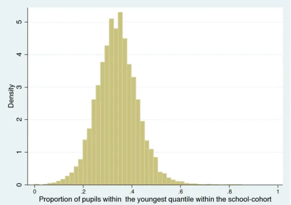
other month, but this is simply due to the fact that February is the shortest month4. There are also more than expected births in September5. However, when considering pupils born in the three quantiles of age based on months of birth shown in Figure 2 we can see that the distribution of births across the year is approximately equal. Figure 3 shows the distribution of the proportion of the within school cohort who are defined to lie in the youngest third of the age distribution, whilst Figure 4 shows the distribution of the proportion of the within school cohort who are defined to lie in the oldest third of the age distribution. These follow similar approximately normal distributions, as would be expected.

In order to reduce selectivity into schools, I only consider schools that have a comprehensive admissions policy, and the sample only consists of schools which are foundation, community, voluntary aided and voluntary controlled schools. Further to this, in some local authorities, there are a number of schools which select pupils according to ability. However, whilst the remaining schools in these local authorities have a comprehensive admissions policy, they have had the cream skimmed off the top, and as such would not have a representative distribution of pupils. In order to prevent this, I consider local authorities with 10 percent or more of their pupils selected by ability to be selective authorities, and remove these from the sample. Finally, in order to reduce the possibility of my results being affected by junior schools teaching some pupils in mixed year classrooms, or by excessively small schools, I omit any school that has fewer than 10 pupils registered.

4 Methodology

I begin with a general educational production function, considering pupils’ attainment at key stage 2 to be a function of school inputs, consisting of school policy effects, teacher effects, and peer ability effects, family inputs and demographics affecting the ability of the child to learn effectively.

There are a large number of factors that are likely to be constant within a school, such as the neighbourhoods in which the children grow up, and there will be high correlation between pupils in the level of parental income within neighbourhoods and schools. Furthermore, all of the pupils within the schools are taught in the same atmosphere, with the same facilities available to them, with the same teaching culture that is engendered by the head teacher. As

4 _{We would expect the proportion of births in February to be 0.077 (2sf). The observed proportion we see}

here is 0.077 (2sf)

5

The proportion within our sample who are born in September is 0.087, compared with a theoretically random proportion of 0.082.

9

such, it is necessary to try to control for these factors, which may also be correlated with the ability of the peer group, but which are not directly observable within my data. In order to control for these correlated between school heterogeneities, I use similar techniques to Hanushek et al (2003) and McEwan (2003), and include school fixed effects.

As such, I model attainment A at time t for individual i in school k to be a function of prior attainment, individual demographics, X, school effects, S, within school cohort effects, C, (such as peer ability spillover) and error terms, u.

Here, I include lagged ability as t-4 since I am examining the effects of a more able peer group on outcomes at age 11. Pupils’ prior achievement can thus be modelled from their key stage 1 examinations, sat at the age of 7, that is, 4 years previously.

) , , , , ( _{4, , ,} ,ik t ik tik kt k tik t f A X C S u A = ₋ (14)

This research considers the effect of being in a school with a more able peer group. There is still the worry that, despite having included school fixed effects, there are elements within the error term that are correlated with both the outcome at age 11 and the prior ability of the peer group. In order to mitigate this correlation, and the resultant bias inherent I use a similar strategy to Sandgren and Strom (2005) and Maurin et al (2005). I use two stage least squares to estimate the effect of a more able peer group. I use the proportion of pupils within the school-year who lie in the oldest third and the proportion of pupils within the school-year who are in the youngest third of the age distribution as instruments for the average within year school average score at 7.

The first stage of the two stage least squares is estimated thus:

it t k ikt ikt i j k t k i j a ageave X KS s t u classave _{≠, ,−4} = + _{, ≠}

β

β

where classave is the average key stage 1 score of the pupils in English (or mathematics) gained in school k, by all of the pupils j at time t-4. ageave is a vector containing the proportion of pupils within the school cohort that are in the top third of the age distribution and the proportion of pupils who lie within the bottom third of the age distribution. s is a school level fixed effect and t is a dummy for the year that the students sit the key stage 2 examination and u is a random error term. There is little variation within the school cohort of the classave variable, as the only variation comes from the omission of individual pupils.

10

Since we expect there to be correlations between the explanatory variables at a school level, due to factors explained above, it is necessary to adjust the standard errors to mitigate the problems when the independent and identically distributed assumptions are dropped. In order to control for these effects, I cluster the standard errors at school level.

As discussed in section 2, we would expect there to be a correlation between the ages of pupils within the cohort with their individual outcomes. That is, we would expect the oldest pupils to gain the highest grades at key stage 1. Therefore, we would also expect a cohort with a high proportion of ‘old’ pupils to have a better average outcome than a cohort with a high proportion of ‘young’ pupils. As such, we would expect the proposed instruments to be strongly correlated with the ability of the peer group. Since the standard errors are clustered at the school level, this implies that the observations are no longer independent and identically distributed, and as such, I need to appeal to the methods proposed by Kleibergen and Paap (2006) in order to test for underidentification of the endogenous variables. (see Baum et al (2007)). As such, I use the Lagrange multiplier (LM) test proposed by Kleibergen and Paap (2006) to test for underidentification. Since the sample is close to a population, there is little worry that if we reject the null of underidentification that there will be a problem with weak instruments. However, I do calculate the Kleibergen Paap F-statistics and compare them with the critical values calculated by Stock and Yogo (2005), but do not report them here.

I estimate the second stage of the two stage least squares thus

it t k it it t i j k ikt classave X KS s t KS2 =

α

γ

γ

γ

ε

Where KS2 is the individual pupil’s (i) score at key stage 2 in English or mathematics. X is a vector of individual level characteristics, including pupil age, gender at time t and exam scores at time t-4 (pupils take their key stage 2 examinations 4 years after their key stage 1 examinations)in English and mathematics at key stage 1.

In order to test the exogeneity assumptions, I appeal to statistical testing. Standard testing methods would appeal to the Sargan statistic. However, Baum et al (2007) suggest that since I consider the possibility that there is correlation within clusters at school level, the Hansen J statistic is the correct statistic to consider when examining the test of overidentifying restrictions. That is, whether the instruments are truly exogenous.

11 4.1 Small schools versus large schools

In order to accurately assess the effect of a more able peer group, it may not be sufficient to simply examine entire schools. This is due to the fact that in large schools, there may be no interaction between pupils in different classrooms within the school. In order to try to observe pupils who are taught together, I use a characteristic of English infant schools, which is discussed in detail in Proud (2008). From 2002 onwards, it has been a legal requirement that classrooms within infant schools in England have a maximum of 30 pupils within the class. Proud (2008) suggests that there is strong evidence that schools that have 30 or fewer pupils within the school cohort consist of just 1 class per academic year. That is, since the PLASC data does not include classroom level data, I need to try to infer where pupils are directly taught with their entire school cohort. As such, in order to infer these classrooms, I consider schools that only contain 30 or fewer pupils in every cohort, which indicates that each year, the school only fills up one classroom, and then closes admissions.

4.2 Differential effects on different ability of pupils.

Previous studies have looked at differential effects of a more able peer group on outcomes for high ability and low ability children, for example Zimmer and Toma (2000). In order to examine this possibility, I consider the effect on individuals whose key stage 1 results are either close to the average outcome for their peer group, or for individuals who are far away from the mean ability of their peer group. To do this, I construct a new variable that measures the distance away from the peer group ability that an individual is, and construct quartiles of this distance on all of the individuals in the data

5 Summary Statistics

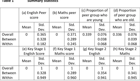
Table 1 shows summary statistics for the key stage 2 outcome variables, the prior attainment at key stage 1, the peer ability measure (as measured by the average of the peers’ scores at age 7), and the proportion of pupils within the peer group who lie in the oldest and youngest thirds of the age distribution within the school. The summary statistics are broken down into overall, between and within standard deviations.

As discussed within the data section, the key stage 1 and key stage 2 scores are normalised with mean 0 and standard deviation of 1. For this analysis, it is important that there is a significant variation within school of the peer ability measure. If not, then the peer ability will

12

simply be absorbed by the inclusion of a school-level fixed effect. The distribution of the peer ability measure is shown in sections (a) and (b) of Table 1. Since the key stage 1 scores are normalised, then the mean of the peer scores is also zero. The standard deviation of the peer ability measure for English overall is 0.365 and the standard deviation of the peer ability measure for mathematics overall is 0.371. What is key is whether there is any variation within schools of this peer ability measure. For English, the standard deviation within school is 0.182, which makes up 24.8% of the total variance of the peer ability measure, whilst for mathematics, the standard deviation is 0.245, which makes up 43.5% of the total variance of the peer ability measure. As such, whilst the majority of the variation in the peer ability score is between school (56.6%-75.5%), there is still a significant within school variation in the ability of the peer group.

Similarly, in order for my instrument to be useful, there needs to be within school variation of the proportion of pupils who are in the oldest third of the age distribution and the proportion of pupils who are in the youngest third of the age distribution. The distribution of the proportion of pupils within the age thirds is shown in sections (c) and (d) of Table 1. Whilst the overall standard deviation is low, there is a range of proportions of pupils between 0 and 1 within the oldest third, and a range of pupils between 0 and 0.9 in the youngest third. In terms of the proportion of the variance in these proportions that is observed within schools, for the proportion of pupils who are in the youngest third, 80% of the variance is within the schools, and similarly 80% of the overall variance is within schools for the oldest third of the cohort. Furthermore, sections (e)-(h) of Table 1 suggest that 88% of the variance in the key stages 1 and 2 scores are within schools, which is as would be expected.

6 Results.

In this section I will initially discuss the OLS and IV results for English and mathematics, initially examining the simple all school specification. I will then look at the effects for schools with a large distribution of examination scores, and examine differential effects of being in a class with a more able peer group if you are close to the ability average ability of the peer group and if you are far away from the ability of the peer group.

I am interested in the estimates of the coefficients from equation (16):

it t k it it t i j k ikt classave X KS s t KS2 =

α

γ

γ

γ

ε

13

I am particularly interested in the coefficient γ0 . In order to correct for possible endogeneity

of the peer ability measure (classave), it is also necessary to consider a two stage least squares estimation using equation (15)

it t k ikt ikt i j k t k i j a ageave X KS s t u classave _≠, ,₋4 = + , _≠

β

β

Results of the first stage regressions will only be reported for the most general specification.

6.1 OLS Results

Table 2 gives OLS estimates of the effect of a more able peer group on outcomes in English and mathematics at key stage 2. In examining these results, I will begin by describing the estimates of the effects from the other explanatory variables, that is the variables which we do not suspect are endogenous, and will then move on to the estimates of the effect of a more able peer group.

As would be expected, we see a significant positive effect of own prior achievement on outcomes at key stage 2. For English, specification (ii) implies that a one standard deviation increase in prior achievement is associated with a 0.602 standard deviation increase in their key stage 2 scores, whilst a 1 standard deviation increase in maths scores at key stage 1 is associated with a 0.182 standard deviation increase in their English key stage 2 score. Furthermore, we can observe a strong negative effect of poor socioeconomic status, modelled by whether the child has free school meals. Also, in English, ceteris paribus, being male lowers the outcome at key stage 2 by 0.15 standard deviations. The only coefficient that isn’t in the direction that might be expected is on the age of the child within the year. The direction of this coefficient can be explained by the fact that I have controlled for prior attainment. This is explained in Crawford et al (2007) that the gap between the oldest and the youngest decreases as the children get older6. Considering the effects of variables that we consider to be exogenous in mathematics, a similar set of effects are observed. The magnitude of the negative effect of free school meals is the same in mathematics, although, there is a stronger negative effect of an older pupil in mathematics. The largest difference is in whether the pupil is male or not. Having controlled for prior ability and age, boys perform 0.188 standard

6 _{As a robustness check it is possible to consider the specification both with prior achievement controlled}

for, and without prior achievement controlled for. The introduction of the prior achievement switches the direction of the coefficient on age from positive to negative.

14

deviations better than girls in mathematics. However, this is as would be expected. Boys initially perform better in mathematics than girls, but this advantage is eroded over time. Finally, the prior achievement in English has marginally more effect on pupils’ achievement at key stage 2 in mathematics than the prior attainment in mathematics had on scores at key stage 2 for English.

In terms of the effect of a more able peer group, Table 3 suggests that for both English and mathematics, a more able peer group is related to a reduction of the outcome at key stage 2, with a magnitude of a 1 standard deviation increase in the peer group outcome leading to approximately a 0.1 standard deviation decrease in the key stage 2 outcome score. However, it must be remembered that these estimates are likely to be correlated with the error term, and as such are likely to be a mis-estimate.

6.2 Two stage least squares Results.

Table 3 gives results from the first stage of the two stage least squares estimation of the effect of a more able peer group on outcomes at age 11 for all pupils within all schools. In examining these results, I will begin by discussing whether the instruments I have used are plausibly valid based on econometric testing, and will conclude by discussing the effects of a more able peer group. As would be expected, the estimates of the effects of the variables that we do not suspect are endogenous are largely the same as those in the OLS estimation case.

The results presented here suggest a statistically significant negative correlation between the proportion of pupils who are young within the cohort and the peer ability measure, and a statistically significant positive correlation between the proportion of pupils who are old within the cohort and the average ability of the peer group. As such we would expect to reject the null of underidentification. Table 4 gives the results from the second stage of the two stage least squares for all pupils in all schools. For both English and mathematics, we can observe a significant and non-trivial positive effect of a more able peer group on outcomes at age 11 Reported in Table 4 are tests on the validity of the instruments under these specifications. As expected, based on the results from the first stage regressions, the P values on the Kleibergen-Paap test of underidentification are 0.0000 for both specifications (1) and (2) for both English and mathematics, and so we reject the null of no correlation between the instrument and the peer ability measure. The presence of a large sample and the size of the

15

Kleibergen Paap LM test suggest that weak instruments should not be a problem. However, to check this, I compare the Kleibergen Paap Wald F statistic with the 10% maximal IV size statistic from Stock and Yogo (2005).7 Table 4 also reports the Hansen-J test of the overidentifying restrictions. In both specifications, for both English and mathematics, we fail to reject the null that the instruments are not correlated with the error term. Since we reject the null of underidentification, and fail to reject the null of endogeneity of the instruments, our instruments appear to be valid.

Examining the results from specification 1 and 2 for English in Table 4 imply that a 1 standard increase in the ability of the peer group is related to a 0.0423 standard deviation increase in the outcomes that a child achieves at key stage 2. Similarly, an increase in the peer group outcome in mathematics by one standard deviation is related to an increase in a pupil’s key stage 2 in mathematics score of between 0.0516 and 0.0597 standard deviations.

6.3 Results in small schools

As discussed in the methodology section, whilst we would like to observe directly the effect of a more able peer group within the classroom, this if often not possible, as for a large proportion of schools, we cannot directly observe which pupils are taught in a classroom with which. In order to estimate the classroom level effect, I consider here schools which have fewer than 30 pupils in all observed cohorts as a proxy for schools which teach all of their pupils in one class (which I describe here as a small primary school) Table 5 shows the results for all pupils who are educated within small primary schools. By placing the restriction on the size of the school, I have removed 8,863 schools from the sample (74.4% of the sample), but we are still left with a large sample of children within the population (326,654 children in the sample).

Again, it is important to check the validity of the instruments. As with the all school sample, we strongly reject the null of no correlation of the instruments with the endogenous variables, and we also strongly fail to reject the null that the instruments are not correlated with the error term, so the tests support the argument that the instruments are valid.

7 _{The Kleibergen-Paap F-statistics are calculated and compared with the Stock-Yogo critical values, and}

we reject the null of weak instruments at all reasonable levels of significance. These statistics are greater than the 10% maximal IV size in all samples.

16

The estimates of the effect of the exogenous variables are of the same magnitude as those observed in the full sample case, as is the estimate of the effect of a more able peer group. However, in contrast with the full sample case, there is only a significant positive effect of a more able peer group in specification (ii) for mathematics, and there is no significant effect within small schools of a more able peer group.

6.4 Results for pupils based on difference from the average of the peer ability.

It would be advantageous to see if all pupils are affected in the same way by an increase in the ability of the peer group. That is, whether children who are a long way above the ability of their peer group would benefit as much from an increase in the ability of their peer group as children who are close to the ability of the peer group. For analysis here, I consider 4 quartiles of the distance of an individual pupils’ key stage 1 score and the average key stage 1 score of their peers. Specification (a) is the lowest quartile below the ability of the peer group, (b) is the second quartile, (c) the third, and (d) is the highest quartile above the average outcome of the peer group.

Table 6 shows the results from all schools for English of the effect of a more able peer group on sub-groups of the population. Again, for all specifications, the tests for validity of the instruments reject the null of underidentification, and fail to reject the null in the test of overidentifying restrictions, indicating that the instruments are valid. Examining the coefficients on the effect of a more able peer group suggests that pupils who are closer to the ability of the peer group are affected more by an increase in the prior outcomes of their peer group than those who are a long way away. For specification (a), a 1 standard deviation increase in the average outcome of the peer group is associated with between a 0.115 and 0.119 standard deviation increase in a pupil’s outcomes at key stage 2. Similarly, specification (b) suggests a 1 standard deviation increase in the peer ability is related to a between 0.154 and 0.165 standard deviation increase in the individual’s outcomes. Specification (c) suggests a between 0.194 and 0.196 standard deviation increase, whilst specification (d) suggests between a 0.069 and 0.074 standard deviation increase from a 1 standard deviation increase in the peer ability measure.

Table 7 shows the effect of a more able peer group, broken down by distance from the peer ability outcome. Again, tests on the instruments indicate that there is no problem with underidentification, nor with endogeneity of the instruments. The effects are of similar magnitudes to those seen in all schools, but the major difference is that in small schools, it

17

appears that the most able students (i.e. the students whose ability is highest above the average ability of their peer group) do not gain any statistically significant advantage from being educated with a more able peer group.

Table 8 shows the estimates for a more able peer group in mathematics, again broken down by the distance of the individual pupil from the average ability of their peer group. The Kleibergen Paap and Hansen-J tests again do not find any problems with the instruments, indicating that the instruments are not invalid. The effect of other, exogenous, variables is of the same magnitude as that seen in the whole school regressions, other than for specification (b). Here, it appears that prior ability has no effect. Furthermore, these results suggest that an increase in peer ability will have a considerably larger effect on your own outcomes than for any other group. Comparing with sub-sample (a), for whom a 1 standard deviation increase in the peer ability measure is related to a between 0.167 and 0.181 standard deviation increase in key stage 2 score, for sub-sample (b) a 1 standard deviation increase in the peer ability measure is associated with between a 0.453 and a 0.459 standard deviation increase in the outcomes at key stage 2 in mathematics. As with English, sub-samples (c) and (d) see a reduction in the effect of a more able peer group on individuals’ outcomes at key stage 2.

Table 9 shows the results within small schools, and shows a similar structure of effects, with the largest effects of a more able peer group once again seen for children who are close to the ability of the peer group, albeit below (i.e., sub-sample (b)). As with English, the significance of the effect of a more able peer group is reduced for sub-sample (d): that is, pupils whose outcomes at key stage 1 mathematics are a long way above those of the peer group.

6.5 Summary

In all of the specifications, I have rejected the null of underidentification and failing to reject the null of the excluded instruments being exogenous. These tests send a strong signal that the instruments are valid, and that there will be less bias from the IV estimates than from the OLS estimates. The IV estimates of the effect of a more able peer group suggest that an increase in the ability of the peer group by one standard deviation is related to an increase in the outcomes at key stage 2 by between 0.04 and 0.4 standard deviations. There is little difference between the estimates obtained within small schools and schools overall. However, it is clear that the strongest effect is observed for pupils who are close to the ability of their peer group.

18

7 Conclusions.

In this paper, I have examined the effects of a more able peer group on individuals’ outcomes at age 11, with a sample of both full schools, but I also try to estimate the effect of a more able peer group, dependent on how far away from the ability of the peer group the child’s own ability is. I have taken advantage of an instrument proposed by Angrist and Krueger (1991) as the age make-up of the peer group as an instrument for their ability. Whilst Sandgren and Strom (2005) suggest that there may be more mechanisms than just ability operate when considering the effect of an older peer group on outcomes, my results show no evidence of any endogeneity of the instruments used. The results presented here suggest significant and non-trivial positive effects of a more able peer group on individual children’s outcomes at age 11.

Estimates from the instrumental variables specifications suggest that a 1 standard deviation increase in the prior achievement of the peer group is related with a between 0.04 and 0.4 standard deviation increase in the outcome the individual achieves at key stage 2. Furthermore, the results presented suggest that pupils who are close to the ability of their peer group are benefitted more from an increase in the ability of the peer group than those whose ability is further away from the ability of the peer groups. Also, the results here imply that pupils who are a long way below the ability of their peer group are improved more by an increase in the peer group ability than those who are a long way above the ability of the peer group. This result is similar for the highest and lowest ability pupils to that presented by Zimmer and Toma (2000), who suggest that there is a greater effect of a higher ability peer group on lower ability pupils than for higher ability pupils, but this is in contradiction to the effect on high achievers observed by Gibbons and Telhaj (2008) suggest that there is a positive effect of a more able peer group on the highest and middle ability, but those at the bottom of the ability distribution are largely unaffected by an increase in the ability of the peer group.

The previous literature examining the effect of a more able peer group on children’s academic outcomes has been unable to reach a consensus on the effect of an increase in the mean ability of the peer group, with results ranging from no, or a very small significant effect (e.g. Angrist and Lang (2004) (No effect of a less able peer group introduced), Lefgren(2004b) (a 1 standard deviation increase in the peer ability measure linked with a 0.024 standard deviation increase in individuals outcomes), to a much larger effect of a magnitude of a 1 standard deviation increase in peer ability related to a 0.3 standard deviation increase in individual’s

19

achievement (e.g. Kang 2007)). Further studies have suggested effects within this range (e.g. Hoxby (2000) suggests a 1 standard deviation increase in peer ability is related to a between 0.05 and 0.14 standard deviation increase in the outcome of individual students, whilst Gibbons and Telhaj (2008) suggest that for middle achieving students, a 1 standard deviation increase in the proportion of pupils who are high achievers is related to a 0.15 standard deviation increase in their outcomes. Similarly Hanushek et al (2003) suggests a 0.1 standard deviation increase in the peer ability measure is associated with a 0.02 standard deviation increase in individuals’ outcomes.

The results obtained here for English are of a similar magnitude to those estimated by Hanushek et al (2003) and Hoxby (2000). The results obtained for mathematics largely tell a similar story, other than for the pupils who are close, but below, the ability of their peer group. This group experiences a larger effect, but it is still of similar magnitude to that estimated in Kang (2007).

20

References

Angrist, J. D., and Krueger, A. B. (1991): Does Compulsory School Attendance Affect Schooling and Earnings, Quarterly Journal of Economics, 106(4), 979-1014.

Angrist, J. D., and Lang, K. (2004): Does School Integration Generate Peer Effects? Evidence from Boston's Metco Program, American Economic Review, 94(5), 1613-34.

Atkinson, A., Gregg, P., and Mcconnell, B. (2006) The Result of 11 Plus Selection: An Investigation into Opportunities and Outcomes for Pupils in Selective LEAs, CMPO Working Paper 06/150, Centre for Market and Public Organisation, University of Bristol Baum, C. F., Schaffer, M. E., and Stillman, S. (2007): ivreg2: Stata module for extended instrumental variables/2SLS, GMM and AC/HAC, LIML, and k-class regression, Boston College Department of Economics, Statistical Software Components S425401. Downloadable from http://ideas.repec.org/c/boc/bocode/s425401.html.

BBC (2008): Summer-born to start school later, http://news.bbc.co.uk/1/hi/education/7178969.stm accessed on 06/07/2009

BBC (2009): Is this the worst day of the year to be born?, http://news.bbc.co.uk/1/hi/magazine/8227268.stm accessed on 11/09/09

Bound, J., Jaeger, D. A., and Baker, R. M. (1995): Problems with Instrumental Variables Estimation When the Correlation between the Instruments and the Endogenous Explanatory Variable Is Weak, Journal of the American Statistical Association, 90(430), 443-450.

Coleman, J. S., Campbell, E. Q., J., H. C., Mcpartland, J., M., M. A., D, W. F., and L, Y. R. (1966) Equality of Educational Opportunity, OE-38001 and supp., US Department of Health, Education & Welfare, Washington, DC.

Crawford, C., Dearden, L., and Meghir, C. (2007) When you are born matters: the impact of date of birth on child cognitive outcomes in England, Discussion Paper 93, LSE/Centre for the Economics of Education

Dickert Conlin, S and Elder, Todd (2010): Suburban legend: School cutoff dates and the timing of births, Economics of Education Review 29(5), 826-841.

Ford, W. C. L., North, K., Taylor, H., Farrow, A., Hull, M. G. R., Golding, J., and Team, A. S. (2000): Increasing paternal age is associated with delayed conception in a large population of fertile couples: evidence for declining fecundity in older men, Human Reproduction, 15(8), 1703-1708.

Gibbons, S., and Telhaj, S. (2008) Peers and achievement in England’s secondary schools, SERC Discussion Paper 1, Spatial Economics Research Centre

Hanushek, E. A., Kain, J. F., Markman, J. M., and Rivkin, S. G. (2003): Does peer ability affect student achievement?, Journal of Applied Econometrics, 18(5), 527-544.

Hoxby, C. (2000) Peer Effects in the Classroom: Learning from Gender and Race Variation, NBER Working Paper 7867, National Bureau of Economic Research

21

Kang, C. H. (2007): Classroom peer effects and academic achievement: Quasi-randomization evidence from South Korea, Journal of Urban Economics, 61(3), 458-495.

Kleibergen, F., and Paap, R. (2006): Generalized reduced rank tests using the singular value decomposition, Journal of Econometrics, 133(1), 97-126.

Lefgren, L. (2004): Educational Peer Effects and the Chicago Public Schools, Journal of Urban Economics, 56(2), 169-91.

Manski, C. F. (1993): Identification of Endogenous Social Effects: The Reflection Problem,

Review of Economic Studies, 60(3), 531-42.

Maurin, E., Mcnally, S., and Ouazad, A. (2005) Peer Effects in English Primary Schools, Economics of Education and Education Policy in Europe Conference, Uppsala University and the Institute for Labor Market Policy Evaluation (IFAU)

Mcewan, P. J. (2003): Peer effects on student achievement: evidence from Chile, Economics of Education Review, 22(2), 131-141.

Proud, S. (2008) Girl Power? An analysis of peer effects using exogenous changes in the gender make-up of the peer group., CMPO Working Paper 08/186, Centre for Market and Public Organisation, University of Bristol

Robertson, D., and Symons, J. (2003): Do peer groups matter? Peer group versus schooling effects on academic attainment, Economica, 70(277), 31-53.

Sandgren, S., and Strom, B. (2005) Peer effects in primary school: Evidence from age variation, Annual Conference EALE, Prague

Scheike, T. H., and Jensen, T. K. (1997): A discrete survival model with random effects: An application to time to pregnancy, Biometrics, 53(1), 318-329.

Sharp, C. (1995): Whats Age Got to Do with It - a Study of Patterns of School Entry and the Impact of Season of Birth on School Attainment, Educational Research, 37(3), 251-265. Sharp, C., Hutchison, D., and Whetton, C. (1994): How Do Season of Birth and Length of

Schooling Affect Childrens Attainment at Key Stage-1, Educational Research, 36(2), 107-121.

Stock, J., and Yogo, M. (2005): Testing for Weak Instruments in Linear IV Regression. In D. W. K. Andrews, and J. H. Stock Identification and Inference for Econometric Models: Essays in Honor of Thomas Rothenberg (pp. 80–108). Cambridge: Cambridge University Press. Strom, B. (2004) Student achievement and birthday effects, CESifo-Harvard University/PEPG

Conference on "Schooling and Human Capital in the Global Economy: Revisiting the Equity-Efficiency Quandary", CESifo Conference Center, Munich

Zimmer, R. W., and Toma, E. F. (2000): Peer Effects in Private and Public Schools across Countries, Journal of Policy Analysis and Management, 19(1), 75-92.

Zimmerman, D. J. (2003): Peer Effects in Academic Outcomes: Evidence from a Natural Experiment, Review of Economics and Statistics, 85(1), 9-23.

22

Figure 1 Distribution of month of birth of pupils

23

Figure 3 Distribution of the proportion of pupils within school who are in the youngest third of the age distribution

Notes: Unit of observation is the proportion of students within the total school cohort who is born in the youngest of three quantiles. One observation per school

Figure 4 Distribution of the proportion of pupils within a school cohort lie within the oldest third of the age distribution.

Notes: Unit of observation is the proportion of students within the total school cohort who is born in the oldest of three quantiles. One observation per school

24

Table 1 Summary Statistics

(a) English Peer score

(b) Maths peer score

(c) Proportion of peer group who

are young

(d) Proportion of peer group who are old. Mean Std. Dev. Mean Std. Dev. Mean Std. Dev. Mean Std. Dev. Overall 0 0.365 0 0.371 0.339 0.076 0.336 0.076 Between 0.328 0.289 0.038 0.039 Within 0.182 0.245 0.068 0.068

(e) Key Stage 1 English Score (f) Key Stage 1 Maths score (g) Key Stage 2 English (h) Key Stage 2 Maths Mean Std. Dev. Mean Std. Dev. Mean Std. Dev. Mean Std. Dev. Overall 0 1 0 1 0 1 0 1 Between 0.328 0.289 0.354 0.341 Within 0.949 0.960 0.941 0.945

Notes. The unit of comparison is at pupil level. Between indicates variation between schools, within indicates variation within schools as a whole, both within and across cohorts.

Table 2 OLS estimation for all pupils in all schools

English Mathematics

(i) (ii) (i) (ii)

Average English KS1 score of peer group

-0.269*** -0.280*** -0.364*** -0.329*** (0.006) (0.006) (0.005) (0.004) Child takes free school

meals -0.122*** -0.114*** -0.151*** -0.094*** (0.001) (0.001) (0.001) (0.001) Age of child -0.056*** -0.103*** -0.137*** -0.180*** (0.002) (0.002) (0.002) (0.002) Male pupil -0.108*** -0.153*** 0.098*** 0.188*** (0.001) (0.001) (0.001) (0.001) Key stage 1 English

score 0.728*** 0.602*** 0.277*** (0.001) (0.001) (0.001) Key stage 1 mathematics score 0.182*** 0.720*** 0.534*** (0.001) (0.001) (0.001) Observations 2446348 2446348 2446348 2446348 Number of schoolid2 11919 11919 11919 11919 R-squared 0.56 0.58 0.53 0.57

Notes. Dependent variable is the individual pupils’ key stage 2 score in English or mathematics. Method of estimation is ordinary least squares. Standard errors, clustered at school level are in parentheses. * denotes significance at the 10% significance level; ** denotes significance at the 5% significance level; *** denotes significance at the 1% significance level. School level fixed effects are included. Dummies are included for the individual’s ethnic group and the year in which the pupil sits the examination.

25

Table 3 First stage regressions for all pupils in all schools.

English Mathematics

(i) (ii) (i) (ii)

Proportion of pupils in the youngest quantile

-0.200*** -0.200*** -0.237*** -0.237*** (0.013) (0.013) (0.015) (0.015) Proportion of pupils in

the oldest quantile.

0.158*** 0.158*** 0.188*** 0.187*** (0.013) (0.013) (0.015) (0.015) Child takes free school

meals 0.006*** 0.006*** 0.008*** 0.006*** (0.000) (0.000) (0.000) (0.000) Age of child -0.009*** -0.010*** -0.016*** -0.015*** (0.000) (0.000) (0.001) (0.001) Male pupil 0.005*** 0.004*** -0.001*** -0.005*** (0.000) (0.000) (0.000) (0.000) Key stage 1 English

score 0.009*** 0.007*** -0.011*** (0.000) (0.000) (0.000) Key stage 1 mathematics score 0.004*** 0.021*** 0.029*** (0.000) (0.000) (0.000) Observations 2446348 2446348 2446348 2446348 Number of schoolid2 11919 11919 11919 11919 R-squared 0.13 0.13 0.36 0.36

Notes. Dependent variable is the average of the peer group’s results at key stage 1 in English or mathematics. The proportion of pupils in the youngest third and the proportion of pupils in the oldest third are introduced as excluded instruments for the average key stage 1 score of the peer group. Method of estimation is ordinary least squares. Standard errors, clustered at school level are in parentheses. * denotes significance at the 10% significance level; ** denotes significance at the 5% significance level; *** denotes significance at the 1% significance level. School level fixed effects are included. Dummies are included for the individual’s ethnic group and the year in which the pupil sits the examination.

26

Table 4 IV estimation in all schools.

English Mathematics

(i) (ii) (i) (ii)

Average key stage 1 score of peer group

0.116** 0.116** 0.139*** 0.162***

(0.047) (0.047) (0.037) (0.036)

Child takes free school meals -0.125*** -0.117*** -0.155*** -0.097*** (0.001) (0.001) (0.001) (0.001) Age of child -0.052*** -0.098*** -0.127*** -0.171*** (0.002) (0.002) (0.002) (0.002) Male pupil -0.110*** -0.154*** 0.099*** 0.190*** (0.001) (0.001) (0.001) (0.001)

Key stage 1 English score 0.724*** 0.599*** 0.283***

(0.001) (0.001) (0.001)

Key stage 1 mathematics score

0.181*** 0.710*** 0.520***

(0.001) (0.001) (0.001)

Underidentification test 719.065 719.430 751.626 752.298

P-value 0.0000 0.0000 0.0000 0.0000

Weak instrument test

statistic 393.716 393.934 413.768 414.147

Stock Yogo Critical value 19.93 19.93 19.93 19.93

Hansen J statistic of overidentifying restrictions 0.616 0.536 0.263 0.072 P value 0.4324 0.4642 0.6082 0.7887 Observations 2446348 2446348 2446348 2446348 Number of schoolid2 11919 11919 11919 11919

Notes. Dependent variable is the individual pupils’ key stage 2 score in English or mathematics. Method of estimation is two stage least squares. Excluded instruments for the average key stage 1 score of the peer group are the proportion of pupils who are in the youngest third and the proportion of pupils within the oldest third of the age distribution within the peer group. Standard errors, clustered at school level are in parentheses. * denotes significance at the 10% significance level; ** denotes significance at the 5% significance level; *** denotes significance at the 1% significance level. School level fixed effects are included. Dummies are included for the individual’s ethnic group and the year in which the pupil sits the examination. The underidentification test is the Kleibergen Paap LM Test. The weak instrument test statistic is the Kleibergen Paap Wald F statistic. The Stock Yogo critical value is the 10% maximal IV size.

27

Table 5 IV estimation within small schools.

English Mathematics

(i) (ii) (i) (ii)

Average key stage 1 score of peer group

0.103 0.098 0.092 0.121**

(0.074) (0.074) (0.061) (0.059)

Child takes free school meals -0.121*** -0.113*** -0.147*** -0.093*** (0.004) (0.004) (0.004) (0.004) Age of child -0.053*** -0.100*** -0.125*** -0.167*** (0.004) (0.004) (0.005) (0.005) Male pupil -0.109*** -0.153*** 0.097*** 0.187*** (0.002) (0.002) (0.003) (0.003)

Key stage 1 English score 0.705*** 0.583*** 0.270***

(0.002) (0.002) (0.002)

Key stage 1 mathematics score 0.178*** 0.683*** 0.501*** (0.002) (0.003) (0.003) Underidentification test statistic 218.222 218.224 259.362 259.412 P-value 0.0000 0.0000 0.0000 0.0000

Weak instrument test

statistic 121.640 121.639 148.077 148.089

Stock Yogo Critical value 19.93 19.93 19.93 19.93

Hansen J statistic of overidentifying restrictions 0.049 0.074 0.042 0.095 P value 0.8254 0.7852 0.8369 0.7584 Observations 326455 326455 326455 326455 Number of schoolid2 3056 3056 3056 3056

Notes. Dependent variable is the individual pupils’ key stage 2 score in English or mathematics. Method of estimation is two stage least squares. Excluded instruments for the average key stage 1 score of the peer group are the proportion of pupils who are in the youngest third and the proportion of pupils within the oldest third of the age distribution within the peer group. Standard errors, clustered at school level are in parentheses. * denotes significance at the 10% significance level; ** denotes significance at the 5% significance level; *** denotes significance at the 1% significance level. School level fixed effects are included. Dummies are included for the individual’s ethnic group and the year in which the pupil sits the examination. A small school is defined as a school that has 30 or fewer pupils in every observed cohort. The underidentification test is the Kleibergen Paap LM Test. The weak instrument test statistic is the Kleibergen Paap Wald F statistic. The Stock Yogo critical value is the 10% maximal IV size.