Modeling recommendations for pattern-based mashup plans

University of Stuttgart Universitätsstraße 38

D–70569 Stuttgart

Master Thesis

Modeling Recommendations for

Pattern-based Mashup Plans

Somesh Das

Course of Study: Computer Science

Examiner: Prof. Dr.-Ing. habil. Bernhard Mitschang Supervisor: Dipl.-Inf. Pascal Hirmer

Commenced: October 17, 2017 Completed: April 17, 2018

Data mashups are modeled as pipelines. The pipelines are basically a chain of data processing steps in order to integrate data from different data sources into a single one. These processing steps include data operations, such as join, filter, extraction, integration or alteration. To create and execute data mashups, modelers need to have technical knowledge in order to understand these data operations. In order to solve this issue, an extended data mashup approach was created–FlexMash developed at the University of Stuttgart–which allows users to define data mashups without technical knowledge about any execution details. Consquently, modelers with no or limited technical knowledge can design their own domain-specific mashup based on their use case scenarios.

However, designing data mashups graphically is still difficult for non-IT users. When users design a model graphically, it is hard to understand which patterns or nodes should be modeled and connected in the data flow graph. In order to cope with this issue, this master thesis aims to provide users modeling recommendations during modeling time. At each modeling step, user can query for recommendations. The recommendations are generated by analyzing the existing models. To generate the recommendations from existing models, association rule mining algorithms are used in this thesis. If users accept a recommendation, the recommended node is automatically added to the partial model and connected with the node for which recommendations were given.

1 Introduction 15

2 Fundamentals 17

2.1 Association Rules . . . 17

2.1.1 Basics . . . 18

2.1.1.1 The Process . . . 19

2.1.2 Binary Association Rules . . . 19

2.1.3 Quantitative Association Rules . . . 20

2.1.4 Algorithms for Finding Association Rules . . . 21

2.1.4.1 Apriori . . . 22

2.1.4.1.1 Discovering Frequent Itemsets . . . 23

2.1.4.1.2 Discovering Association Rules . . . 24

2.1.4.2 Frequent Pattern Growth (FP-Growth) . . . 24

2.1.4.2.1 Preprocessing the Data . . . 25

2.1.4.2.2 Constructing the FP-Tree . . . 25

2.1.4.2.3 Mining the FP-Tree using FP-Growth . . . 27

2.2 FlexMash . . . 28

3 Related Work 31 4 Modeling Recommendations for Pattern-based Mashup Plans 35 4.1 Overview of the approach . . . 35

4.2 Step 1: Creation of the mashup plan . . . 36

4.3 Step 2: Creation of underlying canonical model and transformation . . . 37

4.3.1 Transform . . . 37

4.3.2 Store . . . 40

4.4 Step 3: Algorithm selection for analysis . . . 40

4.4.1 Experimental Evaluation . . . 42

4.4.1.1 Result Discussion . . . 42

4.4.2 Analysis . . . 44

4.4.2.0.1 Frequent Itemsets Generation . . . 45

4.4.2.0.2 Generating Association Rules . . . 45

4.5 Step 4: Integration with FlexMash . . . 46

5 Prototypical Implementation 49 5.1 Adaptation of Technologies . . . 49

5.3.1.1 Connections . . . 53

5.3.1.2 Association_Rules . . . 53

5.4 The Modeling Recommendation Service . . . 54

5.4.1 Model Transformer . . . 55

5.4.2 Data Mining Process . . . 56

5.4.2.1 Step 1 : Write ARFF File . . . 57

5.4.2.2 Step 2 : The Data Mining Process . . . 59

5.4.2.2.1 Filter . . . 60

5.4.2.2.2 Build Association . . . 60

5.4.2.2.3 Build JSON of Generated Association Rules . . . . 62

5.4.2.3 Step 3 : Map JSON and Store . . . 62

5.5 Integration into FlexMash . . . 63

5.5.1 Node Recommendation Dialog . . . 63

5.5.2 Model Completion . . . 65

5.5.3 Merge Node Dialog . . . 66

5.5.4 Toggle Recommendation . . . 66

5.5.5 Model Widget . . . 66

6 Conclusion and Future Work 69 6.1 Conclusion . . . 69

6.2 Future Work . . . 69

2.1 Representation of the itemsets [HGN00] . . . 22

2.2 Systematization of Algorithms [HGN00] . . . 23

2.3 FP-Tree [HGN00] . . . 26

2.4 Screen Shot of FlexMash Application . . . 29

4.1 Overall Approach of the Thesis . . . 36

4.2 A Simple Model Designed in FlexMash . . . 36

4.3 Comparison of Execution Time Based on Number of Instances . . . 43

4.4 Comparison of Execution Time Based on Different Confidence Levels . . . . 43

4.5 Frequent Itemset Generation . . . 45

4.6 Integration into FlexMash . . . 46

5.1 Architecture of theModeling Recommendation ServiceSpecific to the Imple-mentation Scenario . . . 50

5.2 Entity Relationship Diagram of theModeling Recommendation Service . . . . 52

5.3 Processing Steps of the Data Mining Process . . . 57

5.4 Node Recommendation Dialog . . . 64

5.5 Merge Node Dialog . . . 66

5.6 Top Panel of Model Widget Dialog . . . 67

5.7 Middle Panel of Model Widget Dialog . . . 67

2.1 Sample Database . . . 20

2.2 Mapping Table . . . 21

2.3 Notation . . . 23

2.4 FP-Growth Preprocessing . . . 26

2.5 Conditional Pattern Bases . . . 27

4.1 Database Table Structure with Example Records to Store Canonical Models 40 4.2 Comparison between Apriori and FP-Growth . . . 41

4.3 Execution Time for Different Number Of Instances . . . 42

4.4 Execution Time for Different Confidence Level . . . 44

4.5 An Example Table Storing Canonical Models . . . 44

4.6 Generated Association Rules out of Frequent itemsets . . . 46

5.1 Description of Methods Provided by theModeling Recommendation Service . 54 5.2 Table Storing Canonical Models . . . 56

4.1 JSON Representation of the Model . . . 38

5.1 Model Transformer Code Snippet . . . 56

5.2 Example of Attribute-Relation File Format [wik] . . . 58

5.3 Code Snippet for Writting ARFF File . . . 59

5.4 Example of Attribute-Relation File Format of the Canonical Models . . . 59

5.5 Code Snippet for Applying StringToNominal Filter . . . 60

5.6 Code Snippet for Applying NominalToBinary Filter . . . 60

5.7 Code Snippet for Build Association Rules Using Apriori . . . 61

5.8 Code Snippet for Build Association Rules Using FP-Growth . . . 61

5.9 Output of Apriori . . . 61

5.10 Output of FP-Growth . . . 62

5.11 JSON Representation of Association Rules Generated by the Wrapper class . 62 5.12 JSON Representation of Association Rules Sent by theModeling Recommen-dation Service . . . 64

2.1 Apriori algorithm Candidate Generation [AS94] . . . 24

2.2 Apriori algorithm Association Rule Generation [YKTZ11] . . . 25

2.3 FP-Growth algorithm [HPY99] . . . 28

Mashup plans that were introduced by Hirmer et al. [HRWM15], are graphical models that enable domain-specific modeling of data mashups. Based on Mashup plans an approach named FlexMesh is introduced by Hirmer et al. [HM16], that allows modeling and pattern based execution of data mashups. FlexMash provides a non-technical, domain-specific model where users can define data processing and integration scenarios based on their use case scenarios without the need of any implementation and execution details. This relieves non-technical users from the technical challenges that arise during implementing their own data processing and integration scenarios.

However, in FlexMash, designing a model graphically is difficult for domain-users who do not have enough technical knowledge. For example, non-technical users who want to design their own use case specific scenarios but do not know which patterns or nodes to use during the design of the graphical models. They might have a lack of knowledge which patterns or nodes they need in order to achieve their desired model. It might happen that, users do not know about the functionalities of the nodes offered by FlexMash. Typically, what people do, when they need a solution for a modeling problem, they ask more skilled people for help or search the internet. In this case, models that have been executed successfully in the past, could be the most useful information. Existing models could be analyzed to know which node to use in the model.

To solve this challenge, this master thesis aims to offer recommendations interactively to users during each step of their model design. These kinds of recommendations are generated by analyzing existing models. At each step, users can query for recommendations which node to use.

The goal of this thesis is to assist users during development of mashup models in a model-ing environment as provided by FlexMash by recommendmodel-ing nodes similar to Amazon’s recommendation feature that recommends products that other customers bought as well. In this thesis, the FlexMash application is extended by implementing the modeling recom-mendation feature. An interactive recomrecom-mendation feature is built in the original FlexMash application to assist users during mashup model development. The main goals of this thesis are:

• Increase usability of FlexMash for domain users.

• Assist users by providing node recommendations. And also automatically add the recommended node, selected by users into the modeling canvas on behalf of the users.

A key component that is most important in order to achieve these goals is, the algorithm for generating recommendations. In this thesis, association rule mining algorithms are used for this. Another important task is to transform all models into a generic modeling structure.

The thesis document has provides the following structure:

• Chapter 2 provides the fundamentals needed to understand the concepts of this thesis including basic concepts of association rules mining and an overview of the FlexMash application.

• Chapter 3discusses the related work for this thesis.

• Chapter 4describes the conceptual overview of this thesis, the different steps taken in order to achieve the goals, such as creation of canonical models, selection of algorithms, approach for generating association rules, and integration into FlexMash. • Chapter 5describes the implementation details of this work. It includes the descrip-tion of the technologies used, code snippets, and screenshots of the developed user interfaces.

In this chapter, the basic fundamentals that are needed for this thesis are described. This thesis work is done based on the concept of Association Rules. The chapter summarizes the theoretical concepts related to Association Rules and the algorithms for generating Association Rules. An overview of the FlexMash application is also given in this chapter.

2.1 Association Rules

The identification of association rules is a very important task in the field of data mining. It was first introduced by Agrawal et al. [AIS93]. The main objective behind association rules is to identify frequent patterns, associations or interesting correlations within the data stored in transactional databases. The idea of association rules is frequently used in many areas, such as market basket analysis, telecommunication networks, and inventory controls.

The most common example of association rules mining is market basket analysis. In market basket analysis, different buying habits of customers are discovered and analyzed to find out the associations between items that customers bought. Association rules mining helps the seller to figure out different types of marketing plans and inventory management strategies. Items that are frequently bought together can be placed in a bundle offer. For example, if the customer who buys bread also wants to buy cheese at the same time, the seller can offer a reduced prices for buying both bread and cheese together. These may help to increase the sale of both items. A simple association rule can be defined as follows:

Bread→Cheese[support= 0.2, conf idence= 0.7].

This rule expresses a relationship betweenBreadandCheese. Thesupportmeasure defines thatBreadandCheeseappeared together in20%of all transactions. The possibilities of a transaction involvingBreadalso involvingCheesewithin the same transaction is defined byconfidencemeasure. In this case,70%of all recorded transactions involvingBreadalso involvedCheese. So It can be assumed that customers who buyBreadare also likely to buy Cheese.

Association rule mining is user-centric because its objective is to investigate interesting rules which can be used to discover knowledge. The meaning of interestingness of rules is that they are non-trivial and significant. These rules can be used for further interpretation by the user.

Argawal et al. in [AIS93] [AS94] described an algorithm for mining association rules. The fundamentals of association rules mining and itemset identification are well established and accepted.

2.1.1 Basics

The mining association rules problem can be stated as follows: Let, a set of items is

I={i1, i2, i3, ..., im}and a set of transactions isT ={t1, t2, t3, ....tn}. Each transaction contains items of the itemsetI. So, each transactionti is a set of items such thatti ⊆I. An association rule is an implication of the form: X → Y , whereX ⊂ I , Y ⊂ I and

X∩Y =∅. X(orY) is a set of items, called anitemset[Liu11]. For example, a simple association rule can be defined as{bread} → {cheese}.

Assume an association rule of the form X → Y, where X is calledantecedent andY is calledconsequent. It is obvious that the value of consequent is the implication of the value of antecedent. The antecedents are also called “left-hand side” of the rule, it can consist of either one item or a whole set of items. The consequents are called “right-hand side” and it also can be a single item or a whole set of items.

In the whole association rule mining process, the most complicated task is to generate frequent itemsets. Many different combinations of items have to be identified which requires computation-intensive tasks, especially in large databases. It requires an efficient algorithm that can extract itemsets in a minimal time. Often, between exploring all itemsets and computation time, a compromise has to be made. Generally, only those itemsets are taken into account that have certain support. Confidence and support are the two important measures for evaluation of the interestingness of a rule.

• Support: The support of the ruleX→Y is defined by the percentage of transactions in T with X ∪Y. How frequent a rule is applicable to the transaction set T is determined by the support of this rule. The formula for representing support is, defined as follows :

support= (X∪Y)·count

n

Support represents the frequency of the occurrence of the rule. The rules that cover only a few transactions might not be useful.

• Confidence: The confidence of a rule represents the percentage of transactions in

T which containsXand alsoY. It measures the conditional probability,P r(Y |X)

[Liu11]. It is computed as follows:

conf idence= (X∪Y)·count

X·count

This is an important measurement for calculating interestingness of a rule. It searches in all transactions which contain a certain item or itemset defined by the antecedent of the rule [Hel07]. Then, it calculates the percentage of the transactions which are also including all the items contained in the consequent.

2.1.1.1 The Process

The process of mining of association rules includes two main parts. First, identifying frequent itemsets in the data. Second, generation of rules from the identified frequent itemsets.

• Mining Frequent PatternsIn this step, all the itemsets that appear as frequent as the minimum support specified by the user needs to be discovered. Computation time is an important issue because in case of large databases, lots of possible itemsets need to be evaluated. There are different algorithms for finding frequent patterns efficiently. Some of those are discussed in Section 2.1.4.

• Discovering Association Rules After generation of all patterns according to min-imum support requirements, rules can be generated. A minmin-imum confidence is required to do so. All possible rules have to be generated out of the frequent itemsets and their confidence has to be compared with the minimum confidence defined by the user. The rules which meet this requirement are considered as interesting. At the end, all the discovered rules can be presented to the user with their support and confidence values.

2.1.2 Binary Association Rules

The term binary association rules indicates the classical association rules in market basket analysis. Here, it is possible to define with a boolean value whether a product is in a transaction or not (true or false, represented by 1 and 0). Therefore, every transaction can be represented as a binary attribute with domain{0,1}. The formal model is represented in [AIS93] as follows: “LetI =i1, i2, ..., im be a set of binary attributes, called items. Let T be a database of transactions. Each transaction t is represented as a binary vector, with

t[k] = 1iftbought the itemik, andt[k] = 0otherwise. There is one tuple in the database for each transaction. LetXbe a set of some items inI . We say that a transactiontsatisfiesXif for all itemsik ∈X,t[k] = 1.”

As already discussed, an association rule is an implication of the formX → Y whereX

andY are itemsets that are contained in itemsetsI andX does not includeY. A rule in transactionsT with the confidence factor0≤c≤1is calledsatisfiedif the percentage of transactions, contained inT that supportXalso supportY, is equal to the factorc[Hel07]. The notationX →Y |ccan be used to represent the rule with the confidence factor ofc. In [AIS93], Argawal et al. divided the problem of rule mining into two subproblems:

• All combination of items containing support above user-defined minimum support have to be identified. The sets of itemsets which show sufficient support are called large or frequent itemsets and the itemsets which do not shows sufficient support are called small itemsets. It is also possible to consider syntactic constraints, for example, only those rules are taken into consideration that contain a certain item in the antecedent or the consequent [Hel07].

ID Age Salary 101 18 9000 102 35 15000 103 26 21000 104 39 25000 105 31 11000

Table 2.1:Sample Database

After discovering the itemsets that meet the minsupport requirements, it is also necessary to check whether it meets the requirement of the confidence factorc. At this stage, only the large itemsets that were defined previously have to be considered. The confidence is the ratio of the support of the whole itemset and the support of the antecedent.

• After solving the first problem, the solution of the second subproblem is quite straight-forward. The Apriori algorithm was developed as first and best-known algorithm nowadays for mining association rules. The Apriori and FP-Growth algorithms are discussed in detail in Section 2.1.4

2.1.3 Quantitative Association Rules

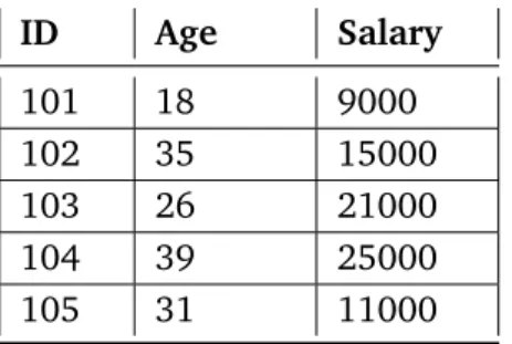
An overview of binary association rules is given in the previous section, where boolean values are used to represent the items. However, in reality, databases not only contain boolean attributes but also quantitative or categorical ones that cannot be mined using the classical technique. Identifying rules in such kind of data can be represented as the quantitative association rules problem [SA96]. To deal with quantitative attributes a possible approach is replacing them with several boolean attributes. It is straightforward to map quantitative attributes into binary values if they are categorical or if there are only a few values.

For example, the value of boolean field corresponding to(attribute1, value1)would be "1" ifattribute1hadvalue1in the original data, and "0" otherwise [SA96]. This only works if the original data has a very small number of values. It is required to split the values into intervals and map each attribute to the corresponding new boolean attribute when the number of different values increases. Now, to identify association rules, a binary algorithm can be used.

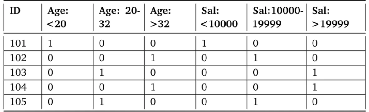
In Table 2.1, a sample database is shown. Here we can see that all the attributes are numeric so it is important to create intervals for all attributes. For each record of the table, an appropriate interval needs to be chosen. Then, each record is mapped to the corresponding new binary attribute. The number of columns in the new table is equal to the number of intervals chosen for each attribute. A mapping table with sample intervals chosen for each attribute is shown in Table 2.2.

ID Age: <20 Age: 20-32 Age: >32 Sal: <10000 Sal:10000-19999 Sal: >19999 101 1 0 0 1 0 0 102 0 0 1 0 1 0 103 0 1 0 0 0 1 104 0 0 1 0 0 1 105 0 1 0 0 1 0

Table 2.2:Mapping Table With this mapping method, two problems arise [SA96]:

• “MinSupport”: If the interval count for a single quantitative attribute is high, there could be a single interval which has low support. It is necessary to take larger intervals, otherwise, some existing rules containing this attribute may not be identified because they lack minimum support.

• “MinConfidence”: If a larger interval is taken in order to solve the first problem, another problem arises. The rate of information loss increases if the interval sizes become larger. Then, the appearance of determined rules might be different to the original data.

If the intervals are too large, it might not be possible to reach the minimum confidence, if they are too small, it might not be possible to achieve minimum support. The “MinSupport” problem can be solved by considering all potential continuous ranges over the ranges of the quantitative attribute. Increasing the number of intervals, without encountering the “MinSupport” problem, could be a solution for the “MinConfidenece” problem. By increasing the number of intervals and combining adjacent intervals simultaneously, creates two new problems:

• “ExecTime”: By using the above method, the number of items per record increases, so the execution time will increase as well.

• “ManyRules”: If a value has minimum support, any range that contains this value will also have minimum support. Hence, the number of rules will increase and many of them will not be interesting.

There is a trade-off between the above mentioned problems. If more intervals are built to cope with the “MinConfidence” problem, then execution time will increase and additionally, many rules might be generated which are not interesting.

2.1.4 Algorithms for Finding Association Rules

Since the introduction of the Apriori algorithm [AIS93], several algorithms have been developed. Those algorithms focus on the efficiency of finding a frequent pattern or

Figure 2.1:Representation of the itemsets [HGN00]

association rule identification. Apriori provides solutions for both problems. In this section, a brief overview of some important mining algorithms is given. Most of the algorithms work with binary association rules, but they also work with the quantitative association rules as well.

For developing an association rule mining algorithm there exist two main approaches, one is called breadth-first search (BFS) and depth-first search (DFS)[HGN00]. A lattice including all possible combinations of an itemset is shown in Figure 2.1.

The border between frequent and infrequent itemsets is represented by the bold line. All the items that lie above the border satisfy the minimum support requirements. The algorithms locate this border. In BFS, first, the support is computed for all itemsets in a specific level of depth, whereas DFS recursively subsides the structure by several depth levels. The algorithms for association rule mining can be systematized as depicted in Figure 2.2.

2.1.4.1 Apriori

The Apriori algorithm was the first developed algorithm for mining association rules out of a large dataset. It has been first introduced by Agrawal et al. [AS94]. The algorithm can find frequent patterns and generates association rules out of the frequent patterns.

Figure 2.2:Systematization of Algorithms [HGN00] k -itemset An Itemset having k items

Lk "Set of large k -itemsets (those with mini-mum support). Each member of this set has two fields: i) itemset and ii) support count."

Ck "Set of candidate k -itemsets (potentially large itemsets). Each member of this set has two fields: i) itemset and ii) support count. "

Table 2.3:Notation [AS94]

2.1.4.1.1 Discovering Frequent Itemsets A fact that is used to generate frequent item-sets is that any subset of large itemset must also be large as well. The size of an itemset is determined by the number of items contained in the itemset, an itemset is calledk−itemset

wherekis the size. The items in the itemset are stored in lexicographic order. The notation shown in Table 2.3 is used to represent the algorithm.

Each itemset associates a count field where the value of support is stored. Algorithm 2.1 shows the pseudocode of the Apriori algorithm. At first, the database is supplied for counting the occurrences of single elements. If the support value of a single element is below the minimum support that is defined by the user, it is not taken into consideration anymore. A subsequent pass k is composed of two phases:

• To generate the candidate itemsets,Ck for the current pass, the discovered large itemsets of pass k-1 , are used.

Algorithm 2.1Apriori algorithm Candidate Generation [AS94]

1: Fl=(Frequent itemsets of cardinality 1);

2: for(k= 1;Fk ̸=ϕ;k+ +)do

3: Ck+1= apriori-gen(Fk); // New Candidates

4: forall transactionst∈Databasedo

5: C_t′ =subset(Ck+1, t); // Candidates contained in t

6: forall candidates c∈C_t′ do

7: c.count++; 8: end for 9: Fk+1={C∈Ck+1|c.count≥minimumsupport}; 10: end for 11: end for 12: Answer∪_kFk

• The database is searched again determining the support for the candidate itemsetsCk. The candidates which have a support above the minimum support will be included to the large itemsets. To prevent a long counting duration, identifying the right candidates is important.

The functionapriori-genshown in Algorithm 2.1 takes the itemsets of the previous iteration as an input. These itemsets are joined together, composing itemsets with one more item than in the previous step. Then in the prune step, those itemsets will be removed whose sub-combinations have not been part of the discovered sets in previous iterations. A hash-tree is used to store the candidate sets. This hash-tree can either have a list of itemsets, called a leaf node, or a hash table, which is called an interior node.

The functionsubsetstarts traversing the hash-tree from the root node and traverses until the leaf nodes for finding all candidates that are in a transactiont. The function will ignore the itemsets which start with an item that is not int.

2.1.4.1.2 Discovering Association Rules Association rules can have multiple elements in the antecedent and also in the consequent. To generate the association rules, only large itemsets are used. The first step of the procedure is to find all possible subsets of the large itemsetl. A rule is defined in the forma → (l−a) for each of those identified subsets. If the confidence of the rule is greater than the user-defined minimum confidence, then the rule is considered as interesting. All subsets oflare discovered so that any possible dependencies are not missed. The algorithm for generating association rules is shown in Algorithm 2.2.

2.1.4.2 Frequent Pattern Growth (FP-Growth)

The FP-Growth algorithm generates frequent itemsets. It tries to avoid generating a large candidate set like the Apriori algorithm. The basis of this algorithm is a solid representation

Algorithm 2.2Apriori algorithm Association Rule Generation [YKTZ11]

1: for each frequent itemsetsik (k≥) do

2: H1={h∈lk}|cf(lk− {h} ⇒ {h})≥min_cf 3: CallAp-GENRULE(lk, H1); 4: end for 5: procedure AP-GENRULE(lk, Hm ) 6: ifk > m+ 1then 7: Hm+1 =apriori_gen(Hm); 8: for allhm+1 ∈Hm+1 do 9: cf =sp(lk)/sp(lk−hm+1) 10: ifcf ≥min_cf then 11: elseHm+1:=Hm+1− {hm+1}; 12: end if 13: Ap-GENRULE(lk, Hm+1); 14: end for 15: end if 16: end procedure

of the original data set without losing any information. This is done by constructing a tree, using the data. This tree is called the Frequent Pattern Tree, FP-Tree in short. The FP-Growth algorithm has been introduced in [HPY99]. Here, the FP-Tree is constructed out of the original data set first, and then the frequent patterns are generated from the tree. Before applying the algorithm, the data should be preprocessed in order to minimize the execution time.

2.1.4.2.1 Preprocessing the Data The FP-Growth algorithm applies following prepro-cessing steps for efficiency [Bor05]:

• First, the initial dataset is scanned and for each item, the support is calculated. Then, all items that have a support below the user defined minimum support are discarded from the transactions.

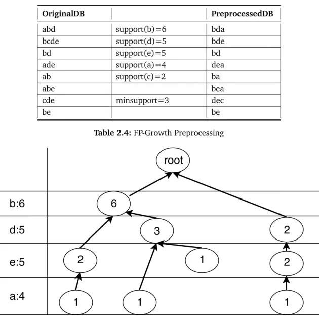
• The remaining items are stored in a decreasing order according to their support. Although, the algorithm works fine without sorting, it works much faster after sorting [Bor05]. If increasing order is used instead of decreasing order, it performs worse than using a random order [Bor05]. Table 2.4 provides an example of preprocessing steps for a transaction of the FP-Growth algorithm.

2.1.4.2.2 Constructing the FP-Tree An FP-Tree can be constructed out of the prepro-cessed data. A scan over the database is done for adding each itemset to the tree. The first branch of the tree will be the first itemset. In case of the transaction shown in Table 2.4, the itemsb,dand a would be the first branch. The second transaction has the prefixbd which already exists in a set of the tree. In this case, the count of each node along the path

OriginalDB PreprocessedDB

abd support(b)=6 bda

bcde support(d)=5 bde

bd support(e)=5 bd

ade support(a)=4 dea

ab support(c)=2 ba

abe bea

cde minsupport=3 dec

be be

Table 2.4:FP-Growth Preprocessing

Figure 2.3:FP-Tree [HGN00]

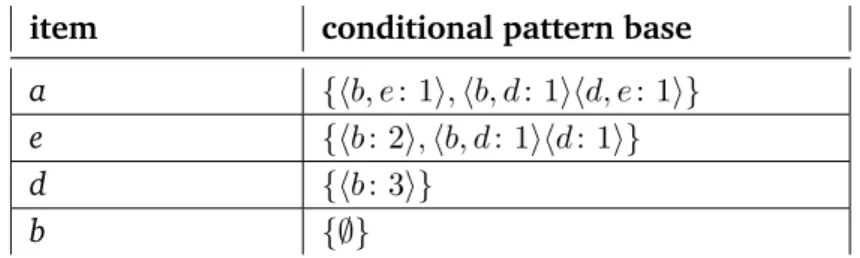
of the common prefix is increased by one, and for the remaining items, new nodes will be created and linked as a child. In case of the example shown in Table 2.4, only a new node forewill be created and linked as a child ofd. For the transaction database of Table 2.4, the generated tree is shown in Figure 2.3. It represents the database without losing any information.

Each node of the FP-Tree has three fields [HPY99]:

• item-name: The name of the item representing the node is stored in this field. • count: The accumulated support of the node within the current path is represented

item conditional pattern base a {⟨b, e: 1⟩,⟨b, d: 1⟩⟨d, e: 1⟩} e {⟨b: 2⟩,⟨b, d: 1⟩⟨d: 1⟩}

d {⟨b: 3⟩}

b {∅}

Table 2.5:Conditional Pattern Bases

• node-link: It represents the link between the nodes. It stores the ancestor of the current node, and null in case there is none.

After building the FP-Tree, the database is not required anymore for mining. Now the FP-Tree can be used. The support of an itemset can easily be calculated by traversing the path and using the minimum value of count from the nodes. For example, the support of itemset{b, e}will be 2 and the support of itemset{b, e, a}will be 1.

2.1.4.2.3 Mining the FP-Tree using FP-Growth The FP-Tree provides an efficient struc-ture for mining, however one may still encounter the combinatorial problem of candidate generation which needs to be solved. For identifying all frequent itemsets, the FP-Growth algorithm takes a look at each level of depth of the tree [PEl16]. It starts from the bottom and generates all possible itemsets that include nodes in that specific level. After generating frequent patterns for each level, they are stored in the complete set of frequent patterns. The procedure of the algorithm is shown in Algorithm 2.3.

The algorithm is executed at each of these levels. The tree is first checked for the number of paths it contains for finding all the itemsets containing a level of depth. If the tree is a single path tree, all possible combinations of the items contained in it will be generated [PEl16]. Then, these will be added to the frequent itemsets.

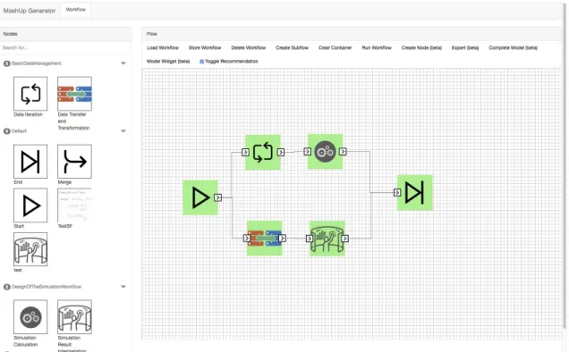
If the tree has more than one path, then for the specific depth, a conditional pattern is constructed. In FP-Tree of Figure 2.3, for the depth levela, the conditional pattern base will consist of the following itemsets : ⟨b, e: 1⟩,⟨b, d: 1⟩and ⟨d, e : 1⟩. The item set is determined by traversing each path in an upward direction. The conditional pattern for all depth levels of the tree is shown in Table 2.5.

From the conditional pattern base, a conditional FP-Tree is built. This is done in the same way as the construction of the initial tree. The only difference is now that, the conditional pattern base is used instead of a transactional database. After having the conditional FP-Tree, the FP-Growth function is called recursively. This is done until the tree has only a single path or it is empty. At the end, all the items in the various condition FP-Tree are stored. Then, these items are returned as a list of frequent itemsets in the FP-Tree as well as in the database, respectively.

Algorithm 2.3FP-Growth algorithm [HPY99] procedureF(P)-Growth (T ree, α)

ifTree contains a single pathP then

forall combination (denoted asβ ) of the nodes in the pathP do

generate patternβ∪αwith support = minimum support of nodes inβ; end for

forallai in the header ofT ree do

generate patternβ =ai∪αwith support=ai. support ;

constructβ’s conditional pattern base and thenβ’s conditional FP-TreeT reeβ; if T reeβ ̸=∅then

call FP-growth(T reeβ,β) end if

end for end if end procedure

2.2 FlexMash

In recent times, the data processing and integration is becoming complex because of an increasing size of IT systems used in enterprises and a growing connectivity between the corresponding data sources. This leads to high communication effort between domain-specific users, such as business persons and IT experts who implement the data processing. In most cases, this result in non-flexible solutions that work only for specific use cases. To solve this issues, a solution is required that allows users to define data processing and integration scenarios without defining any execution details.

Mashup plans that were introduced by Hirmer et al. [HRWM15], are graph-based models that enable domain-specific modeling of data mashups. Based on this Mashup plan, an approach named FlexMash is introduced by Hirmer et al. [HM16] that allows modeling and pattern based execution of data mashups. This tool transforms the Mashup Plans into an executable solution based on requirements defined by the use case scenario. Figure 2.4 shows a high-level view of the FlexMash tool.

First of all, a modeling of the Mashup Plan is required that describes the processing and integration of data. Then, a pattern is selected by the user that defines the requirements for mashup execution. Based on this selected pattern, the defined Mashup plan is transformed into an executable representation. Finally, the executable representation is executed in a suitable engine. It is possible to store and visualize the result of execution for later use. This tool enables a flexible solution for data mashup execution that is specific to user requirements and uses transformation patterns selected by the user. Figure 2.4 shows a screen shot of the FlexMash application.

Rodríguez et al. [RCD+14] introduced an approach named Assisted Mashup Development. In this work, they use Yahoo! Pipes, a web-based mashup editor, as a mashup model development tool. They aim to assist users by recommending development knowledge. By mining existing mashup models, a set of composition patterns is discovered. These composition patterns are then interactively recommended to the users during mashup development. A canonical mashup model is described that is able to formalize different data flow mashup languages into a single modeling formalism. A set of composition patterns is then extracted out of this canonical mashup model. For each of the discovered patterns, a respective pattern mining algorithm is implemented that discovers the composition knowledge as reusable mashup patterns out of the stored mashup models. Finally, these patterns are recommended to the users based on the user actions on the modeling canvas. An automatic weaving of recommended patterns is also included. In this approach, they focus on how to automatically discover patterns from existing mashup models, recommend the discovered patterns fastly to the users, and automatically weave the recommended patterns into mashup models.

The goal of this thesis is to assist users to define a mashup plan for execution in the FlexMash environment. A set of transformation patterns is already introduced in FlexMash which users can select during the design of the model as a node. All data sources and operations are represented as nodes in FlexMash. The user can select data sources as well as operations from the node catalog. So pattern selection is out of the scope of this thesis. Instead of implementing a separate algorithm for each pattern, a common mining algorithm is used in this work which recommends the frequently used nodes together. It happen that, the Mashup modeler is a business user who does not have technical knowledge which nodes to model. In that case, the models that have been executed successfully in past can be analyzed to recommend the users which node or pattern to use. A canonical model is used to convert different models into a single modeling structure. Based on this canonical model, a data mining algorithm is used to generate the recommendation. The model designed in FlexMash is captured by the recommendation application during execution and converted into the canonical model. The Assisted Mashup Development approaches do focus on recommendation of composition patterns. They discover a set of composition patterns and design separate mining algorithms for each discovered pattern. However, the aim of this thesis is not only recommending the patterns but also the data sources that have been used previously. The work done in this thesis also provides an interactive recommendation feature. The difference is that, it is not only recommending nodes but also automatically completes the whole model using the top recommended nodes. So the user does not always need to have modeling knowledge. In addition, it also has a modeling

widget feature which can be used to design a partial model using the recommendation feature and weave this partial model into the main model in the modeling canvas. The recommendation is updated each time a mashup model is executed.

Roy Chowdhury at el. [CRDC12] introduced Baya, an extension of Yahoo! Pipes, for speeding up development by interactively recommending composition knowledge. It has two parts: one is the Baya recommendation server and the other is the Baya Firefox extension. The Baya recommendation server first takes the native models designed in the mashup tool and converts them into a canonical mashup model which is able to describe a different kind of similar mashup languages in a generic manner. Then a pattern miner runs a set of pattern mining algorithms on the canonical model to discover a set of patterns. Currently, Baya supports the following composition patterns: Parameter value pattern, Connector pattern, Connector co-occurrence pattern, Component co-occurrence pattern, Component embedding pattern, Multi-component pattern. These discovered patterns are stored in a canonical pattern database. A data transformer transforms and stores them into a persistent knowledge base. The Baya Firefox extension is composed of two main components: a recommendation engine and a pattern weaver. The recommendation engine communicates between client and recommendation server. The pattern weaver weaves the selected recommendation into a partial mashup model in the modeling canvas. After weaving of a pattern from recommendation, the knowledge base is updated. This updated metadata again is used for future recommendation.

In contrast to their work, the main focus of this thesis is modeling node recommendations in pattern-based mashup environments where a set of transformation patterns is already defined and represented as a node in a node catalog with other data source nodes. This thesis offers a recommendation of frequently co-occurred nodes together because both patterns and data sources are represented as a node in FlexMash. So there is no need to capture modeling actions that occurred in the modeling canvas. In addition, an interactive recommendation feature is offered in this thesis which is not present in the work of Roy Chowdhury at el. The system not only recommends the nodes but also places the node in the modeling canvas upon user selection. It also offers a modeling widget for designing a partial model and users can also toggle the recommendations.

Roy Chowdhury at el. [CTN+13] introduced an approach OMELETTE, a hybrid devel-opment assistance system. The system is developed on top of the open source mashup platform Apache Rave. It has two parts: the Automatic Composition Engine (ACE) which addresses users who have no or very little knowledge in mashup development and the Pattern Recommender (PR) which targets users who are already familiar with the com-position environment. The ACE helps users to specify their goals using a dialog-based interface in an interactive manner. The dialog shows up in a question-answer manner out of which the system refines user goals. It helps users to choose and configure widgets out of a large collection of potentially incompatible components in an interactive way. The PR helps users by recommending existing composition knowledge stored in a knowledge base (KB). Currently, it supports two composition pattern types: widget co-occurrence and multi-widget patterns. Based on user modeling actions on widgets, the PR reacts during composition. The recommendation engine uses an event listener to capture the modeling

on current composition context and are rendered in the recommendation panel. The user can select recommended patterns from the recommendation panel and upon selection of a pattern, the PR applies the pattern to the current workspace model automatically.

In this thesis, the main goal is to recommend possible nodes that are used frequently by the users for each node that is placed in the modeling canvas. For each placed node, users can see the recommendations by calling the recommendation dialog. The recommendation ap-plication recommends the nodes used frequently with the placed nodes based on association rules techniques. The recommendations are ranked based on the confidence level. Upon user selection, the selected node from the recommendation dialog is automatically placed in the modeling canvas and connected to the placed node. The main key difference with their approach is that they recommend composition patterns of a widget of Apache Rave whereas the approach, proposed in this thesis, recommends the frequently co-occurred nodes because patterns are represented as nodes in FlexMash. Another key difference is that a good interactive recommendation feature is provided which recommends nodes at each step of modeling based on user selection. It also automatically completes the whole model using top recommended nodes from the recommendation server.

Roy Chowdhury at el. [RDC11] proposed an approach for efficient and faster retrieval of a ranked list of development recommendations. They model the problem of interactively recommending composition knowledge as pattern matching and the retrieval problem in the context of data mashups and visual modeling tools. They propose a solution for the problem of matching a partial mashup model with a repository of composition patterns. In order to achieve this, they transform the graph-like data structure into an optimized structure which is directly mapped to the recommendations to be provided. They also have an efficient similarity search algorithm for complex pattern matching with the recommended pattern repositories.

In this thesis, the models designed in FlexMash are transformed into a canonical model. This canonical model stores the information about each connection of the model supplied by FlexMash. A data mining process is applied to this canonical model to generate association rules. Each association rule is a connection that occurred frequently in the repository of canonical models. In this approach, a unique id of each node is provided by FlexMash which is used to retrieve the recommended nodes from the repository of association rules.

Pattern-based Mashup Plans

In this chapter, the overall architecture of the master thesis, the different components that were developed in order to extend the FlexMash application with recommendation facilities is described. The architecture of the recommendation application and how to integrate it with the existing FlexMash application are also explained in detail.

Through the development of this thesis, an application for generating recommendations is developed which includes a set of services. This set contains services for processing and storing data that comes from FlexMash and for generating recommendations. It is important to highlight that the application is centralized and all models that are executed by any instance of FlexMash will be captured by the application in order to do the analysis for recommendation generation.

4.1 Overview of the approach

In this section, the overall approach to achieve the goal of the thesis is described. In order to assist users by recommending nodes during modeling, the FlexMash application needed to be extended to make it compatible with the recommendation application. Furthermore, for designing the recommendation application, the underlying canonical model and an appropriate mining algorithm have to be defined.

After developing the recommendation application, it needs to be adjusted with FlexMash to get recommendations during modeling. The work done in this thesis consists of:

• Creation of the training data, i.e., the flow models from FlexMash. • Creation of the underlying canonical model for analysis.

• Analysis and selection of a suitable analytics algorithm to generate the recommenda-tions.

• Design of the repository for storing the canonical model and the generated recom-mendations.

• Design of a data transformer that transforms the flow models supplied by FlexMash to the canonical model.

Figure 4.1:Overall Approach of the Thesis

• Integration into FlexMash in order to enable the interactive recommendation feature. Figure 4.1 shows an overview of the approach. The whole approach is subdivided into four steps: (i) Creation of the mashup plan, (ii) Creation of an underlying canonical model, transformation of the mashup plan and storing, (iii) Algorithm selection, analysis and storage of results, and (iv) integration with FlexMash.

4.2 Step 1: Creation of the mashup plan

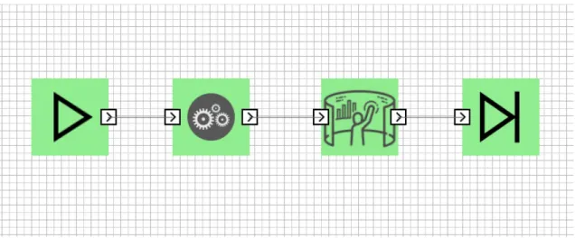
The first step, the creation of mashup plans is already done in the existing FlexMash application. Users can model a mashup plan in FlexMash that defines data as well as how it is processed and integrated. After that, the mashup plan is executed. The model is sent to the recommendation application during the execution. Each model that is executed in FlexMash will be captured by the recommendation application for analysis. A model designed in FlexMash is shown in Figure 4.2. In the next step, a canonical model needs to be defined and the model needs to be transformed into the defined canonical model.

4.3 Step 2: Creation of underlying canonical model and

transformation

To generate recommendations, a canonical model is needed which contains only basic and unique information about the models generated by FlexMash. In the model that is shown in Figure 4.2, each node is connected with others by a connection. So each connection has a source node and a target node. As already mentioned, in this thesis, association rules technique is used to generate recommendation. The basic idea behind association rules is to identify frequent patterns as already discussed in Section 2.1. How frequently one node is used with others can be found by storing the connections between nodes used in each model that is sent from FlexMash.

The canonical model used in this work for analysis can be expressed as a tuple

m=⟨id, sourceId, targetId⟩where :

• idis the connection id which will be auto generated,

• sourceIdis the id of the source node which is a unique id of the node in FlexMash. • targetIdis the unique id of the target node.

The mashup model sent by FlexMash needs to be transformed into this canonical model. Each tuple in the canonical model can be considered as a transaction for association rules analysis.

4.3.1 Transform

The transformation is done using the JSON format that is sent by the FlexMash application to the canonical model introduced in the previous section. The JSON format is depicted in Listing 4.1.

After executing the designed model, the JSON representation of the model is sent from the FlexMash application through HTTP. The JSON data sent by FlexMash contains the id of the nodes and the connections between nodes. The recommendation application extracts the relevant data from the file in order to transform it into the canonical model. For the transformation, the unique id of the nodes in the model and connections between the nodes are needed. The other data is ignored since it is not needed.

The model depicted in Listing 4.1 can be represented using the following mathematical construct:

M =⟨Nx, Ny, Nz⟩

{ "Nodes": [ { "guiId":"4c7c775e-5922-463e-8f80-9719e9b8d5da", "serviceId":"849AFDC4-45A1-3700-AB70-2A32E650C9EA", "Properties":[], "Target": [ "b7e3465d-f12d-490c-adef-d3a3036a22fa", "b868a562-f84c-414a-85f3-f359c4449c95" ] }, { "guiId":"b7e3465d-f12d-490c-adef-d3a3036a22fa", "serviceId":"3601AFC0-13B3-2BA7-B428-747F02A8BD89", "Properties":[], "Target": [] }, { "guiId":"b868a562-f84c-414a-85f3-f359c4449c95", "serviceId":"5AE4C8CA-D491-224F-A78C-4578F69896AF", "Properties":[], "Target": [] } ], "Identifier":"6f2e2a9f-2b74-462c-9503-8608db791c4b" }

Listing 4.1:JSON Representation of the Model Each node of the model can be represented as:

Nx=⟨gx, sx, Px, Tx⟩

Where,gx is theguiId,sxis theserviceId,Pxrepresents thePropertiesandTx is the list of Targetnodes in the model for the nodeNx. And

Tx =⟨gy, gz⟩,

where,gy andgz is theguiIdof target nodes of the source nodeNx. The other nodes in the model can be represented as follows:

Ny =⟨gy, sy, Py, Ty⟩andTy =∅,

Nz=⟨gz, sz, Pz, Tz⟩andTz =∅.

To transform the FlexMash model into the canonical model we need onlyguiId,serviceId andTargetof each node, thePropertiescan be discarded as it is not needed for our canonical model defined in Section 4.3.

Let, first consider the nodeNx. Thesx is theserviceIdof the nodeNxwhich is the unique id of this node in FlexMash. The target nodes of the nodeNx aregy andgz, wheregy and

Algorithm 4.1Algorithm for Transformation

1: N odes=Parse JSON array of Nodes;

2: for(i= 1;i≥N odes.length;i+ +)do

3: sourceID =N odes[i]["serviceID"];

4: Targets =N odes[i]["target"];

5: for(k= 1;k≥T argets.length;k+ +)do

6: initializeconnectionobject;

7: set sourceID asconnectionsource;

8: map Targets[k]["guiID"] toN odes[i]["serviceID"];

9: setconnectiontarget;

10: end for

11: end for

gz are theguiIdof the nodeNy andNz, respectively. So, there are two connections, one between nodeNx andNy, and the other betweenNxandNz.

The canonical model contains tuples of connections in the model and is represented as:

m=⟨id, sourceID, targetID⟩

So, the above mentioned mathematical representation of the model can be transformed into the canonical model as follows:

m1 =⟨id, sx, sy⟩,

m2 =⟨id, sx, sz⟩

Where,idis the unique identifier for the connectionm1,sxis theserviceIdof the nodeNx andsy is theserviceIdof the nodeNy. For connectionm2,sx is theserviceIdof nodeNx andszis theserviceIdof the nodeNz.

The nodes Ny and Nz have no target nodes, so these are the end nodes. There are no outgoing connections from these nodes, so we do not have to transform these nodes. Algorithm 4.1 outlines the approach for model transformation. Here, first the JSON array is parsed and added intoNodes. Then, by iterating over all items of theNodesarray, the source and the target of a connection are extracted.

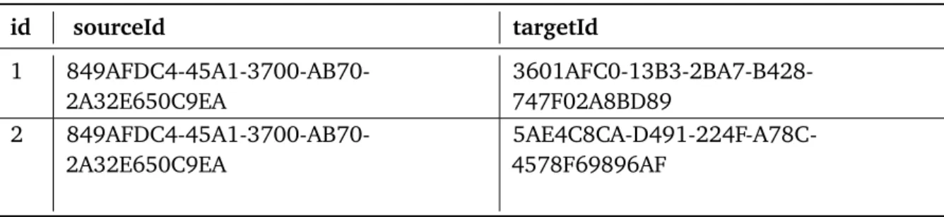
id sourceId targetId 1 849AFDC4-45A1-3700-AB70-2A32E650C9EA 3601AFC0-13B3-2BA7-B428-747F02A8BD89 2 849AFDC4-45A1-3700-AB70-2A32E650C9EA 5AE4C8CA-D491-224F-A78C-4578F69896AF

Table 4.1:Database Table Structure with Example Records to Store Canonical Models

4.3.2 Store

The above mentioned canonical model needs to be stored in a relational database. The design of the relational database used in this work is discussed in Section 5.3 in detail. All models coming from FlexMash are transformed into the canonical model and are stored in a table of a relational database. The analysis is done based on this table. Each time a model is executed in FlexMash, it is captured by the recommendation application, transformed into the canonical model and stored in the database. The analysis is run on all data stored in the canonical model table and updates the result of the analysis. Table 4.1 shows the structure of the database table with some example canonical model records to store the canonical models.

Next, a suitable algorithm needs to be selected for association rules analysis.

4.4 Step 3: Algorithm selection for analysis

In this section, the selection of a suitable algorithm for association rules analysis is discussed. The algorithms discussed in Section 2.1.4 are compared based on several parameters. Based on this performance comparison, a suitable algorithm is selected for analysis.

There are two disadvantages of the Apriori algorithm that has been discussed in Sec-tion 2.1.4.1. One is the complex process of candidate generaSec-tion that uses most of the time, space, and memory. Another disadvantage are the multiple scans of the database. FP-Growth solves these two disadvantages of Apriori. FP-FP-Growth generates frequent itemsets with only two passes over the database and without any candidate generation process. By doing so, it solves one disadvantage of the apriori algorithm. In FP-Growth, the frequent patterns generation consists of two sub-processes: construction of FP-Tree, and generation of frequent patterns from the FP-Tree.

The FP-Growth algorithm is efficient because of three reasons. First, the FP-Tree constructed by the algorithm is the compressed representation of the actual database because only frequent items are used to generate the tree, other irrelevant data are discarded. Also, the overlapping parts appear only once with different support count by ordering the items according to their supports. Secondly, this algorithm scans the database only twice. The

generated FP-Tree contains patterns with the specified suffix from which frequent patterns can be easily generated. Also, the cost of computation decreases. Third, The FP-Tree uses a divide and conquer method which reduces the size of the subsequent conditional FP-Tree. In data mining, one critical aspect is the number of disk accesses because the I/O operation takes more time than the memory operation. So, minimizing the disk access can be a reason for faster execution. The Apriori algorithm scans the whole database k-times for finding k-frequent itemset. The number of times the algorithm reads the database is dependent on the size of the longest itemset. In contrast, the FP-Tree algorithm scans the database only twice.

However, FP-Growth is difficult to use in an interactive mining system. In the interactive mining process, users may change the threshold of the support according to the rules. In case of FP-Growth, if the user changes the threshold of the support, the whole mining process will be repeated. FP-Growth is also not suitable for incremental mining. Since

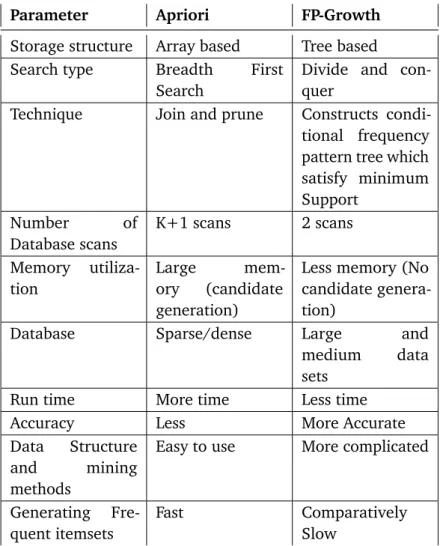
Parameter Apriori FP-Growth

Storage structure Array based Tree based Search type Breadth First

Search

Divide and con-quer

Technique Join and prune Constructs condi-tional frequency pattern tree which satisfy minimum Support Number of Database scans K+1 scans 2 scans Memory utiliza-tion Large mem-ory (candidate generation)

Less memory (No candidate genera-tion)

Database Sparse/dense Large and

medium data

sets

Run time More time Less time

Accuracy Less More Accurate

Data Structure

and mining

methods

Easy to use More complicated

Generating Fre-quent itemsets

Fast Comparatively

Slow

databases keep growing, new datasets may be added into the database. The whole process may repeat because of those additions, in case the FP-Tree algorithm is used.

Table 4.2 summarizes the difference between Apriori and FP-Growth based on literature review [SS13].

4.4.1 Experimental Evaluation

I tested the performance of the Apriori and FP-Growth algorithms in Weka1. Weka is an open source software that consists of a collection of open source machine learning and data mining algorithms. It also includes preprocessing of data, classification, clustering, and association rule extraction. The performance evaluation of both algorithms is done based on execution time. I used supermarket data included in Weka as sample data. The execution time is measured for the different number of records, support and confidence level. For efficiency evaluation, I used GUI based WEKA application.

4.4.1.1 Result Discussion

In this section, the result of the experimental evaluation done for both Apriori and FP-Growth is discussed.

Table 4.3 shows the result of the execution time analysis of Apriori and FP-Growth for a different number of instances. It can be seen that the execution time of both algorithms decreases when the number of instances decreases. Apriori takes 48 seconds when the number of instances is 3629. For the same number of instances, FP-Growth needs only 4 seconds for constructing association rules.

In Figure 4.3, the performance of Apriori and FP-Growth is compared based on execution time. Each algorithm is executed on different data sets with sizes of 3629, 1688 and 942. Here, the number of instances in the dataset is represented by the x-axis and execution time is represented by the y-axis. The figure shows that for any number of instances the execution time of the FP-Growth algorithm is less than the Apriori. So, the FP-Growth

Number of instances Execution Time(in seconds) Apriori FP-Growth

3629 48 4

1688 26 3

942 8 2

Table 4.3:Execution Time for Different Number Of Instances

Figure 4.3:Comparison of Execution Time Based on Number of Instances executes faster than Apriori.

Table 4.4 shows the execution time taken by both Apriori and FP-Growth for different confidence levels. The execution time of both algorithms is high when the confidence level

Confidence Execution Time(in seconds) Apriori FP-Growth

0.5 16 2

0.7 19 3

0.9 57 4

Table 4.4:Execution Time for Different Confidence Level

is high. When the confidence level is 0.9, Apriori takes 57 seconds and FP-Growth takes 4 seconds to generate association rules.

Figure 4.4 shows the graphical representation of the relationship between time and confi-dence. The confidence is represented by the x-axis and execution time is represented by the y-axis. It shows that the execution time of FP-Growth is less than the Apriori for any confidence.

From the above discussion and result analysis, it is proven that FP-Growth performs faster than Apriori. However, for providing a flexible solution, in this thesis, both algorithms are used for analysis and results of this analysis is stored separately. The users can select which algorithm to use according to their use case.

4.4.2 Analysis

In this section, the Apriori algorithm is used to generate association rules from the canonical models stored in the database. An example canonical model instance is shown in Table 4.5. This table represents a model designed in FlexMash.

As already discussed in Section 2.1.4.1, the Apriori algorithm has two steps: (i) Frequent itemsets generation, and (ii) Association rules generation using the frequent itemset.

id sourceId targetId 1 849AFDC4-45A1-3700-AB70-2A32E650C9EA 5AE4C8CA-D491-224F-A78C-4578F69896AF 2 5AE4C8CA-D491-224F-A78C-4578F69896AF B4652E72-1F34-69D5-BC35-6AEDA218B0C5 3 B4652E72-1F34-69D5-BC35-6AEDA218B0C5 A203915A-39C0-7CF1-92F6-81B6A42C4BF4 4 A203915A-39C0-7CF1-92F6-81B6A42C4BF4 DDCB56F7-D526-E011-936C-177094DDA67B

Item Sup. Count 9EA 1/4 6AF 2/4 0C5 2/4 BF4 2/4 67B 1/4 Itemset Sup. Count {9EA, 6AF} 1/4 {9EA, 0C5} 0 {9EA, BF4} 0 {9EA, 67B} 0 {6AF, 0C5} 1/4 {6AF, BF4} 0 {6AF, 67B} 0 {0C5, BF4} 1/4 {0C5, 67B} 0 {BF4, 67B} 1/4

Itemset Sup. Count

{9EA, 6AF} 1/4 {6AF, 0C5} 1/4 {0C5, BF4} 1/4 {BF4, 67B} 1/4 Frequent 1-itemsets Frequent 2-itemsets L1 1st scan 2nd scan Item Sup. Count 9EA 1/4 6AF 2/4 0C5 2/4 BF4 2/4 67B 1/4 L2

Figure 4.5:Frequent Itemset Generation

4.4.2.0.1 Frequent Itemsets Generation The data represented in Table 4.5 is consid-ered as transactional data to generate frequent itemsets using Apriori. Here, four con-nections are represented. I assume that, the minimum support is 25% (i.e. 1/4) and the confidence is 40%.

A high-level illustration of the frequent itemset generation using Apriori is depicted in Figure 4.5. Here, the last three digits of nodeID are used to represent the nodes. At first, each node is considered as a frequent 1-itemset. Then, the support is calculated for each item in the transactions. The support is calculated using the following formula :

support(9EA)= transactions_containing_node_9EA

total_number_of_transactions

In L1, the overall support count is above the minimum support (25% i.e. 1/4), so all items can be considered for the next iteration. In the next iteration, to generate frequent 2-itemsets, the Apriori algorithm uses L1 Join L1. Then, the support count for each itemset is calculated which is shown in the third table of Figure 4.5. After that, the set of frequent 2-itemsets, L2, is determined by discarding the items which have a support count below minimum support. The itemsets shown in table L2 of Figure 4.5 are the frequent itemsets which can be used to generate association rules.

4.4.2.0.2 Generating Association Rules To generate association rules from frequent itemsets, for each frequent itemset, the confidence is calculated. The formula for calculating the confidence is given below:

Association Rules Support(A,B) Support(A) Confidence

9EA→6AF 1/4 1/4 1

6AF →0C5 1/4 2/4 1/2

0C5→BF4 1/4 2/4 1/2

BF4→67B 1/4 1/4 1

Table 4.6:Generated Association Rules out of Frequent itemsets

confidence(A→B) = number_of_transactions_containing_both_A_and_B

number_of_transaction_containing_A

The generated association rules are shown in Table 4.6. As all rules have confidence level above minimum confidence, all rules can be considered.

4.5 Step 4: Integration with FlexMash

One of the main goals of this thesis is to assist users in the FlexMash application by providing modeling recommendations. In order to achieve this goal, the recommendation service needs to be integrated into the existing FlexMash application. Figure 4.6 shows how the integration is done between the Recommendation service and the FlexMash application.

In the first step, the model designed in FlexMash is sent to the Recommendation Service during the execution of the model. The Recommendation Service has a component which transforms the model into a canonical model. This canonical model is then stored in the repository. The analysis process will use all the stored canonical models for generating association rules. Then, the result of the analysis are stored in the repository. This model transformation and analysis is done during each execution of the model in FlexMash. After that, FlexMash can query for recommendations for a specific node. The Recommendation Service sends all available association rules for this specific node to FlexMash.

A set of User Interfaces needs to be implemented inside FlexMash in order to provide an interactive recommendation feature during modeling.

The implementation details of this thesis work are discussed in this chapter which includes the approach discussed in the previous chapter. To generate recommendations by analyzing existing models, a web service namedModeling Recommendation Serviceis implemented. The chapter describes how to transform the models into a canonical model, how the analysis process is done and how the service is integrated into FlexMash. This chapter also outlines the required user interface implementation in the FlexMash frontend in order to achieve the interactive recommendation feature. FlexMash is an open source application so the work done in this thesis is also open source.

5.1 Adaptation of Technologies

The section states the technologies needed for the implementation of the recommendation service.

• Node.js : The Recommendation service implemented for this thesis is developed in Node.js which is a JavaScript runtime built on Chrome’s V8 JavaScript engine.It is lightweight and efficient because it uses an event-driven, non-blocking I/O model. Node.js allows the creation of Web servers and networking tools using JavaScript and a collection of "modules" that handle various core functionalities. Node.js applications can run on Linux, MacOS, Microsoft Windows and Unix servers.

• JAVA : The data mining process in this work is implemented in JAVA which is a concurrent, class-based object-oriented programing language. JAVA is used to handle the open source library Weka which consists of a collection of machine learning algorithms for data mining tasks.

• MySQL:The repository used in this work for storing canonical models and analysis results is implemented in MySQL. It is one of the most popular relational database management systems.

• TypeScript: The FlexMash application is implemented in TypeScript which is an open source programing language developed and maintained by Microsoft. TypeScript is a superset of JavaScript.

Figure 5.1:Architecture of theModeling Recommendation ServiceSpecific to the Implemen-tation Scenario

• HTML/CSS/jQuery : This thesis uses HTML and CSS to implement additional user interfaces inside FlexMash for the interactive recommendation feature. Along with these, this thesis also uses libraries like Bootstrap, jQuery, etc.

5.2 Architecture

This section gives an insight into implementation details. An overview of the architecture specific to the implementation for the work done in this thesis is depicted in Figure 5.1. TheModeling Recommendation Serviceis hosted as a web service. It can be easily accessed, deployed, and scaled.

The Architecture of theModeling Recommendation Serviceconsists of two main processes. First, the Model Transformer, that transforms the model sent by the FlexMash application into a canonical model and stores it into the database. Second, the Data Mining Process which includes two subprocesses: (i) Transform canonical models into the Attribute-Relation File Format (ARFF) [wik], and (ii) the Mining process that mines the supplied ARFF dataset using the data mining algorithms Apriori and FP-Growth. The result of the data mining process (association rules) is stored in the database.

The database consists of two core models : (i) Canonical models, (ii) Association Rules. The database is described in more detail in Section 5.3.