VCU Scholars Compass
Theses and Dissertations Graduate School
2008
Probe Level Analysis of Affymetrix Microarray
Data
Richard Ellis Kennedy
Virginia Commonwealth UniversityFollow this and additional works at:http://scholarscompass.vcu.edu/etd Part of theBiostatistics Commons
© The Author
This Dissertation is brought to you for free and open access by the Graduate School at VCU Scholars Compass. It has been accepted for inclusion in Theses and Dissertations by an authorized administrator of VCU Scholars Compass. For more information, please [email protected].
Downloaded from
A dissertation submitted in partial fulfillment of the requirements for the degree of Doctor of Philosophy at Virginia Commonwealth University.
by Richard Ellis Kennedy
Bachelor of Arts in Computer Science, 1990 University of Mississippi, Oxford, Mississippi
Doctor of Medicine, 1994
University of Mississippi Medical Center, Jackson, Mississippi
Director: Kellie J. Archer, Ph.D. Assistant Professor Department of Biostatistics
Virginia Commonwealth University Richmond, Virginia
Acknowledgements
A project of this magnitude represents the culmination of many months of effort, but repre-sents only a small portion of my time in graduate school. In the past six years, I have met many new friends, begun a new career, matured in my marriage, and seen the birth of my two children. I am grateful to all of the people who have made this experience so rich and rewarding.
My advisor, Dr. Kellie Archer, has been a wonderful mentor during my studies and the com-pletion of my dissertation. Her intellectual curiosity and breadth of knowledge was, and will continue to be, an excellent example for me to follow in my own work. She has also been stead-fastly supportive of my pursuits and a source of encouragement during the difficult times that are a part of graduate school. Without her guidance, this dissertation would still be just an interesting idea that I had come across during the course of my studies.
My remaining committee members have also been excellent. Dr. Ramesh has never ceased to give of his time, both inside and outside of the classroom, to help with my learning; he is a teacher in the truest sense of the word. Dr. Best has always provided a sharp eye for details, and my dissertation would not be nearly so polished and eloquent without his involvement. Dr. Miles and Dr. Zhao have both ensured that I have a good understanding of the biological principles that are so critical to work in this area of biostatistics. I thank you all for your influence on my education and my career.
All of this would not have been possible without the support of my family through the years. My mother and father instilled a lifelong commitment to learning through their example and made sure that ample educational opportunities were available to me. It is only now, as a new parent, that I truly begin to appreciate all of the sacrifices that they have made. My wife and two sons have patiently endured the long process of graduate school with me, and given their love and support throughout. I am glad to have had you all with me during this journey; I could not have done it without you.
List of Tables v
List of Figures vi
List of Symbols x
Abstract xiii
1 Introduction 1
1.1 Overview of Microarray Technology . . . 1
1.1.1 cDNA Array Design . . . 1
1.1.2 Oligonucleotide Array Design . . . 3
1.1.3 Comparison of cDNA and Oligonucleotide Array Technologies . . . 7
1.2 Experimental Design . . . 8
1.2.1 Introduction . . . 8
1.2.2 Experimental Design of cDNA Microarray Studies . . . 9
1.2.3 Experimental Design of Oligonucleotide Microarray Studies . . . 10
1.2.4 Notational Conventions . . . 10
1.3 Image Analysis . . . 11
1.4 Early Methods for Computing GeneChip Expression . . . 12
1.5 Current Methods for Computing GeneChip Expression . . . 13
1.5.1 Introduction . . . 13 1.5.2 Pre-processing . . . 14 1.5.3 dChip . . . 15 1.5.4 MAS5 . . . 17 1.5.5 RMA . . . 20 1.6 Hypothesis Testing . . . 22
1.7 Mixed Effects Models for Microarrays . . . 26
1.7.1 Introduction . . . 26
1.7.2 Advantages of the Mixed Effects Model . . . 29
1.7.3 Implementation . . . 30
1.8 Review of Probe-Level Analysis . . . 31
1.8.1 Logit-t . . . 32
1.8.2 Multi-mgMOS . . . 35
1.8.3 Probe-level ANOVA . . . 36
1.9 Summary of Current Research . . . 38 ii
2 The S-Score Algorithm 40
2.1 Development . . . 40
2.2 Implementation . . . 44
2.3 Performance Assessment . . . 44
2.4 Limitations . . . 54
3 The Random Variance Model Algorithm 56 3.1 Development . . . 56
3.2 Implementation . . . 66
3.3 Performance Assessment . . . 68
3.4 Limitations . . . 69
4 Extending Error Models 71 4.1 Introduction . . . 71
4.2 Nonparametric Error Models . . . 72
4.3 Parametric Error Models for Variances Only . . . 78
4.3.1 Prerequisite Matrix Algebra . . . 78
4.3.1.1 Basic Results and Definitions . . . 78
4.3.1.2 Matrix Decompositions . . . 81
4.3.1.3 Kronecker Product . . . 82
4.3.1.4 Vec and Vech Operators . . . 84
4.3.1.5 Patterned Matrices: Elimination, Duplication, Commutation, and Symmetrizer Matrices . . . 87
4.3.1.6 Jacobian Determinant . . . 96
4.3.1.7 Matrix Derivative and Differential . . . 97
4.3.2 Results for Derivatives and Jacobian Matrices . . . 103
4.3.2.1 Scalar Functions of a Matrix . . . 103
4.3.2.2 Matrix Functions of a Matrix . . . 109
4.3.3 Probability Distributions . . . 116
4.3.3.1 Wishart and Related Distributions . . . 117
4.3.3.2 Multivariate Beta and Related Distributions . . . 123
4.3.4 Development of the Multivariate Random Variance Model . . . 130
4.3.5 Modified Random Variance Model for Singular Covariance Matrices . . . 153
4.4 Parametric Error Models for Intensities . . . 159
5 Performance Assessment 160 5.1 Introduction . . . 160
5.2 Overview of Spike-in Studies . . . 161
5.3 Methods for Comparisons . . . 167
5.3.1 Data . . . 167
5.3.2 Data Processing . . . 169
5.3.3 Selection of Baseline . . . 170
5.3.4 Quality Assessment and Data Integrity Checks . . . 170
5.3.5 Statistical Analysis . . . 171
5.4 Results . . . 178
5.4.2 Statistical Analysis . . . 182
6 Discussion 192 6.1 Overview . . . 192
6.2 Quality of Spike-In Datasets . . . 193
6.3 The S-Score Algorithm . . . 194
6.4 The Random Variance Model . . . 196
7 Future Research 203 7.1 Spike-In Datasets . . . 203
7.2 The S-Score Algorithm . . . 205
7.3 The Random Variance Model . . . 207
8 Conclusions 213 Bibliography 215 A Source Code Listings 234 A.1 Quality Control Assessment of the Choeet al.Spike-in Dataset . . . 235
A.2 Logit-T Analysis of Spike-In Datasets . . . 245
A.3 mmgMOS Analysis of Spike-In Datasets . . . 259
A.4 Multichip S-Score Analysis of Spike-In Datasets . . . 272
A.5 Pooled S-Score Analysis of Spike-In Datasets . . . 285
A.6 RMA Analysis of Spike-In Datasets . . . 309
A.7 RVM Analysis of Spike-In Datasets . . . 322
B Quality Assessment Plots for All Datasets 352
1.1 Overview of Probeset Summary Methods for Affymetrix Data. . . 14
1.2 Outcomes from N Simultaneous Hypothesis Tests . . . 24
2.1 Concentration Data for the GeneLogic Dilution Dataset . . . 48
2.2 Concentration Data for the GeneLogic AML Latin Square Dataset . . . 49
2.3 Number and Proportion of GeneLogic Spike-In Clones Detected . . . 54
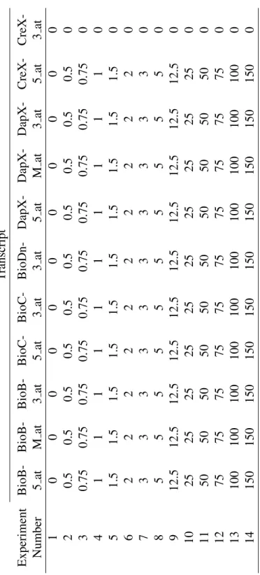
5.1 Probeset Groupings for the Affymetrix U95 Spike-In Study . . . 162
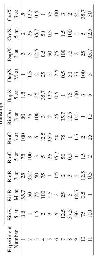
5.2 Concentration Data for the Affymetrix U95 Spike-In Study . . . 163
5.3 Probeset Groupings for the Affymetrix U133 Spike-In Study . . . 164
5.4 Concentration Data for the Affymetrix U133 Spike-In Study . . . 165
5.5 Concentration Data for the GeneLogic Tonsil Latin Square Dataset . . . 166
5.6 Concentration Data for the Choeet al.Golden Spike Dataset . . . 168
5.7 Clone and Pool Assignments for the Choe et al. Golden Spike Dataset Using Indirect Mappings . . . 186
5.8 Number of True Positives in Analysis of the GeneLogic Dilution Dataset . . . 187
5.9 Number of False Positives in Analysis of the GeneLogic Dilution Dataset . . . . 187
5.10 Number of True Negatives in Analysis of the GeneLogic Dilution Dataset . . . . 187
5.11 Number of False Negatives in Analysis of the GeneLogic Dilution Dataset . . . . 188
5.12 Statistical Significance for True Positives in the GeneLogic Dilution Analysis . . 188
5.13 Statistical Analysis of the Affymetrix U95 Latin Square Dataset . . . 189
5.14 Statistical Significance for the Affymetrix U95 Latin Square Analysis . . . 190
5.15 Statistical Analysis of the Affymetrix U133 Latin Square Dataset . . . 191
5.16 Statistical Significance for the Affymetrix U133 Latin Square Analysis . . . 191
C.1 Probesets Omitted from the Affymetrix U95 Latin Square and GeneLogic Dilu-tion Analysis . . . 370
C.2 Probesets Omitted from the Affymetrix U95 Latin Square and GeneLogic Dilu-tion Analysis . . . 371
C.3 Probesets Omitted from the Affymetrix U133 Latin Square Analysis . . . 372
1.1 Overview of cDNA Array Synthesis . . . 2
1.2 Overview of GeneChip Synthesis . . . 4
1.3 Photolithographic mask . . . 4
1.4 Probe Synthesis . . . 5
1.5 A Completed GeneChip . . . 5
1.6 Structure of a GeneChip . . . 6
2.1 Comparison of S-Score and RMA . . . 51
2.2 Comparison of S-Score and dChip . . . 52
2.3 Comparison of S-Score and MAS5 . . . 53
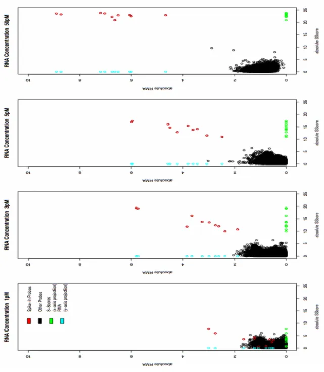
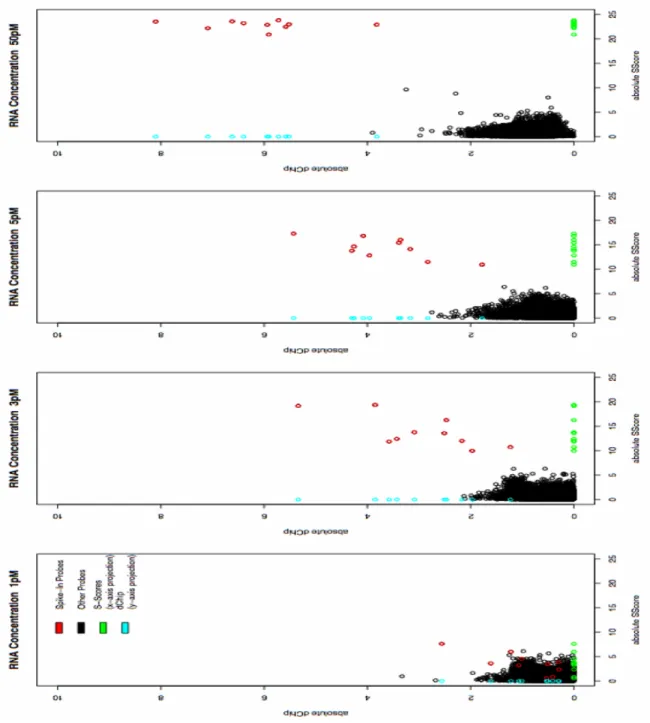
5.1 GeneLogic Dilution Quality . . . 179
5.2 GeneLogic AML Latin Square Quality . . . 180
5.3 GeneLogic Tonsil Latin Square Quality . . . 181
5.4 Affymetrix U95 Latin Square Quality . . . 183
5.5 Affymetrix U133 Latin Square Quality . . . 184
5.6 Choe Golden Spike Quality . . . 185
B.1 GeneLogic Dilution Quality, Experiments 1–4 . . . 353
B.1 GeneLogic Dilution Quality, Experiments 5–8 . . . 354
B.1 GeneLogic Dilution Quality, Experiments 9–12 . . . 355
B.1 GeneLogic Dilution Quality, Experiments 13–16 . . . 356
B.1 GeneLogic Dilution Quality, Experiments 17–20 . . . 357
B.1 GeneLogic Dilution Quality, Experiments 21–24 . . . 358
B.1 GeneLogic Dilution Quality, Experiments 25–26 . . . 359
B.2 Affymetrix U95 Latin Square Quality, Experiments 1–4 . . . 360
B.2 Affymetrix U95 Latin Square Quality, Experiments 5–8 . . . 361
B.2 Affymetrix U95 Latin Square Quality, Experiments 9–12 . . . 362
B.2 Affymetrix U95 Latin Square Quality, Experiments 13–16 . . . 363
B.2 Affymetrix U95 Latin Square Quality, Experiments 17–20 . . . 364
B.3 Affymetrix U133 Latin Square Quality, Experiments 1–4 . . . 365
B.3 Affymetrix U133 Latin Square Quality, Experiments 5–8 . . . 366
B.3 Affymetrix U133 Latin Square Quality, Experiments 9–12 . . . 367
B.3 Affymetrix U133 Latin Square Quality, Experiments 13–14 . . . 368
P probes or probe pairs . . . 10
S probesets . . . 10
M microarrays or arrays or chips . . . 10
C experimental condition or class . . . 10
D dye . . . 10
G gene . . . 10
L cell line . . . 10
N number of elements for a given level or variable . . . 10
AvgDi f f average difference . . . 12
M M mismatch probe intensity . . . 12
PM perfect match probe intensity . . . 12
IS set of rank-invariant probes . . . 16
i index or counter . . . 16
δ threshold for decision-making . . . 16
µ mean . . . 16
φ proportion of specific binding for MM probes . . . 16
ε random error term . . . 16
y intensity values for modeling (PMorPM−M M) . . . 16
Tbi(·) Tukey’s biweight function . . . 17
n number of observationsordegrees of freedom . . . 17
x observationorscalar input for function . . . 17
wbi(·) weight function for Tukey’s biweight . . . 18
u(·) uniform distance measure for Tukey’s biweight . . . 18
τ1 MAS5 tuning constant . . . 18
τ2 MAS5 tuning constant . . . 18
bZ MAS5 zone background . . . 18
(x,y) position coordinates . . . 18
wi(·) MAS5 weight function . . . 18
d(·,·) distance function . . . 18
τsm MAS5 smoothing constant . . . 18
SB MAS5 specific background . . . 19
I M idealized mismatch intensity . . . 19
τc MAS5 contrast tuning constant . . . 19
τs MAS5 scale tuning constant . . . 19
LV MAS5 log expression value . . . 19 vii
SF MAS5 scale factor . . . 20
EV MAS5 expression value . . . 20
tg target intensity value for scale normalization . . . 20
sg probe-specific signal . . . 20
bg nonspecific background signal . . . 20
σ2 variance . . . . 20
Y matrix of intensities . . . 21
n number of items in subsetordegrees of freedom . . . 24
A number of hypotheses accepted . . . 24
R number of hypotheses rejectedorcoefficient of variation . . . 24
α type I error rateornormalization constant . . . 24
FW ER family-wise error rate . . . 24
FDR false discovery rate . . . 25
HT number of true hypotheses . . . 25
HF number of false hypotheses . . . 25
H hypothesis . . . 25
T test statistic . . . 25
p p-value . . . 25
F(·) cumulative distribution function . . . 25
j index or counter . . . 25
q false discovery rate level of error . . . 25
(MG) array by gene interaction . . . 26
(CG) condition by gene interaction . . . 26
x design vector . . . 26
X design matrixormatrix input for function . . . 26
(C M) array by condition interaction . . . 27
ˆ ε residuals . . . 27
ψ random error term . . . 27
(MD) array by dye interaction . . . 28
(LC) cell line by condition interaction . . . 28
(LP) cell line by probe interaction . . . 28
(CP) condition by probe interaction . . . 28
kf rate constant for forward reaction . . . 32
kr rate constant for reverse reaction . . . 32
to total amount of probe for binding . . . 33
sc scale parameter for mmgMOS . . . 35
sh shape hyperparameter for mmgMOS . . . 35
ch scale hyperparameter for mmgMOS . . . 35
Ψ(·) digamma function . . . 36
Ψ0 (·) first derivative of the digamma function . . . 36
bv background variance (noise) . . . 40
γ fractional multiplicative error for intensity-dependent variance . . . 40
Z Z (normal or approximately normal) test statistic . . . 40
Φ(·) standard normal cumulative distribution function . . . 41
k number of parameters in full modelorrank of matrix . . . 56
a scalar hyperparameter for random variance model . . . 57
b scalar hyperparameter for random variance model . . . 57
r number of parameters in reduced model . . . 57
bβ maximum likelihood estimate of coefficients under null hypothesis . . . 58
b bβ maximum likelihood estimate of coefficients under alternative hypothesis . 58 Xω design matrix for reduced model . . . 58
c c S S sum of squares under null hypothesis . . . 58
c S S sum of squares under alternative hypothesis . . . 58
f S S sum of squares in random variance model . . . 58
z precision (inverse variance) parameter . . . 59
0 vector or matrix of zeros . . . 60
b σ2 estimated variance (mean squared error) . . . . 63
e σ2 estimated variance (mean squared error) in random variance model . . . . . 63
K number of free parameters . . . 63
u transformation variable for random variance model . . . 65
v transformation variable for random variance model . . . 65
b σ2 pooled pooled sample variance under null hypothesis . . . 67
t Student’s t test statistic . . . 67
e σ2 pooled pooled sample variance in random variance model . . . 67
et modified t test statistic in random variance model . . . 67
F Snedecor’s F test statistic . . . 67
e F modified F test statistic in random variance model . . . 67
bv SScore mean background . . . 72
y SScore mean intensity . . . 73
lm difference in log intensity between conditions . . . 76
y average log intensity of conditions . . . 76
Q quantiles . . . 76 O groups . . . 76 ξ median of observations . . . 76 σ variance of observations . . . 76 ϕ(·) permutation function . . . 80 cf cofactor of a matrix . . . 80 ζ scalar constant . . . 81 λ eigenvalue . . . 81 e eigenvector . . . 81
L diagonal matrix of eigenvalues . . . 81
E matrix of eigenvectors . . . 81
Ip identity matrix . . . 81
X1/2 matrix square root . . . 82
X∗ lower triangular decomposition . . . . 82
v vector . . . 85
Lp elimination matrix . . . 87
Dp duplication matrix . . . 88
Np symmetrizer matrix . . . 88
h limit constant for derivative . . . 97
r(·) scalar remainder function . . . 97
E set of matrices on which a function is defined . . . 100
B(·,·) ball (neighborhood) about a matrix . . . 100
rd radius . . . 100
U matrix within the neighborhood of a specified matrix . . . 100
A (first) derivative matrix . . . 100
Rc matrix remainder function . . . 100
G(·) matrix-valued function . . . 101
H(·) matrix-valued function . . . 101
C constant matrix . . . 101
η eigenvalues . . . 113
Q transformation matrix for singular matrices . . . 115
M random matrix . . . 117
Γp(·) multivariate gamma function . . . 117
Ξ location parameter matrix . . . 125
Ω scale parameter matrix . . . 125
Λ Wilk’s lambda statistic . . . 129
B matrix hyperparameter for random variance model . . . 130
Z precision (inverse covariance) matrix in random variance model . . . 132
O intermediate result of matrix calculations . . . 136
bΣ sums of squares and crossproducts under alternative hypothesis . . . 138
b bΣ sums of squares and crossproducts under null hypothesis . . . 139
f SS sums of squares and crossproducts in random variance model . . . 139
U transformed matrix in random variance model . . . 141
AI Adaptive Interval
AML acute myeloid leukemia
ANOVA analysis of variance
AUC area under the curve
CDF cumulative distribution function
cDNA complementary deoxyribonucleic acid
CLT Central Limit Theorem
cRNA complementary ribonucleic acid
DNA deoxyribonucleic acid
FDR false discovery rate
FWER family-wise error rate
GCOS GeneChip Operating Software
GLM general linear model
ISH in situhybridization
IVT in vitrotranscription
LPE local pooled error
MAD median absolute deviation
MANOVA multivariate analysis of variance
MAQC MicroArray Quality Control
MAS4 Microarray Suite version 4.0
MAS5 Microarray Suite version 5.0
MBEI model-based expression index
MLE maximum likelihood estimate
MM mismatch
mmgMOS multichip modified gamma model of oligonucleotide signal
mRNA messenger ribonucleic acid
PCR polymerase chain reaction
PRD proportional rank difference
PM perfect match
PPV positive predictive value
RIR rank invariant resampling
RMA robust multi-chip average
RNA ribonucleic acid
ROC receiver operating characteristic
RVM Random Variance Model
SAM Significance Analysis of Microarrays
SDT Statistical (or Standard) Difference Threshold
SF Scale Factor
PROBE LEVEL ANALYSIS OF AFFYMETRIX MICROARRAY DATA By Richard Ellis Kennedy, Ph.D.
A dissertation submitted in partial fulfillment of the requirements for the degree of Doctor of Philosophy at Virginia Commonwealth University.
Virginia Commonwealth University, 2008
Major Director: Kellie J. Archer, Ph.D. Assistant Professor
Department of Biostatistics
The analysis of Affymetrix GeneChipR data is a complex, multistep process. Most often,
meth-ods condense the multiple probe level intensities into single probeset level measures (such as ro-bust multi-chip average (RMA), dChip and Microarray Suite version 5.0 (MAS5)), which are then followed by application of statistical tests to determine which genes are differentially expressed. An alternative approach is a probe-level analysis, which tests for differential expression directly using the probe-level data. Probe-level models offer the potential advantage of more accurately capturing sources of variation in microarray experiments. However, this has not been thoroughly investigated, since current research efforts have largely focused on the development of improved expression summary methods. This research project will review current approaches to analysis of probe-level data and discuss extensions of two examples, the S-Score and the Random Variance
Model (RVM). The S-Score is a probe-level algorithm based on an error model in which the detected signal is proportional to the probe pair signal for highly expressed genes, but approaches a background level (rather than 0) for genes with low levels of expression. Initial results with the S-Score have been promising, but the method has been limited to two-chip comparisons. This project presents extensions to the S-Score that permit comparisons of multiple chips and “bor-rowing” of information across probes to increase statistical power. The RVM is a probeset-level algorithm that models the variance of the probeset intensities as a random sample from a common distribution to “borrow” information across genes. This project presents extensions to the RVM for probe-level data, using multivariate statistical theory to model the covariance among probes in a probeset. Both of these methods show the advantages of probe-level, rather than probeset-level, analysis in detecting differential gene expression for Affymetrix GeneChip data. Future research will focus on refining the probe-level models of both the S-Score and RVM algorithms to increase the sensitivity and specificity of microarray experiments.
Introduction
1.1
Overview of Microarray Technology
The development of microarray chips has had a profound impact on the design of gene expression studies (Shiet al., 2006). Microarrays allow the large-scale analysis of expression changes across thousands of genes at once, in contrast to previous small-scale methods that were restricted to examining the expression of only a few genes at a time. Advances in technology have led to chips that are essentially capable of analyzing expression values across the entire genome simultane-ously (Dalma-Weiszhauszet al., 2006).
1.1.1
cDNA Array Design
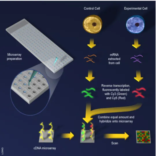
Microarrays are broadly divided into two categories, custom spotted or complementary deoxyri-bonucleic acid (cDNA) arrays and oligonucleotide arrays (Nguyenet al., 2002). The former are designed by synthesizing complementary probes to messenger ribonucleic acid (mRNA) obtained from biological samples using reverse transcription (Schenaet al., 1995), as shown in Figure 1.1. For custom spotted arrays, segments from genes of interest are amplified using the polymerase chain reaction (PCR) to attain sufficient quantities of deoxyribonucleic acid (DNA). These DNA fragments are then placed on glass microscope slides or a similar substrate in a high-density grid pattern using a robotic pin arrayer or inkjet printer. The instrumentation is relatively inexpensive compared to that needed for oligonucleotide chips, so cDNA arrays may be produced by local
Figure 1.1: Overview of cDNA Array synthesis. DNA fragments are created using PCR and bound to glass microscope slides. These DNA fragments hybridize to complementary targets from samples. Image courtesy of Science Creative Quarterly (http://scq.ubc.ca), Jiang Long, artist.
laboratories or obtained commercially (Hardiman, 2004; Hager, 2006). Next, mRNA from two samples, one representing the experimental condition and one representing the control condition, are extracted and reverse transcribed into cDNA. The cDNA is labeled with fluorescent dye; by convention, Cyanine 5 (Cy5, a red fluorescent dye) is used for the experimental condition and Cyanine 3 (Cy3, a green fluorescent dye) is used for the control condition. The two samples are then mixed in equal proportion and hybridized to the array. The array is then imaged using a fluorescent scanner, with separate images collected for the red and green channels. The relative signal intensity between the two channels is assumed to be proportional to the relative abundance of the gene sequence of interest in the two samples (Dugganet al., 1999).
1.1.2
Oligonucleotide Array Design
Oligonucleotide microarrays are designed by chemically synthesizing small nucleotide fragments with a predefined sequence (Lipshutzet al., 1999). The Affymetrix GeneChipR oligonucleotide
microarray is one of the most widely used and best standardized platforms for large-scale analysis of gene expression data (Wuet al., 2004), although other platforms are available (Fanet al., 2006; Wolber et al., 2006; Shi et al., 2006; Singh-Gasson et al., 1999). An overview of GeneChip manufacture can be found in Dalma-Weiszhauszet al. (2006) and is shown in Figure 1.2. The basic unit for GeneChip design is aprobe, a single 25-mer intended to hybridize with a specific transcript of a specific gene, which is called the target sequence. The target sequence reported by Affymetrix represents a “consensus” sequence for a particular gene, using information derived from public repositories and other sources (Alberts et al., 2007). Target sequences are intended to be unique for a particular gene; however, it is recognized that this does not hold for a number of targets (Stalteri and Harrison, 2007; Gautieret al., 2004). A complete list of target sequences for current and past varieties of GeneChips is available at the Affymetrix website (http://www. affymetrix.com).
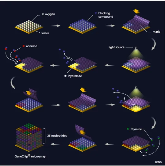
GeneChips containing complementary probes to the target sequences are constructed using photolithography (Dalma-Weiszhauszet al., 2006). For this process, quartz wafers are modified with silane material to allow covalent attachment of nucleosides to the chip. A photolithographic mask containing windows to permit the transmission of ultraviolet light is then aligned with the wafer. The windows on the mask are spatially distributed over the mask to correspond to the se-quence for each probe. The application of near-ultraviolet light activates the exposed (windowed) areas of the wafer for nucleoside bonding, while unexposed areas remain protected (Figure 1.3). The wafer is then flushed with a nucleoside-containing solution, and the nucleoside attaches at the activated sites. This process, which lengthens all activated probes by one nucleotide, alternates through the four nucleosides (A, C, G, and T) repeatedly to create 25-mers with the appropriate sequence in the appropriate spatial position on the wafer (Figure 1.4). Wafers are then diced and packaged individually into cartridges (Figure 1.5).
Figure 1.2: Overview of GeneChip synthesis. Nucleosides are progressively added to a silanized chip by photolithography to create a set of 25-mers matching specific sequences. Image courtesy of Science Creative Quarterly (http://scq.ubc.ca), Jiang Long, artist.
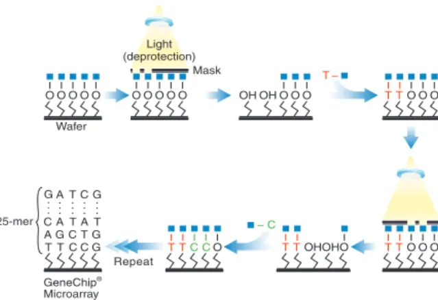
Figure 1.3: Activation of selected areas of a GeneChip using a photolithographic mask. Only probes in activated areas (shown in yellow) will be extended by the next application of nucleoside solution. Image courtesy of Affymetrix.
Figure 1.4: Synthesis of probes occurs in cycles, in which activated cells are lengthened by one nucleotide. Image courtesy of Affymetrix.
Figure 1.6: Structure of a GeneChip. Image courtesy of Affymetrix.
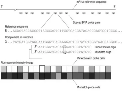
Probes are synthesized in sets of two called probe pairs (Figure 1.6). Each pair consists of a perfect match (PM) and a mismatch (MM) probe. The PM probe matches the target sequence exactly and is intended to measure specific signal for a particular gene. The MM probe has an inversion at the middle (13th) base and is intended to measure nonspecific binding of the
probe. Unfortunately, the PM probe may bind nonspecifically to other similar sequences (Wu and Irizarry, 2005), and the MM probe may have a specific binding component to the target sequence (Wuet al., 2004); both effects have significant implications for the analysis of microarray data. A probe setconsists of a group of 11 to 20 probe pairs, which are related by the fact that each pair interrogates a region on the same gene (Figure 1.6). This level of redundancy in the pairs of a probeset is intended to produce more accurate estimates of gene expression. There may be one or more probesets interrogating the same gene. For current chips, the majority of genes have only a single associated probeset. Finally, a GeneChip consists of thousands of probesets that interrogate multiple genes (Figure 1.6).
With the commercial Affymetrix GeneChip, one array is used for each sample in the exper-iment. The hybridization material for the arrays typically consists of mRNA isolated from the study samples, although DNA fragments have also been used. When mRNA is the starting mate-rial, a single strand of cDNA is produced through reverse transcription, followed by synthesis of
a second strand to produce double-stranded cDNA. Such steps are not necessary with DNA as a starting material. Next, anin vitrotranscription (IVT) process is performed according to standard molecular biology procedures (Van Gelder et al., 1990). This amplifies the target ribonucleic acid (RNA) for subsequent hybridizations. The use of biotinylated nucleosides in the IVT reac-tion allows subsequent detecreac-tion of the target. The target RNA is then hybridized to the GeneChip and stained with a streptavidin-phycoerythrin conjugate using standard protocols available from Affymetrix (Affymetrix, 2002a). Following hybridization, the array is imaged using a fluorescent scanner. The fluorescent signal intensity is assumed to be proportional to the abundance of the target for each probe (Chudinet al., 2002).
1.1.3
Comparison of cDNA and Oligonucleotide Array Technologies
Oligonucleotide and cDNA technologies represent two different approaches to the quantification of gene expression using microarrays. Recent studies have shown that the two are generally com-parable in achieving this goal, and choice between platforms should be made based on other fac-tors (Pattersonet al., 2006). Oligonucleotide chips require that the entire sequence of the target be known, while cDNA chips only require knowledge of the primer sequences for PCR (Hardiman, 2004). This can offer significant advantages in the study of less well characterized genes. The cDNA arrays are more easily customized (Hager, 2006), although made-to-order oligonucleotide chips are available (Dalma-Weiszhauszet al., 2006). The cost per array is substantially lower for cDNA arrays, which may be produced using equipment available in most molecular biology lab-oratories (Hager, 2006). However, cDNA arrays may require dye swap experiments to separate dye effects from experimental effects, which may increase the number of arrays and offset any cost savings (Dobbinet al., 2003). The quality of cDNA arrays that are not mass produced may be inferior to that of commercial oligonucleotide chips (Hardiman, 2004). Finally, the choice be-tween cDNA and oligonucleotide arrays can have a significant influence on experimental design and analysis, as described in the next section.
1.2
Experimental Design
1.2.1
Introduction
Study design plays a critical role in obtaining meaningful results from microarray experiments (Reimers, 2005). It also has a significant influence on the selection and application of statistical tests that are used in the analysis. Traditional statistical topics such as power, randomization, and validation of model assumptions apply to microarray studies in a manner similar to biomedical studies, although these areas may receive insufficient attention in the planning of microarray experiments (Bolstad et al., 2004). However, microarray experiments also have unique features not found in other types of studies, which are reviewed in this section. Detailed reviews of the topic for both cDNA and oligonucleotide arrays may be found in Bolstadet al.(2004), Churchill (2002), Kerr and Churchill (2001), and Simonet al.(2002).
One issue common to both cDNA and oligonucleotide arrays is replication (Allison et al., 2006). Replication is essential for differentiating systematic variation due to treatment or phe-notypic effects from chance variation (Lee, 2001). For microarray experiments, two types of replicates are possible, technical and biological(Yang and Speed, 2002). Technical replication occurs when RNA from the same extraction is hybridized to multiple chips. Biological replication occurs when RNA from different extractions of the same sample is hybridized to multiple chips, or when RNA from different samples within the same condition is hybridized to multiple chips. The variability associated with biological replicates is generally greater than that with technical replicates, as the variability between individuals (or extractions) is generally greater than variabil-ity in the hybridization and processing of chips. Technical replicates reduce variabilvariabil-ity, but only provide information about the variability within a particular extraction. In contrast, biological replicates provide information about the variability between individuals (or extractions), mak-ing the experimental results more generalizable. A combination of both technical and biological replicates is ideal, but biological replicates are preferred over technical replicates for both cDNA and microarray studies. Additional aspects of experimental design unique to each platform are
reviewed in the following sections.
1.2.2
Experimental Design of cDNA Microarray Studies
With the hybridization of two samples on a single array, cDNA experiments are inherently com-parative (Yang and Speed, 2002). The results of a cDNA study measure the relative abundance of the target sequence in the experimental sample to that in the control sample. Since a control sample is hybridized to each chip, the arrangement of controls deserves special consideration (Churchill, 2002; Yang and Speed, 2002). For designs such as the comparison of gene expression pre- and post-treatment across several samples, the choice of control can be straightforward. How-ever, with other types of experiments, such as the comparison of several experimental samples to a single control sample, the choice is less clear. More complicated designs, such as the common reference design and the loop design, frequently appear in cDNA studies. The latter designs are amenable to analysis with traditional statistical methods such as general linear models (GLMs), but introduce an added layer of complexity in the analysis.
Another consideration in the design of cDNA experiments is the effect of cohybridizing two samples to the same array simultaneously. This approach does have advantages, for it removes extraneous components of between-chip variability (such as differences in chip manufacturing or handling) when comparing the two samples on the chip (Dugganet al., 1999). However, without appropriate care, it can also introduce unintended sources of confounding. Systematic differences between the red and green dyes can occur in the incorporation stage and in the scanning stage (Dobbin et al., 2003). If not properly addressed, these dye biases can be mistaken for treat-ment effects. Dye-swap designs, in which the dyes for the experimental and control samples are swapped for different hybridizations, can be useful in overcoming this bias but at the expense of additional cost and complexity of analysis.
1.2.3
Experimental Design of Oligonucleotide Microarray Studies
In contrast to cDNA arrays, only one sample is hybridized to each chip for oligonucleotide arrays. This can greatly simplify experimental design, making the process very similar to experimental design for biomedical studies, which has been extensively investigated (Bolstad et al., 2004). Thus, variations of the GLM are the most frequently used approach (Jafari and Azuaje, 2006). However, the use of one sample per chip may potentially confound differences in chip manufac-turing and processing with treatment differences (Gebicke-Haerter, 2005). Replication can help prevent this bias, as can appropriate use of randomization in the processing phase, although the latter may not be adequately considered in many microarray experiments. Preprocessing proce-dures such as normalization are intended to reduce this bias once it occurs, although this only achieves a partial correction (Bolstadet al., 2004).
1.2.4
Notational Conventions
Notation used in the experimental design of microarray studies varies considerably by author. In all subsequent sections, probes (or probe pairs) will be designated using the variable P and the subscript p, probesets with the variableS and subscript s, arrays or chips with the variable M
and subscript m, and experimental conditions or classes with the variableC and subscript c. In cDNA array models, dye will be designated using the variableDand subscriptdand gene, which roughly corresponds to the probeset variable for oligonucleotide arrays, will be designated with the variableG and subscriptg. For those experiments having both cell lines and treatments, the former will be denoted with the variable Land subscript `, and the latter with the subscript for condition. The variable N with the appropriate subscript will be used to denote the number of elements at that level. For example, Np will denote the number of probes within a probe set,
which may vary from probeset to probeset. Scalar quantities will be denoted with italicized Ro-man or Greek letters, which may be upper- or lowercase, and the upper- and lowercase variables are distinct. Vector quantities will be denoted with bold lowercase and matrix quantities with bold uppercase Roman or Greek letters. This may lead to slight notational differences from the
original, cited articles, although the meaning will remain the same. Abbreviations for the clas-sifications of differential gene expression produced by software, such as P for present and A for absent, are not intended to represent variables and will not be italicized.
1.3
Image Analysis
Following hybridization, both cDNA and oligonucleotide arrays are scanned using a fluorescent scanner, producing an image of the chip with areas of higher intensity corresponding to areas of greater target concentration. This image is stored as a graphics file, typically using the tagged image file format (TIFF) structure. The process of image analysis converts this graphics file into a series of numerical values, one for each probe, which represents the signal intensity for that probe. This is a complex process involving three steps: gridding, which assigns coordinates to the pixels on the chip; segmentation, in which each pixel in the image grid is classified as background or signal, andintensity extractionorquantification, in which a single overall estimate for the signal intensity for the probe is computed from the set of pixels representing signal for that probe (Yang
et al., 2001). Image analysis produces a file of signal intensities, whose exact format varies by platform, which are suitable for expression analyses as detailed in the following sections. Algorithm development for image analysis is an active area of research; an overview of the topic for cDNA arrays is given by Jain et al. (2002) and Yang et al. (2001) and for oligonucleotide arrays by Schadtet al.(2001).
For Affymetrix GeneChips, image analysis produces a CEL file, which contains information about the experiment and the probe intensities. The first component of the CEL file is a header section, which details the physical characteristics of the chip and the parameters for the image analysis. This is followed by an intensity section, which gives the physicalxandycoordinates of the probe on the chip, the number of pixels assigned to the probe, and the mean and standard devi-ation for the probe based on the pixel intensities. Next is a section giving the coordinates of probes that are outliers. The final two sections identify masked probes that are removed from analysis by the user and modified probes with intensities that are assigned by the user; these are listed in the
final two sections. Using this format, the CEL file provides all of the data necessary for analysis of individual microarrays. Further details of the CEL file format are available from the Affymetrix website at http://www.affymetrix.com/Auth/support/developer/fusion/file formats.zip.
1.4
Early Methods for Computing GeneChip Expression
One of the first widely used methods for analysis of GeneChip data was the Affymetrix Microar-ray Suite version 4.0 (MAS4) algorithm, also called the Empirical Expression algorithm (Aff y-metrix, 2004). As the CEL file format was originally proprietary, MAS4 was thede facto stan-dard for expression analysis of Affymetrix data in early studies. It also introduced the concepts of background correction and summarization for GeneChip data, which have been incorporated in the preprocessing step of later algorithms for Affymetrix expression analysis.
The full details of the MAS4 algorithm have not been published, but a limited description is provided in the Affymetrix MAS4 User’s Guide and the GeneChip Operating Software (GCOS) manual (Affymetrix, 2004). For single array analyses (or for each chip in a multi-chip compari-son), the MAS4 algorithm generates three different metrics comparing the PM and MM intensities of each probe pair in a probe set. These metrics are then weighted and entered into a decision matrix to determine theabsolute call, which represents the overall status of the probeset on the chip. The absolute call is simply a classification of present (P), marginally present (M), or absent (A) for each probeset. In addition, the MAS4 algorithm calculates the AvgDi f f value for each probeset, which is a relative measure of the level of expression for the probeset. TheAvgDi f f for thesth probeset is defined as
AvgDi f fs= 1 Np Np X p=1 PMsp−M Msp (1.1)
whereNpis the number of probe pairs in probesetsafter trimming values with extremely strong
or extremely weak intensity values. Background correction is performed by subtracting theM M
obtain an estimate of specific binding. The multiple probe-level values are then summarized into a single expression index for the probeset using the arithmetic mean.
Comparisons between arrays in the MAS4 algorithm are made by comparing each experimen-tal array in turn to a user-selected baseline array. The algorithm generates five different metrics for each comparison. These metrics are then weighted and entered into a decision matrix to de-termine thedifference call, which represents the status of the probeset on the experimental array relative to the baseline array. The difference call classifies the changes in expression for each probeset as increased (I), mildly increased (MI), no change (NC), mildly decreased (MD), or de-creased (D). No original validation studies of the MAS4 algorithm were published, although it has been used in peer-reviewed publications.
1.5
Current Methods for Computing GeneChip Expression
1.5.1
Introduction
The development of MAS4 represents a significant step forward in the analysis of microarray data, as it provided a standard index of expression that corresponds to concentration in many circumstances (Hubbellet al., 2002). However, investigators quickly realized some of the limita-tions of the MAS4 algorithm. The estimates are sensitive to outliers (Hubbellet al., 2002). Given the large number of probes on a GeneChip, the presence of outliers is quite likely and can dramat-ically influence results. The use of the raw M M probe values to estimate nonspecific binding is also problematic, as theM M value exceeds thePMvalue for about a third of the probes (Irizarry
et al., 2003). This corresponds to a negative estimate of the target concentration, a physical im-possibility. Furthermore, the negative estimates preclude the use of many transformations, such as the logarithmic, that are commonly used in statistics.
With the release of the Affymetrix file formats into the public domain (available at http:// www.affymetrix.com/Auth/support/developer/fusion/file formats.zip), many researchers began to develop their own analytical algorithms to correct the deficiencies of MAS4. In the following
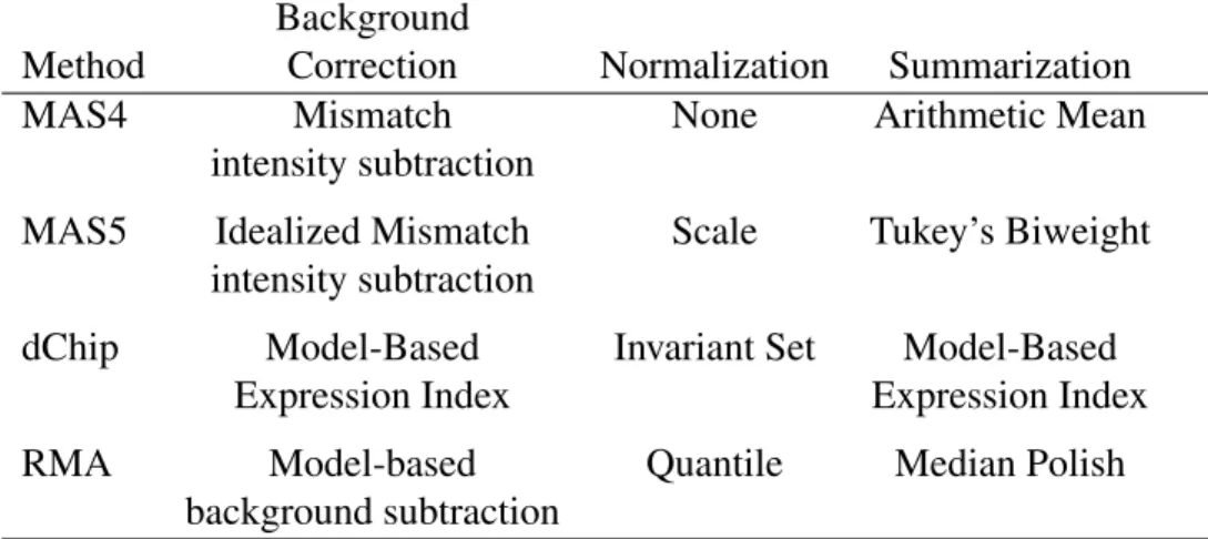
Background
Method Correction Normalization Summarization MAS4 Mismatch None Arithmetic Mean
intensity subtraction
MAS5 Idealized Mismatch Scale Tukey’s Biweight intensity subtraction
dChip Model-Based Invariant Set Model-Based Expression Index Expression Index RMA Model-based Quantile Median Polish
background subtraction
Table 1.1: Overview of Probeset Summary Methods for Affymetrix Data.
sections, the shared features of these algorithms will be presented, followed by specific details of some of the more commonly used ones. These examples will illustrate the variety of approaches currently used in microarray data analysis and serve as a reference for methods used in later comparative studies. An overview of these algorithms is presented in Table 1.1.
1.5.2
Pre-processing
Most algorithms for Affymetrix data that are in current use perform pre-processing of the mi-croarray data. Pre-processing is intended to correct potential problems when obtaining intensity values for the probesets on a GeneChip, thus preparing the data from image analysis algorithms for statistical analysis to detect differential gene expression (Bolstadet al., 2005). Pre-processing consists of three steps: background correction, normalization, and summarization. Background correction removes the signal resulting from nonspecific binding of target to probe. Specific bind-ing occurs due to complementary base-pairbind-ing between the two sequences, and the goal of gene expression studies is to measure specific binding precisely (Wu and Irizarry, 2005). Nonspecific binding occurs due to other factors, spuriously increasing the detected signal. The M M probe in a probe pair is intended to measure this nonspecific binding, so that the PM− M M difference would be specific binding (Wu and Irizarry, 2005). However, the relationship has proven to be more complex, as the M M probe measures some specific as well as nonspecific binding (Wu
et al., 2004). Because of this, some investigators have chosen only to use PM probes for esti-mation of background, while others estimate the background with models utilizing bothPM and
M M values (Li and Wong, 2001).
Normalization adjusts the probe intensities to make measurements between different chips comparable (Bolstadet al., 2003). Variations in the intensity measurements between samples are expected to occur due to differential gene expression. However, another level of variation occurs for reasons other than biological differences, which Bolstadet al.callobscuring variation; these sources of variation can include technical differences in sample preparation, hybridization, and scanning (Zakharkinet al., 2005). This additional variation leads to differences in the distribution of the probe intensities among chips, making direct comparisons difficult. Normalization manip-ulates the probe intensity distributions in an attempt to minimize obscuring variation, so that valid statistical comparisons of the remaining biological variation can be performed.
Summarization combines the information from the many probes targeting a gene into a single number representing the expression level for that gene. From a statistical standpoint, this is a data reduction, which can be useful for reducing the time and complexity of subsequent calculations. The results of summarization also correspond to the biological question being posed, as expres-sion differences between genes, rather than expression differences between probes, are usually of interest.
1.5.3
dChip
One of the first widely-used alternatives to MAS4 was the algorithm used in the dChip software (Li and Wong, 2001; Li and Hung Wong, 2001). For normalization, dChip uses the invariant set method, which attempts to base normalization only on those probes that are not differentially expressed between chips (Li and Hung Wong, 2001). Such probes would be expected to have similar (but not necessarily identical) intensity-based ranks between two chips, with one chip identified as the baseline and the other as the chip to be normalized. The procedure to identify these probes, called the invariant set, is detailed in Algorithm 1.1.
Algorithm 1.1Identification of Invariant Set
1: Initialize the invariant set at iteration zeroIS(0)to the set of all PM probes for the two chips.
2: For iterationi, calculate the proportional rank difference (PRD), defined as the rank difference between the two chips divided by the number of probes per chip, for each of the PM probes in the datasetIS(i).
3: If the PRD for a probe is less than the thresholdδ, defined as δ = 0.003 for low intensity probes andδ <0.007 for high intensity probes, then retain the probe for the datasetIS(i+1)of the next iteration. (The different thresholds allow for the sparsity of probes at the upper tail of the intensity distribution.)
4: Repeat steps 2 and 3 until the invariant set does not change between iterations.
5: Fit a piecewise linear running median line using the invariant set and perform normalization by projecting the intensities of the chip to be normalized onto the line.
For background correction and summarization, dChip calculates a model-based expression index (MBEI). This uses a statistical model for the probe intensities that assumes the intensity is directly proportional to the expression index (or microarray effect) M for array m, but that the proportionality constant may differ by probe. Furthermore, the increase in PMintensity will always be greater than the increase inM M intensity. The model is
M Mmp =µp+Mmφp+εmp (1.2) PMmp= µp+Mmφp+MmPp+εmp (1.3)
where µis the baseline intensity for the pth probe due to nonspecific binding, φis the propor-tionality constant for the M M probe due to specific binding,Pis the proportionality constant for the PM probe due to specific binding, and the error term ε∼ N0, σ2. For identifiability, the
constraintPNp
p=1Pp = Npis also imposed.
In the original model (Li and Wong, 2001), thePM−M M differences are used as the estimate of the specific binding for the probe
ymp= PMmp− M Mmp= MmPp+εmp (1.4)
Estimates of the parameters are found using Equation (1.4). An iterative least squares fitting is performed for M and for P, with one parameter being fit while holding the other parameter
constant. The interpretation of theM Msignal intensity can be problematic, so Li and Hung Wong (2001) later constructed a PM-only model
PMmp= µp+MmPp+εmp
This model is fit using iterative least squares, similar to thePM−M Mmodel. Unfortunately, the use of the dChip algorithm requires a rather large number of arrays to obtain accurate estimates; Li and Wong recommend 10 or more for most experiments. The software is available at the dChip website (http://www.dchip.org). The algorithm is also implemented in thefit.li.wongandexpresso
functions in the R packageaffy. However, since the dChip software is not open source, the latter two functions do not exactly reproduce the results of the former.
1.5.4
MAS5
The MAS5 algorithm was developed by Affymetrix as a successor to MAS4 (Liu et al., 2002; Hubbellet al., 2002). MAS5 made significant changes to the background correction, normaliza-tion, and summarization procedures to overcome deficiencies noted in MAS4.
MAS5 makes extensive use of the one-step Tukey’s biweight procedure, which is a robust measure of central tendency somewhat similar to a weighted mean (Hoaglin et al., 2000). It is based on a uniform distance measure is calculated for each observation, with standardization using the median and median absolute deviation (MAD). The biweight value then calculated as a weighted average of each of the observations. The weight function is chosen to give a weight that decreases with distance for observations within a certain distance from the median, and a zero weight for observations outside of this distance from the median. Tukey’s biweightTbi(·) for the nobservations x1,x2, . . . ,xnis formally defined as
Tbi(x1,x2, . . . ,xn)=
Pn
i=1wbi(ui)xi
Pn
wherewbi(·) is the weight function wbi(xi)= 1−[ui(xi)]2 2 , |ui(xi)| ≤1 0, |ui(xi)|>1
andu(·) is the uniform distance measure
ui(xi)=
xi−median (x1, . . . ,xn)
τ1·MAD (x1, . . . ,xn)+τ2
Both τ1 and τ2 are user-defined tuning constants specified in the MAS5 software. Tukey’s
bi-weight can be computed by iteratively rebi-weighting the estimates until convergence occurs, but the one-step estimation used by MAS5 will generally produce acceptable results (Hoaglinet al., 2000).
For background correction, MAS5 uses a multistep process to ensure that negative intensity estimates do not occur. Each chip is divided into an Nz × Nz set of rectangular regions, called zones. The zone background bZ is the average of the lowest 2% of probe intensities for each zone. The backgroundbgfor a probe at position (x,y) on the chip is calculated as a weighted sum of the zone background values, which smoothes the transition between zones:
bg= 1 PNz2 i=1wi(x,y) Nz2 X i=1 wi(x,y)bZi (1.5)
wherewi(·) is the weight function
wi(x,y)=
1
d2
i (x,y)+τsm
(1.6)
andd(·,·) is a distance function, the form of which is not specified by Affymetrix. Here the (x,y) coordinates of a zone are defined to be the center of the zone, and τsm is a user-defined tuning
constant for adjusting the degree of smoothing. The background value for each probe subtracted from the PM and MM intensities for that probe; any negative values are replaced by a user-defined
fraction of the noise for that probe. Next, a probeset-level specific backgroundSBfor probeset s
is calculated as
SBs =Tbi
log2PMs1−log2M Ms1, . . . ,log2PMs,Np −log2M Ms,Np
Background correction concludes with the calculation of the idealized mismatchI M. ThePM−
I M value is intended to measure specific binding, but unlike the PM− M M value is guaranteed never to be negative. The formula for theI Mvalue is
I Msp= M Msp, M Msp< PMsp PMsp 2SBs , M Msp≥ PMspandSBs > τc PMsp 2 τc 1+ τc−SBs τs , M Msp≥ PMspandSBs ≤τc
whereτcandτsare user-defined tuning constants (contrast and scale, respectively) for weighting
the relative importance of probe- and probeset-level information in the calculation. Using this formula, if the MM value is already lower than thePMvalue, thenM M is a reasonable estimate of nonspecific binding and is used for theI M value. Otherwise, the I M value is calculated as a fraction of thePMvalue. If specific backgroundSBis “large” (as defined using theτcparameter),
then the intensities from the probeset are generally reliable, and theI Mvalue that is constructed is not specific to the individual probe but does use information restricted to the associated probeset. If SB is “small”, the intensities from the probeset are less reliable, and the I M value that is constructed is only weakly related to the probe- and probeset-specific information.
Summarization in MAS5 creates a single expression log valueLV for each probeset by taking the Tukey’s biweight of the log difference between thePMandI Mvalues:
LVs= Tbi log2(PMs1−I Ms1), . . . ,log2 PMs,Np −I Ms,Np
Normalization in MAS5 is performed by conducting a scale normalization, which adjusts all chips to have the same mean intensity. This is done by calculating a scale factor SF to adjust the 2% trimmed mean to a user-defined target intensity value, then multiplying the unadjusted expression values by the scale factor to obtain the final expression valuesEV.
SF = tg
TrimMean (2LVs,0.02,0.98)
EVs= SF·2LVs
MAS5 is implemented in the GCOS software available from Affymetrix. It is also implemented in theexpressoandmas5functions in the R packageaffy, available from the Bioconductor project (http://www.bioconductor.org). However, the latter two functions do not exactly reproduce the results of the Affymetrix software, as they were developed prior to the release of the GCOS software as open source (see http://www.affymetrix.com/support/developer/stat sdk/index.affx).
1.5.5
RMA
The robust multi-chip average, or RMA (Irizarry et al., 2003), is one of the most widely used expression measures and a standard choice for comparing the performance of new algorithms. RMA utilizes only the PM value in calculations. For background correction, the observed in-tensities are modeled as a combination of probe-specific signal sg and nonspecific background
bg:
PMmsp = sgmsp+bgmsp
where sg has an exponential distribution, bg ∼ N0, σ2, and sg and bg are independent of each other. Background adjustment is accomplished by estimating the probe-specific intensities
Esgmsp|PMmsp
For normalization, RMA uses the quantile normalization method (Bolstadet al., 2003). It is an aggressive form of normalization that forces each chip to have the same distribution of inten-sities. This is accomplished by transforming all chips to a common distribution, standardizing, and then back-transforming each chip individually, as shown in Algorithm 1.2. The elements of
Algorithm 1.2Quantile Normalization
1: Arrange themmicroarrays, each withpprobesets, into am× pmatrixY
2: Sort each column ofYindividually to giveYsort
3: Compute the row means ofYsort
4: Assign the row mean to each element of the row to giveYad j
5: Rearrange each column ofYad jinto the original unsorted order inY to giveYnorm
Ynorm, denoted byy, represent the quantile-normalized intensities that are used in subsequent
com-putations. Because quantile normalization forces the same distribution across chips, the authors recommend that normalization only be performed on similar chips.
For computing expression summary values, RMA fits the background-adjusted, quantile-normalized, and log2-transformedPMintensitiesyto the additive model
ymsp= µs+Psp+Mms+εmsp
whereµdenotes the overall mean for the probeset,P represents the probe affinity effect, and M
represents the array effect, and the error termε∼ N0, σ2. The estimate ˆµ+Mˆ
msis the probeset
expression summary for probesetson arraym. This model is fit using an iterative median polish procedure, which is a robust method of fitting an additive model that is in some ways analogous to analysis of variance (ANOVA) (Hoaglin et al., 2000, chapter 6). This procedure iteratively subtracts the median across each factor (median polish) to obtain successive approximations for the factor effects, as shown in Algorithm 1.3. Iterations may be carried out until convergence, which occurs when the residuals after the median polish are zero across all factors, but a small number of iterations are generally sufficient to give good estimates of the factor effects. The RMA algorithm is available in thermaandexpressofunctions in the R package affy, as well as the stand-alone RMAExpress software (http://rmaexpress.bmbolstad.com/).
Algorithm 1.3Median Polish
1: Initialize the residuals to the intensity data.
ε(0)
msp ←ymsp
2: Initialize the row (probe), column (array), and overall (mean) effects to 0.
µ(0)
s ←0
P(0)sp ←0 Mms(0) ←0
3: Row polish by subtracting row (probe) medians
∆P(spi) ← median ε(i−1) 1sp , . . . , ε (i−1) Nm,sp ,p= 1, . . . ,Np ∆µ(i) M s ←median M1(is−1), . . . ,M(Ni−1) m,s ε(i) msp ←ε( i−1) msp −∆P( i) sp,m=1, . . . ,Nm;p= 1, . . . ,Np
4: Column polish by subtracting column (array) medians
∆Mms(i) ← median ε(i) ms1, . . . , ε (i) ms,Np ,m=1, . . . ,Nm ∆µ(i) sP ←median P(si1−1)+ ∆P(si1), . . . ,P(si,−N1) p + ∆P (i) s,Np ε(i) msp ←ε (i) msp−∆M (i) ms,p= 1, . . . ,Np;m=1, . . . ,Nm
5: Estimate the effects
µ(i) s ←µ( i−1) s + ∆µ( i) sP+ ∆µ (i) M s P(spi) ←P (i−1) sp + ∆P (i) sp−∆µ (i) sP,p=1, . . . ,Np Mms(i) ← M (i−1) ms + ∆µ (i) M s−∆µ (i) M s,m=1, . . . ,Nm
1.6
Hypothesis Testing
Preprocessing of Affymetrix data generates expression summary values that quantify expression levels of genes on each chip, but expression summary values do not provide information regard-ing differential expression of genes between conditions. The earliest and simplest approach for determining differential expression was to examine the fold change, which is the ratio of the expression summary values for the two conditions of interest. However, investigators quickly realized that fold change was an inadequate measure, as it does not account for the variability of expression measurements (Yang et al., 2002). Statistical tests of hypotheses are necessary to assess the reliability of findings from microarray experiments (Firestein and Pisetsky, 2002). Many different types of analyses are suitable for microarray data, but variants of the GLM are among the most widely used, particularly for assessing differential expression (Jafari and Azuaje, 2006). Although it is possible to combine preprocessing with hypothesis testing in the analytical workflow, the two are usually separate (Tumor Analysis Best Practices Working Group, 2004).
The use of GLM methodology brings an extensive literature to bear on microarray data anal-ysis, including such issues as design of experiments, sample size determination, and testing for specific types of designs. Certain aspects of statistical hypothesis testing assume particular im-portance in microarray studies. The first is how to appropriately estimate the variance used for the hypothesis tests (Cui and Churchill, 2003). One approach is to model the variances as being completely homogenous, so that a single common variance is used for testing the significance of all genes. Such an approach offers much greater power than other methods. However, it is gener-ally not biologicgener-ally plausible, as the amount of variation between genes is usugener-ally considerable (Wright and Simon, 2003). Furthermore, when using a single global variance, rankings based on the p-values of thetorF tests under GLM reduce to rankings based on the fold change (Cui and Churchill, 2003), which has already been noted to be problematic. Another approach is to model the variances as being completely heterogenous, with a separate variance for each gene. This is much more reasonable biologically, but suffers from low power to detect significant differences that typically makes it unsuitable for analyses. Thus, the most common approach is to combine the two into a “moderated” variance estimate. This allows the variance to differ by gene, but borrows information across genes to obtain a more reliable variance estimate.
A number of approaches have been proposed for borrowing information across genes. A Bayesian approach imposes a prior distribution on the variances, with estimates for the variances being obtained by Bayes or empirical Bayes procedures (Baldi and Long, 2001; Lonnstedt and Speed, 2002; Kendziorski et al., 2003; Newton et al., 2001; Efron et al., 2001; Smyth, 2004). This is implemented in the limma package available from Bioconductor (Smyth, 2005). Fre-quentist methods for moderating the variance have also been developed. Thet-test in the Signifi-cance Analysis of Microarrays (SAM) software (http://www-stat.stanford.edu/∼tibs/SAM/) adds a
small bias constant to the gene-specifc variances to attenuate the effect of small variances (Tusher
et al., 2001). Although this does moderate the variances, it fails to utilize information across genes. Other researchers suggest that the gene-specific variances be considered as a sample from a common distribution, which shares similarities to the Bayesian approach but leads to different estimators (Wright and Simon, 2003). Finally, Cui et al.(2005) describe a shrinkage estimator
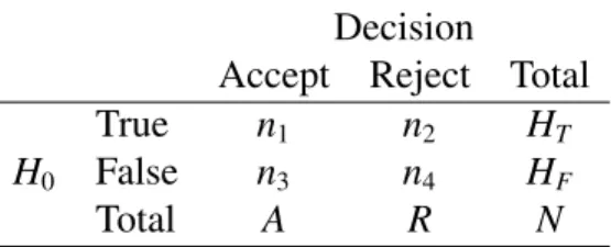
Decision
Accept Reject Total True n1 n2 HT H0 False n3 n4 HF
Total A R N
Table 1.2: Outcomes from N Simultaneous Hypothesis Tests, wheren1+n4 is the total number
of correct decisions,n2 is the number of type I errors, andn3is the number of type II errors.
for the gene-specific variances based on the James-Stein estimator.
A second aspect of particular importance in microarray studies is how to adjust for multiple hypothesis testing. Microarray experiments measure the expression of thousands of genes at once, yet the number of arrays hybridized is typically small. This is the inverse of the usual statistical analysis, where only a small number of hypotheses are examined, and numerous replications are used to achieve accuracy. Thus, traditional methods of adjusting for multiple testing may not be suitable for microarray data. Assuming thatN simultaneous hypothesis tests are being conducted with an desired overall type I error rate of α, the outcomes may be conceptualized as shown in Table 1.2. Traditionally, adjustment for multiple hypothesis testing has been accomplished by controlling the family-wise error rate (FWER; Dudoitet al., 2002). This rate is computed as
FW ER= Pr(n2 ≥1) (1.7)
Thus, the family-wise error rate (FWER) is the probability of one or more type I errors (or false positives) among all genes declared differentially expressed. The FWER is controlled by con-ducting the N individual tests at lower significance level so that the overall level remains atα. The prototypical example is the Bonferroni procedure, which adjusts the level of the individual tests to beα/N. Less conservative methods of adjusting the FWER have also been developed.
Benjamini and Hochberg (1995) proposed an alternative to the FWER, which they call the
false discovery rate (FDR). The false discovery rate (FDR) represents the expected proportion of false positives among all of the rejected null hypotheses (false discoveries) times the probability
of at least one rejected null hypothesis. This is computed as FDR= E n 2 R |R> 0 ×Pr(R> 0) (1.8)
The FDR is generally a more meaningful method of controlling error rates for microarray studies, which are exploratory in nature and so a small number of false positives is acceptable. It also has the practical interpretation that 100αpercent of the genes declared differentially expressed would be false positives. The FDR controlling procedure may be expressed algorithmically as follows: LetNbe the number of null hypotheses, withHT of these being true andHF of these being false.
Let H1,H2, . . . ,HN represent the null hypotheses corresponding to the vector of test statistics
T1,T2, . . . ,TN. Denote the associatedp-values as p1,p2, . . . ,pN so that pi = 1−FHi(Ti) for the
cumulative distribution function (CDF) F(·) under the null hypothesis Hi. Let p(1),p(2), . . . ,p(N)
be the orderedp-values, and letH(i)be the hypothesis corresponding to p(i). Define
j=max i: p(i) ≤ i Nq (1.9)
Then, for independent test statistics and for any configuration of false null hypotheses, rejecting
allH(i),i= 1,2, . . . , j,controls the FDR at levelq.
The above procedure (hereafter called the Benjamini-Hochberg procedure) assumes that theN
null hypotheses are independent, which would seem to be an untenable assumption for microarray studies (Dudoit et al., 2002). However, the proof of the associated theorem does not require independence, and it is possible that this assumption may be relaxed. Benjamini and Yekutieli (2001) showed that the above result for the Benjamini-Hochberg procedure holds under more general conditions for multivariate normal test statistics. Reiner et al. (2003) note that these results for FDR control with one-sided tests apply to microarray experiments; assuming that up- and down-regulation are equally likely to occur, these results extend to two-sided tests as well (Yekutieli, 2002). Benjamini and Yekutieli (2001) further generalize the FDR controlling procedure to allow for arbitrary dependency structures, but this result comes with a considerable
loss of power compared to the Benjamini-Hochberg procedure and is not necessary for most studies (Reineret al., 2003).
1.7
Mixed E
ff
ects Models for Microarrays
1.7.1
Introduction
Kerr, Martin, and Churchill (2000) were the first to propose the use of ANOVA models to adjust for the multiple sources of variation in microarray data. Their original formulation, which is for cDNA microarrays rather than Affymetrix GeneChips, models the log-transformed intensityyof themthmicroarray,dth dye,cthcondition (labeled asvarietyin the original paper), andgthgene as
ycmdg = µ+ Mm+Dd+Cc+Gg+(MG)mg+(CG)cg+εcmdg (1.10)
whereµis the overall mean,Mis the array effect,Dis the dye effect,Cis the effect of condition,G
is the gene effect, (MG) is the array by gene interaction, (CG) is the condition by gene interaction. In the vector and matrix formulations of the model described in subsequent sections, these effects would be incorporated into the design vector (or matrix), denoted x (or X), and the vector (or matrix) of coefficients, denoted β. The error terms ε are assumed to be iid N0, σ2. For this model, the effects of interest are the condition by gene interactions (CG). A nonzero value of this term would be interpreted as differences in intensity across conditions for geneg, indicating differential expression. Although replicates were not explicitly incorporated into the description by Kerr and colleagues, the flexibility of the ANOVA model allows such information to be added easily.
Wolfingeret al.(2001) extended this model for cDNA arrays to include random effects. They divide the analysis into two interconnected ANOVA models. The first is a “normalization” model corresponds to the normalization step in expression summary measures, correcting for systematic differences among arrays to allow valid comparisons. For this model, the log-transformed inten-sityyof thecthcondition (labeled astreatmentin the original paper),mthmicroarray, andgth gene
may be written as
ycmg =µ+Cc+Mm+(C M)cm+εcmg (1.11)
whereµis the overall mean,Cis the condition effect, Mis the array effect, (C M) is the array by condition interaction, andε represents random error. The effects M, (C M), and εare assumed to be normally distributed random variables with mean 0 and variances of σ2M, σC M2 , and σ2ε respectively. These random variables are also assumed to be independent of each other. Wolfinger
et al.did not include dye effects in Equation (1.11) as dye effects were confounded with treatment effects in their experiment. However, dye effects may be added to the normalization model when permitted by the experimental design. The residuals ˆεfrom Equation (1.11) contain the remaining variation after adjusting for treatment and array effects. These residuals are used as the dependent variables in the second “gene” model, which is given by
ˆ
εcmg =Gg+(CG)cg+(MG)mg+ψcmg (1.12)