Projection pursuit methods for exploratory supervised classification

2003

Projection pursuit methods for exploratory

supervised classification

Eun-kyung Lee

Follow this and additional works at:

https://lib.dr.iastate.edu/rtd

Part of the

Biostatistics Commons, and the

Genetics Commons

This Dissertation is brought to you for free and open access by the Iowa State University Capstones, Theses and Dissertations at Iowa State University Digital Repository. It has been accepted for inclusion in Retrospective Theses and Dissertations by an authorized administrator of Iowa State University Digital Repository. For more information, please [email protected].

Recommended Citation

Lee, Eun-kyung, "Projection pursuit methods for exploratory supervised classification " (2003).Retrospective Theses and Dissertations. 1441.

exploratory supervised classification

by

Eun-kyung Lee

A dissertation submitted to the graduate faculty in partial fulfillment of the requirements for the degree of

DOCTOR OF PHILOSOPHY

Major: Statistics

Program of Study Committee: Dianne Cook, Major Professor

Julie Dickerson Heike Hofmann Kenneth Koehler

Huaiqing Wu

Iowa State University Ames, Iowa

2003

UMI

UMI Microform 3105084

Copyright 2003 by ProQuest Information and Learning Company. All rights reserved. This microform edition is protected against

unauthorized copying under Title 17, United States Code.

ProQuest Information and Learning Company 300 North Zeeb Road

P.O. Box 1346 Ann Arbor, Ml 48106-1346

Graduate College Iowa State University

This is to certify that the doctoral dissertation of Eun-kyung Lee

has met the dissertation requirements of Iowa State University

Major Professor

For the Major Program

Signature was redacted for privacy.

TABLE OF CONTENTS

NOTATION GLOSSARY v

1 INTRODUCTION 1

1.1 Scope of thesis 1

1.2 Exploratory methods - Data mining 3

1.3 Projection pursuit 4

1.3.1 Relationship of projection pursuit to other multivariate methodologies 5

1.3.2 Variations of projection pursuit method 7

1.3.3 Projection pursuit indices 8

1.4 Optimization methods used for projection pursuit • 9

1.5 Linear discriminant analysis and its extensions 11

References 12

2 PROJECTION PURSUIT FOR EXPLORATORY SUPERVISED CLASSIFI­

CATION 14

Abstract 14

2.1 Introduction 14

2.2 Index definition 16

2.2.1 LDA projection pursuit index 16

2.2.2 LDA extended projection pursuit index using Lr-norm 21

2.3 Optimization 25

2.4 Assessing certainty in estimating projection 26

2.5 Application 28

2.5.1 Datasets 28

2.5.2 Results 29

2.6 Discussion 32

References 35 3 PROJECTION PURSUIT FOR SMALL SAMPLE SIZE WITH A LARGE NUM­

BER OF VARIABLES 37

Abstract 37

3.1 Introduction 37

3.2 Problems of high dimensionality 38

3.2.1 The capacity of a separating plane 38

3.2.2 The covariance matrix estimation effect 42

3.3 PDA projection pursuit index 43

3.3.1 Index definition 43

3.4 Example 48

3.5 Application : Gene selection 50

3.4.1 Two class case 50

3.4.2 Three class case 55

3.6 Discussion 57

References 57

4 ClassPP : PROJECTION PURSUIT PACKAGE FOR SUPERVISED CLASSI­

FICATION 59 4.1 Introduction 59 4.2 Functions 59 4.3 How to use 60 4.3 Manual 62 ClassPP 62 PPindex.class 63 PP.optimize 64 PP.Tree 66 PP.classify 68 References 70 5 GENERAL DISCUSSION 71

NOTATION GLOSSARY

Xij the jth observation of the ith class,

i = 1,2, ,g and j = 1,2, ,m

B the between group sums of squares

W the within group sums of squares

$ the corrected total sums of cross product

Br the between group difference measured by LR norm

Wr the within group difference measured by LR norm

A the p x k projection matrix

I L D A { A ) LDA projection pursuit index

I L „ { A ) LR projection pursuit index

I P D A ( A ) PDA projection pursuit index

1 INTRODUCTION

1.1 Scope of thesis

Projection pursuit is an exploratory statistical technique for finding projections of multivariate data that reveal interesting structure. Very few projection pursuit methods incorporate class information in the calculation. Therefore they cannot be adequately applied to supervised classification problems. This thesis involves research into projection pursuit methods for exploratory supervised classification problems.

This thesis is a collection of two papers and one software : "Projection pursuit for exploratory supervised classification", "Projection pursuit for small sample size with a large number of variables", and "ClassPP R library".

1. Projection pursuit for exploratory supervised classification

We propose two new projection pursuit indices that incorporate class information and use simulated annealing optimization to find maxima.

• LDA index : the extension of Fisher's linear discriminant analysis

where Xy is the ^-dimensional jth observation of the ith class, i — 1,. . . ,g (number of classes) and j = 1,rii, and A is a p x k projection matrix, and

B = -X.y

1 = 1

w = ^Y)Xij-Xj(Xj,-Xjr

1=1 j-1

k g

Br = Iyu - y..i\r

l — 1 i = 1

w r = X X X \ y i j i - V i . i \r • l—l t=l j=l

• Simulated Annealing Optimization

The purpose of projection pursuit optimization is to find all interesting projections, not only to find one global maximum. Therefore it needs to be flexible to find global and local maxima. We use a modified simulated annealing algorithm.

2. Projection pursuit for small sample size with a large number of variables : application to gene expression data

We discuss how the sample size and the dimensionality are related and how they affect multivariate data analysis from an EDA point of view. Then, we propose a PDA projection pursuit index.

• PDA index : the extension of penalized discriminant analysis

T ,A n _ i _ [ AT( ( 1 — A)W + A • n • I)A|

P ' |Ar((l — A)(W + B) + A • n • I)A| where A is a predetermined parameter and n = Y^i=i n

«-To explore the small sample with a large numnber of variables, LDA and PDA indices are are applied to gene expression data where the sample size is 72 and the number of variables is 3571. A guideline to select genes is provided.

3. Software : ClassPP R package, GGobi implementation

We created the ClassPP library, using the R language, to evaluate and optimize the projection pursuit index functions. This library is available at http://www.public.iastate.edu/~kyung/ClassPP.home.html and will be submitted to the Comprehensive R Archive Network (CRAN). These indices will be im­ plemented into GGobi, providing a tool for exploratory data analysis and data mining (available at http://www.ggobi.org).

1.2 Exploratory methods - Data mining

The initial stage of data analysis is often exploratory. Exploratory data analysis (EDA) provides the first contact with data and it also serves to reveal unexpected departures from familiar models. EDA is for clarifying the structure of the data and getting ideas for a more sophisticated analysis of a scientific problem. The techniques of exploratory data analysis consist of a number of informal steps including checking the quality of the data, calculating simple summary statistics and constructing appropriate graphs. Also emphasis is on visual displays that have been a major contribution of EDA.

EDA and data mining are similar except the size of data. Data mining is usually connected with huge databases and deals with a large number of variables. It is one part of the process of knowledge discovery in databases. Classification (supervised classification) and clustering (unsupervised classification) are commonly used. After applying data mining methods, the discovered patterns need to be interpreted and assessed for their potential use in prediction in test data. Accuracy, how well the pattern predicts in data is still the main concern in data mining, but increasingly interpretation is important also. Ideally, relatively simple and interpretable models are used instead of complex models.

Visualization methods can assist both interpretation and accuracy. Because visualization is usually concerned with exploring data and information graphically, as a mean of gaining understanding and insight into data, it can be helpful to interprété and assess the fitted model.

EDA and data mining both can help reveal patterns and features of the data corresponding to patterns. However, there is a problem. If we look hard enough within a large data set, we tend to find spurious relationships. This is called data snooping. One example can be found in Crack(1999) on a financial data analysis. Data snooping happens when we find statistically significant but spurious relationships between empirical data. To prevent this problem, model fitting should be limited to the training set. If we use the whole dataset including the test set to find patterns of data, we tend to overestimate. To use simple models instead of complicated models is also another way to escape this problem.

Multivariate data sets in which several numerical variables are recorded for each individual, are fundamental in most studies. Classical multivariate analysis methods usually use a variance-covariance matrix to evaluate the relationship of variables under the Gaussian assumption. Sometimes, they need to sphere the data before applying the method of analysis. If some variables are highly correlated in the data, we need to remove this collinearity first, for example, remove some variables or reduce the dimensionality that data points are independently distributed.

increases, the number of possible locations in a multivariate space increase exponentially. It means that high-dimensional space is mostly empty and for multivariate Gaussian distribution, the large probability lies far-from the center in high-dimensional space. Therefore most of multivariate analysis methods are inadequate.

In EDA point of view, the first step in data analysis is to look at the data. As EDA techniques expand toward multivariate and large data set , the role of graphical technique has begun to increase. However, in high-dimensional data, it is very difficult to present useful information by pictures that are restricted to be in low-dimensions (usually 2-3 dimensions). Projection pursuit approach can give us a solution to solve this problem.

1.3 Projection pursuit

To find a projection from the high-dimensional space into the low-dimensional space is one-way to escape dimensionality problems. Projection of the data generally implies loss of information and perhaps it can introduce some distortion of data. Therefore the projection should be carefully chosen, then the amount of information loss can be minimized.

Projection pursuit is a technique developed for obtaining low-dimensional linear projections of mul­ tivariate data. The term "projection pursuit" was first used by Friedman and Tukey (1974) for a technique of the exploratory analysis of multivariate data. It is for finding the low-dimensional linear projections which reveal interesting structure. This low-dimensional projection is found by optimizing some pre-defined criterion function, called a projection pursuit index.

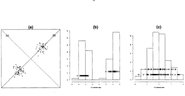
The basic question in projection pursuit is to define what projections are interesting. It is usually argued that the Gaussian distribution is the least interesting one, and the most interesting projections are the ones revealing multi-modal distribution or cluster structure. (Figure 1.1)

Interesting multivariate structure usually does not show up in all projections, and no single pro­ jection might contain all the information. Therefore it is important to choose a set of projections in the projection pursuit method. Also the projection pursuit algorithm can be applied to each cluster separately and find new projections that may reveal further clustering within each separated data set. The main advantage of the projection pursuit method is to bypass the curse of dimensionality by working in the low-dimensional linear projections. It also can ignore nuisance variables. This is a distinct advantage over methods based on interpoint distances like minimal spanning trees, multidi­ mensional scaling and most clustering techniques. Even though these methods also can avoid the curse of dimensionality, all of them can be derailed by nuisance variables.

Figure 1.1 (a) 2-dimensional data with 2 classes, (b) The histogram of the most interesting ID projected data, (c) The histogram of the least interesting ID projected data.

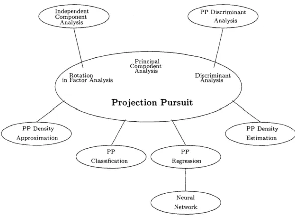
1.3.1 Relationship of projection pursuit to other multivariate methodologies

Principal components analysis is a familiar exploratory technique of this kind. It is a special case of the projection pursuit method in which the index of interestingness is the proportion of total variance accounted for by the projected data (7(a) = a'Sa, where S is the variance-covariance matrix of data and a is a projection.). When projection pursuit is used for exploratory data analysis, we usually compute a couple of the most interesting 1-dimensional projection sequentially, that is, after finding the most interesting 1-dimensional projection, find another most interesting 1-dimensional projection that is orthonormal to the first one, and continue this. Some structure of the data can be visualized by showing the distribution of the data in the 1-dimensional subspaces, or on 2-dimensional planes spanned by two of the 1-dimensional projection pursuit direction. This method is an extension of the classical method of using PCA for visualization, in which the direction of the data is shown on the plane spanned by the first two principal components.

Thus principal component analysis extracts scale effects. One of the goals of projection pursuit is to discover additional structure not captured by the correlational structure of the data. A way to ensure this is to make the projection index invariant to all nonsingular affine transformations in the ^-dimensional data space (Huber, 1985).

Sphering provides a convenient way to construct an affine invariant projection pursuit index. Spher­ ing is to perform a linear transformation that removes all of the location, scale, and correlational structure. All linear combinations after sphering have zero mean, unit variance, and zero correlations.

It is analogous to carry out principal components analysis on the centered data. However, sphering has an unfortunate side effect. Sphering is graphically distracting because it changes the shape of the data and may in some cases hide features that were previously visible (Cook, et al,1995).

Fisher's linear discriminant analysis (LDA) is to find the linear combination such that the between-group variance is maximized relative to the within-between-group variance. Let {Xgn : g = 1, • • • , G, and n = 1, • • • , rig} be a sample, where Xgn is the nth ^-dimensional observation in group g. Let

a

B = X ni(Xj. — X..)(Xj. — X..)T : sample between iroups matrix

i=i g ru

W = X - Xi.)(Xy - Xj.)T : sample within groups matrix

1=1 j=l

where X«. = ^ YJjU xu> X . = ± ELi E"Li xv a nd N = ELi

%-Let Ai, • • • Xp be the eigenvalues of W_1B, and e%, - - , ep be the corresponding eigenvectors. Then

aTBa ifBh x ,

«Two - (Twfi - ^

and /fX is the first linear discriminant. Similarly, we can find the second linear discriminant ZjfX by

arBa ljBl2 4 ,

= iTwg = A. , b = ^

Continuing, Z^X = e^X is the /cth linear discriminant. In this point of view, LDA is a special case of projection pursuit methods which finds set of orthogonal projections onto one-dimensional space sequentially.

Multivariate data are often viewed as multivariate indirect measurements arising from underlying sources, which typically cannot be directly measured. Factor analysis is a classical technique that aims to identify these latent sources. Factor analysis models typically have the assumption of Gaussian distribution. Recently, Independent Component Analysis (ICA) has emerged as a strong competitor to factor analysis. It deals with the non-Gaussian nature of the underlying sources.

ICA comes from the blind source separation problem. The goal of the blind source separation is to recover independent sources given only sensor observations that are linear mixtures of independent source signals. ICA provides a way to find a linear coordinate system such that the resulting signals are as statistically independent from each other as possible. In contrast to correlation-based transformations such as principal component analysis, ICA not only decorrelates the signals but also reduces high-order

statistical dependencies.

The ICA model has exactly the same form as Factor analysis, except the factors are assumed to be non-Gaussian and statistically independent. ICA starts from a factor analysis solution, and looks for rotations that lead to independent components. From this point of view, ICA is just another factor rotation method. Projection pursuit is usually performed by finding the most non-normal projections of the data. This means that all the non-normality measures and the corresponding ICA algorithms could be also called projection pursuit indices and algorithms.(Lee, 1998; Hastie, et al.,2001)

1.3.2 Variations of projection pursuit method

Most of the nonparametric estimation techniques (kernel, nearest-neighbor, and spline smoothing) are based on local averaging. In high-dimensional space, they do not perform well unless the sample size is very large. Friedman and Stuetzle (1981) suggested the projection pursuit regression (PPR), which combines nonparametric regression in high-dimensional data with the projection pursuit method.

PP Density Approximation PP Density Estimation Classification Neural Network Independent Component Analysis Rotation in Factor Analysis

Projection Pui

PPR model has the additive form /(X ) = f o ( X ) + Em=i 9 m ( a m X ) > where f o ( X ) is a initial model, usually y, and uses iterative method to estimate this model. In each iteration, estimate the regression function gm using residuals of previous iteration as response variable and a projected data a^X as

predictor variables, and continue these procedure until the residuals have no information. In here, am is selected for maximizing R2 in each regression and local averaging is used to estimate gm. The

projection pursuit regression model has not been widely used in the Statistics arena. But it plays an important role in the neural network arena, which is a widely used data mining procedure. The single hidden layer back-proparation network, which is the most widely used neural net, is a two-stage classification or regression model and can be explained as PPR model.

The projection pursuit density estimation (PPDE : Friedman, et al (1984)) is also used for solving the problem of local averaging in high-dimensionial space in an iterative manner. The PPDE method constructs estimates of the form PM(X) = po(X) Hm=i FMIA^X), where po(X) is an initial multivariate density, usually a normal distribution, am is a projection and fm is an augmenting function, the ratio

of two marginal distributions of pm-i(X) and p{X). In each iteration, find am that maximizes the

cross-entropy and update fm until the augmenting function fm has no pattern.

Posse(1992) suggested the projection pursuit discriminant analysis (PPDA) for two groups. He used kernel estimation of the projected data instead of the original data and used the total probability of misclassification of the projected data as the projection pursuit index. Polzehl(1994) extended Posse's PPDA. He considered the cost of misclassification and used the expected overall loss as the projection pursuit index. In addition, there are many other applications using the projection pursuit method, such as projection pursuit classification and projection pursuit density approximation (Huber, 1985).

1.3.3 Projection pursuit indices

Friedman and Tukey's index(1974) used interpoint distances as well as the measure of the spread of data in robust manner. 1(a) = s(a)d(a), where a is a projection, s(a) is the trimmed standard deviation, and d(a) is the local density. Jones and Sibson(1987) showed that d(a) is an estimate of f f2(z)dz (order-2 entropy), where / is the density of data which is projected onto a and considered

the order-1 entropy, — f /log/. The standard normal density minimizes this, which means this index measures deviation from normal density.

They also suggested the moment index, (k32 + j K4 2) / 1 2 , where Kg and «4 are cumulants. This index

was made to avoid reference back to the original data at each step of the numerical procedure. However, the moment index dramatically emphasizes departure from normality in the tails of the distribution.

In Friedman and Tukey's index and the entropy index, kernel estimation is used to estimate /. Friedman(1987) revisited exploratory projection pursuit and proposed an index estimating L2 dis­ tance between the density of the projected data and the standard normal density. To emphasize de­ partures from normal in the main body of the distribution instead of in the tails, he used a trans­ formation, Y = 2$(%) — 1, where $(%) is the standard normal cdf. Friedman's Legendre index is IL — (g(y) — i)2 dy. This index is named after Legendre polynomial which is used to estimate

This Legendre index generated much discussion. Hall(1989) proposed the Hermite index IH =

f {f(x) - <fi(x)}2 dx, where 0(x) is the standard normal pdf, and used the Hermite polynomial to

estimate /. Using the inverse transformation, Cook, et al. (1993) made the Legendre index to the same form of the Hermite index, IL = f {/(x) — (f>{x)}2 2tp(x)^'-E, and indicated that the Legendre index upweights in the tails, exactly the opposite of Friedman's intension. They suggested the Natural Hermite index, IN = f (f(x) - <j>(x)}2 <j>(x)dx. It is natural because the distance from the normal density is

taken with respect to Normal measure. They also used a Hermite polynomial. Low-order of Hermite and Natural Hermite indices often find projections with a hole in the center and low-order of Legendre index tends to find projections containing skewness. Higher indices become short sighted and find details.

1.4 Optimization methods used for projection pursuit

Optimization procedures play an important role in projection pursuit methods. In most optimization problem, the global maxima is required and local maxima are useless. On the other hand, the purpose of projection pursuit optimization is to find all interesting projections, not only to find one global maximum, because sometimes the local maximum can reveal unexpectedly interesting data structure. For this reason, the projection pursuit optimization algorithm needs to be flexible to find global and local maxima.

In the beginning of the projection pursuit research, the projection pursuit indices were smooth and the Rosenbrock and Powell principal axis search algorithms, sophisticated hill-climbing algorithms, have been sucessfully applied without enountering any instability (Friedman and Tukey, 1974). Friedman and Stuetzel (1981) modified the Rosenbrock method to search on the unit sphere. This method is started at the best coordinate direction. Because there is no guarantee that the global optimum will be found, the search is restarted at ramdom directions if the local optimum is not acceptable. This prevents from premature termination.

Projection Pursuit index and method Optimization procedure Friedman and Tukey('74) 1 ( a ) = s ( a ) d ( a ) s(a) : trimmed s.d.

d(a) : local density

- robust to the outliers

Rosenbrock

Powell principal axes

Friedman and Stuetzl('81)

PP Regression

1(a) = 1 E'=l(^I5°("'*,))2

Sa(a'xi) : regression function

Ti : residual of previous iteration

Rosenbrock method

- modified to search on the unit sphere

Jones and Sibson('87)

1 ( a ) — f /log / : entropy index

1(a) = K3+4K4 : moment index

- emphasize the tail area

hill-climbing method steepest-slope methods - solution are too local Friedman('87) jL(q) = /-i (ff(y) -

\)

: Legendreindex - upweight in the tails

hybrid optimization strategy - solutions are too local

Hall('89) IH( a ) = f { f ( x ) - 4 > ( x ) }2 d x

: Hermite index

Crawford('91) genetic optimizer

Posse('92) PP Discriminant Analysis random search

Cook, et al('93) IN( a ) = f { / ( x ) - ( j > ( x ) }2 c f > ( x ) d x

: Natural Hermite index

Pozehl('94) PP Discriminant Analysis a combination of stochastic search

and the simplex algorithm

Cook, et al('95) interpolation tour

simulated annealing

Table 1.1 Summary of projection pursuit methods and optimization procedures

Later, Jones and Sibson (1987) used a steepest-ascent algorithm and Friedman (1987) modified this algorithm with a simple stepping search to determine a region of interest. It is called a hybrid optimization strategy. However these methods find solutions too locally and a solution is not interesting if the starting point is not in the attractive domain. In 1991, Crawford suggested the genetic optimizer.

It is similar to the gradient-based method using a large number of random starts.

Posse (1990) pointed out the problems of the former optimization procedures and suggested a random search for finding the global maximum of a projection pursuit index. It is an extension of Ruber's method (1987) to the 2-dimensional case. He used this method for PPDA. Polzehl (1994) used a combination of a stochastic search and the simplex algorithm. Cook, et al (1995) suggested an interpolation tour for a grand tour and simulated annealing for optimizing projection pursuit indices.

1.5 Linear discriminant analysis and its extensions

In the previous section, we mentioned that LDA can be explained as projection pursuit method. We look at LDA in a different way. LDA starts from the assumption that the data of each group come from Gaussian distribution with different means(^9) and same variance-covariance matrix(S). Therefore the linear discriminant functions are

Mx) = xT£~Vs

-If we change the common variance-covariance assumption to non-homogeneous variance-covariance across groups, the discriminant functions changes to a quadratic form(QDA)

Mx) = ~2 'og - 2^X ~ ~ A1

»)-LDA and QDA work very well in most cases because the data can only support simple decision boundaries such as linear or quadratics, and the estimates provided via the Gaussian models are stable. But QDA has a serious drawback. For large p, we need to estimate too many parameters, (G — 1) x p{p + 2 ) / 2 .

Regularized discriminant analysis(RDA) is a compromise between LDA and QDA. In RDA, the regularized covariance matrix Ëg(a) = aÊg + (1 — a)Ê is used, a can be chosen by cross-validation.

The regulaized covariance matrix can be modified as Êg(a) — aÊ + (1 — a)â2l. As a is decreased, this

covariance matrix is shrunk toward the scalar covariances and the assumption of this analysis can be changed to independent variables (Hastie et al, 2001).

Flexible discriminant analysis (FDA) applies basis expansions to LDA and makes LDA more flexible. Therefore FDA amounts to LDA in an enlarged space. Generalized optimal scoring were introduced to solve FDA. It changed FDA to regression analysis. Sometimes, if this enlarged space is too large, it

creates problem for fitting the model and needs to be regulated. Penalized discriminant analysis(PDA) is proposed to handle this problem. PDA fits an LDA model, but penalizes its coefficients to be smooth. From a regression point of view, PDA can be explained as ridge regression (Hastie et al, 2001). For detailed theoretical descriptions, see Appendix A.

References

Cabrera, J. and Cook, D. (1992). "Projection Pursuit Indices based on Fractal Dimension." Computing Science and Statistics, 17, 474-477.

Cheng, B. and Titterington, D. M. (1994). "Neural Networks : A Review from a Statistical Perspective." Statistical Science,9, 2-54.

Cook, D., Buja, A., and Cabrera, J. (1993). "Projection Pursuit Indexes Based on Orthogonal Function Expansions." Journal of Computational and Graphical Statistics, 2, 225-250. Cook, D., Buja, A., Cabrera, J., and Hurley, C. (1995). "Grand Tour and Projection Pursuit."

Journal of Computational and Graphical Statistics, 4, 155-172.

Crack, Timothy F. (1999). "A Classic Case of "Data Snooping" for Classroom Discussion" Journal of Financial Education, 92-97.

Diaconis, P., and Freedman, D. (1984). "Asymptotics of Graphical Projection Pursuit." The Annals of Statistics, 12, 793-815.

Friedman, J. H. (1977). "A Recursive Partitioning Decision Rule for Nonparametric Classification." IEEE Transactions on Computers, 26 , 404-408.

Friedman, J. H. (1987). "Exploratory Projection Pursuit." Journal of the American Statistical Association, 82 , 249-266.

Friedman, J. H., and Stuetzle, W. (1981). "Projection Pursuit Regression." Journal of the American Statistical Association , 76 , 817-823.

10] Friedman, J. H., and Stuetzle, W. (1982). "Projection Pursuit Methods for Data Analysis." Modern data analysis , 123-147.

11] Friedman, J. H., Stuetzle, W., and Schroeder, A. (1984). "Projection Pursuit Density Estimation." Journal of the American Statistical Association , 79 , 599-608.

12] Friedman, J. H., and Tukey, J. W. (1974). "A Projection Pursuit Algorithm for Exploratory Data Analysis." IEEE Transactions on Computers, C-23 , 881-890.

13] Glymour, C., Madigan, D., Pregibon, D., and Smyth, P. (1997). "Statistical Themes and Lessons for Data Mining" Data Mining and Knowledge Discovery, 1 , 11-28.

14] Hall, P. (1989). "On Polynomial-Based Projection Indices for Exploratory Projection Pursuit." The Annals of Statistics, 17, 589-605.

[15] Hastie, T., Tibshirani, R., and Friedman, J. (2001). The Elements of Statistical Learning : Data Mining, Inference, and Prediction, Springer-Verlag, New York.

[16] Huber, P. J. (1985). "Projection Pursuit." (with discussion) The Annals of Statistics, 13, 435-525. [17] Huber, P. J. (1990). "Data Analysis and Projection Pursuit" Technical Report PJH-90-1, MIT. [18] Johnson, R. A., and Wichern, D. W. (1992). Applied Multivariate Statistical Analysis, 3rd edition,

Prentice-Hall, New Jersey.

[19] Jones, M. C., and Sibson, R. (1987). "What is Projection Pursuit?" (with discussion) Journal of the Royal Statistical Society, A, 150, 1-36.

[20] Lee, T. (1998). Independent component analysis : theory and applications,Kluwer Academic Publishers.

[21] Miller, R.A. (1989). "Some consistency results on projection pursuit estimators of location and scale." The Canadian Journal of Statistics, 17, 81-90.

[22] Morton, S. C. (1990). "Interpretable Exploratory Projection Pursuit." Computing Science and Statistical Proceedings of the 22nd Symposium on the Interfere, 470-474.

[23] Polzehl, J. (1995). "Projection pursuit discriminant analysis." Computational statistics and data analysis, 20, 141-157.

[24] Posse, C. (1990). "An Effective Two-dimensional Projection Pursuit Algorithm." Communications in Statistics - Simulation and Computation, 19, 1143-1164.

[25] Posse, C. (1992). "Projection Pursuit Discriminant Analysis for Two Groups." Communications in Statistics - Simulation and Computation, 21, 1-19.

[26] Posse, C. (1995). "Tools for Two-Dimensional Exploratory Projection Pursuit." Journal of Computational and Graphical Statistics, 4, 83-100.

2 PROJECTION PURSUIT FOR EXPLORATORY SUPERVISED

CLASSIFICATION

A paper to be submitted the Journal of Computational and Graphical Statistics

Abstract

In high-dimensional data, one often seeks a few interesting low-dimensional projections which re­ veal important aspects of the data. Projection pursuit is a procedure for searching high-dimensional data for interesting low-dimensional projections via the optimization of a criterion function called the projection pursuit index. Very few projection pursuit indices incorporate class or group information in the calculation, and hence can be adequately applied to supervised classification problems. We intro­ duce new indices derived from linear discriminant analysis that can be used for exploratory supervised classification.

Key Words: Classification; Data mining; Gene expression; Linear discriminant analysis; Microarray

2.1 Introduction

This paper is about methods for finding interesting projections of multivariate data when the obser­ vations belong to one of several known groups. The type of data would be denoted as a ^-dimensional vector Xy that presents the _/'th observation of the z'th class, i = 1 (number of classes) and j = 1,..., ni (number of observations in class i ) . Let X*. — Xy be the ith group mean and

X = i Ei=i be the total mean, where n = Y l i = ini - Interesting projections correspond

to views where there are the biggest differences between the observations from different classes, that is, the classes are clustered in the view. In this paper, the approach to finding interesting projections uses measures of between group variation,relative to within-group variation. These new methods are

important for exploratory data analysis and data mining purposes when the task is to (1) examine the nature of clustering in the space of the data due to class information, and (2) to build a classifier for predicting the class of new data.

Projection pursuit is a method to search for interesting linear projections by optimizing some pre­ determined criterion function, called a projection pursuit index. This idea originated with Kruskal (1969), and Friedman and Tukey (1974) first used the term "projection pursuit" for a technique of the exploratory analysis of multivariate data. It is useful for an initial data analysis, especially when data are in a high dimensional space. The problem of multivariate data is based on "the curse of dimensionality", that is, most of high dimensional space is empty unless the sample size is quite large. Projection pursuit method helps to explore multivariate data in low dimensional but "interesting" spaces. (The definition of "interesting" projection depends on the projection pursuit index).

Many projection pursuit indices have been developed to discover interesting projections from different points of views. Because most low-dimensional projections are approximately normal (Huber, 1985), most projection pursuit indices have focused on non-normality : the entropy index and the moment index (Jones and Sibson, 1987), Legendre index (Friedman, 1987), Hermite index (Hall, 1989), and Natural Hermite index (Cook et al, 1993).

Visual inspection of high dimensional data using projections is helpful to understand data, especially when it combined with dynamic graphics. GGobi is an interactive and dynamic software system for data visualization and the guided tour with projection pursuit indices is implemented in it (Swayne et al, 2003). The holes index and the skewness index in GGobi are helpful in finding projections with a hole in the center and projections containing skewness, respectively(Cook et al, 1993).

Projection pursuit method have been broadly used in statistical applications, even though they are not always specifically described as projection pursuit methods. Many classical multivariate analysis are explained as simple cases of projection pursuit methods, for example, principal component analysis and discriminant analysis, and the quartimax and oblimax methods in factor analysis (Huber, 1985). Independent components analysis(ICA), a variation of principal component analysis, has the same model as factor analysis, except the factors are assumed to be non-normal and statistically independent. From the factor analysis solution, ICA finds projections(rotations) that lead factors to be independent. From this point of view, ICA is also a special case of projection pursuit (Hastie, et al. 2001).

We start from linear discriminant analysis. Discriminant analysis is a well-known classification method. Among the various two approaches to the discriminant analysis, one is to minimize the total probability of misclassification and another is Fisher's method. Posse (1992) suggested the projection

pursuit discriminant analysis (PPDA) for two groups using the first approach. He used kernel estimation of the projected data instead of the original data and used the total probability of misclassification of the projected data as a projection pursuit index. Polzehl (1994) considered the cost of misclassification and used expected overall loss as the projection pursuit index.

We propose exploratory classification tools using new projection pursuit indices that incorporate class information using Fisher's linear discriminant analysis idea, which expand on Ruber's discussion of projection pursuit for classification. These indices are helpful to build understanding about how class structure relates to measured variables and also can provide graphical representation for verifying supervised classification results. For dynamic graphics, these indices are implemented into GGobi.

Section 2.2 introduces the new projection pursuit indices and describes their properties. The opti­ mization method is discussed in section 2.3 and assessing centainty in estimating projection is discussed in section 2.4. In section 2.5, these indices are applied to two gene expression data sets. A discussion follows.

2.2 Index definition

2.2.1 LDA projection pursuit index

The first index is derived from classical linear discriminant analysis (LDA). The approach, first developed by Fisher (1938), finds linear combinations of the data which have large between-group sums of squares relative to within-group sums of squares. (For detailed explanations, see Johnson et al., 1992.) Let

9

B = Ynjfri. ~ X..)(Xj. - X,.)T : between-group sums of squares, ï— 1

9 ni

W = ^ ^(Xjj - Xj.)(Xy - X,.)T : within-group sums of squares. i=l j = 1

Dimension reduction is achieved by finding the linear combinations, a, which maximize JV^a' *^s a

result, we get â% = ex and = ' w^e r e Ai > • • • > As are eigenvalues of W- 1B, e1 ; • • • , e„

are the corresponding eigenvectors, and s = min(g - 1,p). Note that by construction and convention the eigenvectors are orthonormal, that is, ||e|| = 1 and ej[e&' = 0 so a can be considered to be projection vectors. The linear combination âfX is called the first linear discriminant, and generally âj^X produces the fcth linear discriminant when â& = e&. The result is that the data are reduced to at most s dimensions, and this .s-dimensional subspace provides all the necessary information for

LDA. From this perspective, LDA is a special case of projection pursuit methods that finds orthogonal projections onto 1-dimensional spaces, â&, sequentially.

This approach leads to several natural definitions of a projection pursuit index which uses class information. For a 1-dimensional index, use ^ow values correspond to projections which display little class differences, and high values correspond to projections which have large differences between the classes. For an arbitrary-dimensional index consider test statistics used in multivariate analysis of variance (MANOVA). These statistics are based on comparisons between the within-group

|W| and between-group sums of squares matrices. The most common statistic is Wilks A* = . ; ' ., that

I W+B| is, the determinant of the within-group sums of squares divided by the determinant of the total sums of squares. This quantity also ranges between 0 and 1, although the interpretation of numerical values are reversed from the 1-dimensional measure defined above: small values of A* correspond to large difference between the classes. This scale needs to be reversed to conform to the projection pursuit convention of maximum values corresponding to the most interesting projections.

Let A = [ai a2 • • • a&] define a orthonormal projections onto a ^-dimensional space. Because

in projection pursuit the convention is to maximize projection pursuit index, the maximum should correspond to when the groups are most different and minimum should be when the groups are similar. We follow this convention and use negative value of Wilks Lambda and add 1 to keep this index between 0 and 1. Low index values correspond to little difference between classes and high values correspond to large differences between classes. Then the LDA projection pursuit index is

1 - |a^w+b]a| Mat(w + b)a|*o

0 for |AT(W + B)A| =0

When k = 1 the index is —E j = 1( — _ L — - L . T h e n e x t p r o p o s i t i o n q u a n t i f i e s aT(W+B)a ELi £"ii(aTXji-aI'Xi.)

the minimum and maximum values. For simplicity, we denote W + B as #.

Proposition 1. Let rank($) = p , k < min(p, g ) . Then, IL D A { A) =

k p

0 < 1 — Ai < / l d a(A) < 1 — A; < 1

i=l i=p—k+l

where Ai, > A2 > • • • > Ap > 0 : eigenvalues of

ei, e2, • • • , ep : corresponding eigenvectors of $-1/2W$-1/'2, fi, f2, • • • , fp : eigenvectors of

In (2.0.1), the right equality holds when A* = <&_1/2[ep ep_i • • • ep_fc+i] = 3>~1//2[fi f2 • • • ft] and

the left equality holds whenA* = <&~ll2[e,k Bk-\ ei] = 0"^2[fp_t+i fp-fc+2 • • -

fp]-The proof is in the appendix. To simplify the situation, assume that data are sphered. For sphered data, $ = (n — 1)1 and ILDA(A) = 1 - (^-j-)t:|ATWA|. According to Proposition 1, this index has a

maximum value when the projection is A* = [fi • • • f*], where fi, • • • , f<: are eigenvectors of B. This

projection A* can be explained as the first k largest principal components of B, that is, this projection reveals the most spread class mean structure.

Exactly speaking, A* is not an orthonormal projection, but an normalized projection with A*T<1>A* =

I. Therefore, we can find an orthonormal projection A such that the columns of A and A* spans the same space. That is, there exists a nonsingular matrix R&x& such that AR = A*. The columns of A and A* span the same vector space and

IL D A (A * ) = 1 - |A*TWA* |A (

W

B

A

R

A

WAR

R

A

W

B

AR

R

A

WA

R

Therefore, A is the optimal projection that is spanned by A*. Usually R is not unique and we can get different optimal projections whenever we optimize the LDA index, but they represent the same vector space and have same information about linear discriminiant analysis. The difference is just directions. A problem arises for LDA when rank(W) = r < p. We need to remove collinearity before applying LDA by variable selection. Otherwise, we need to modify the W-1 part of the calculation. For example, use the pseudo inverse (pseudo LDA : Fukunaga, 1990) , or use ridge estimate instead of W(regularized discriminant analysis : Friedman, 1989). This is not a problem for the projection pursuit approach unless r < k. In projection pursuit method, we work on /c-dimensional space instead of p-dimensional space. Therefore we can find interesting projections without initial dimension reduction or any other modification.

Proposition 2. Let rank(^) = r < p , k < min(r,g ) . Then, i - n ^ < w A ) < ! - n Si (2.o.2) i = r — k + 1 where $ = _{F Q} A 0 " P T ' A 0 = PAPT 0 0 _ QT P\PT : spectral decomposition of #, P : k x r matrix, PTP = Ir, Q : k x ( k - r ) matrix, QTQ = h -r,

A = diag[<5i, <52, • • • , <5r] : r x r diagonal matrix, 61,62, " , 5r : eigenvalues of A~1/2PTWZPA~1'/2,

ei, e2, • • • ,er : corresponding eigenvectors of A ~l/2PTW P A ~1/2.

In (2.0.2), the right equality holds when A = PA-1/2[er er_i ••• er_t+1], and the left equality

holds when A = PA_1/2[efc e^-i • • • ei].

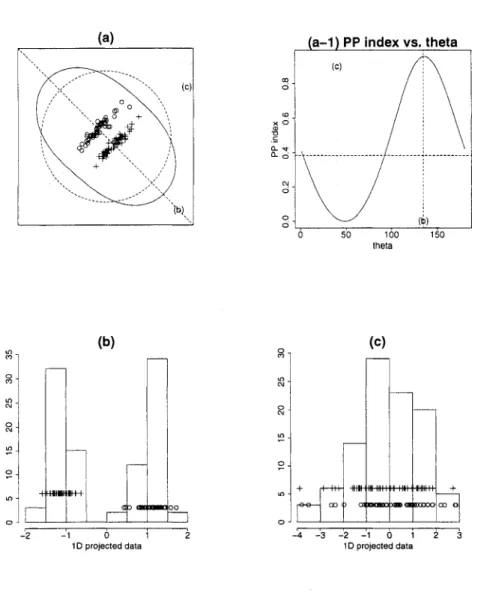
To illustrate the behavior of this index, we use the following type of plot that was introduced by Huber(1990). In one-dimensional projections from 2-dimensional space, for 9 — 0°, • • • , 179°, the projection pursuit index is calculated using projection a@ = (cosd, sin6) and displayed radially as a function of 0. In each figure, the data points are plotted in the center. The solid line represents the index value, ILDA, plotted in relative distances from the center. The dotted circle is a guide line plotted at the median index value. The maximum index value is obtained when the data are projected onto the straight dotted line.

Figure 1 shows how the LDA index works and compares this optimal projection to the first principal component. Data are simulated from two normal distributions with same variance-covariance structure,

( 1 0.95 \ / -1 \ / 1 \

S = , and different means, /xi = and yu2 = . Each group has 50

V 0.95 I ) V 0.6 / \ -0.6 J

samples. Figure 1(a) shows that LDA index function is smooth and has maximum value when the projected data reveals two separated classes, (b) and (c) are the histograms of the optimal projected data using the LDA index and the projected data onto the first principal component. LDA index finds separated class structure. On the other hand, principal component finds the most spread data structure.

(a-1) PP index vs. theta (b) - 1 0 1 2 1D projected data (C) en OODODtintfll BXDOO - 4 - 3 - 2 - 1 0 1 2 3 1D projected data

Figure 1. The bivariate distribution with 2 classes, (a) I L D A; (b) projection that maximize I L D A ; (C) projection

corresponding to first principal component The LDA index works well in general situations, but it has some

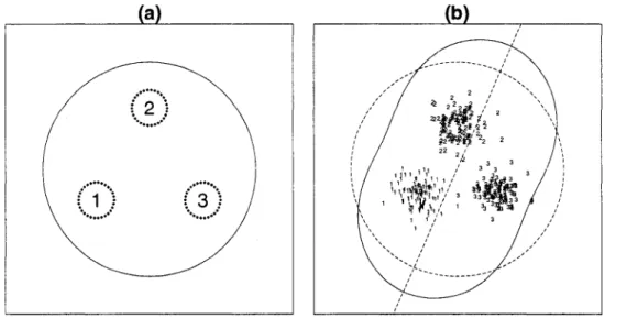
problems under special circumstances. One special situation is 2-dimensional data generated from a uniform mixture of three Gaussian distributions, with unit variance-covariance matrices and centers at the vertices of an equiliterial triangle, Figure 2(a) is the theoretical case where three classes have the exact same variance-covariance matrix and three class means are the vertices of an equiliterial triangle. In this case, all directions have the same LDA index values. In (b) data is generated from a Gaussian distribution with means from the three vertices of an equiliterial triangle and identity variance-covariance matrix. Because of sampling errors, variance structures are slightly different in each class and the three class means don't lie exactly on an equiliterial triangle, then the optimal direction depends

on sampling errors. This is not what we expect from exploratory work. We would like to be able to find all interesting data structures, which in this case would be one of three 1-d projections revealing one group. We extend this problem of LDA index to define a new index that is able to detect interesting structures in this situation.

Figure 2. The bivariate distribution with 3 classes, (a) I L D A •' Theoretical case where the three classes have

the exact same variance covariance structure and the three class means come from the vertices of an equiliterial triangle, (b) ILDA • ' Generated data from three normal distributions with different means and same identity

variance-covariance. Three means come from the vertices of an equiliterial triangle.

2.2.2 LDA extended projection pursuit index using Lr-norm

We start from one-dimensional index. Let y i j = aTXy- be a projected data onto 1-dimensional

space. In LDA index, we use aTBa and aTWa as the measures of between-group and within-group

variations, respectively. These two measures can be explained as the square of Z-2 vector norm.

M

M

aT*a = ~y..f = {||Mys - l„y..||2}2 + {||y - MyJ|2}2 = {||y - 1„Z/..||2}2 ,

i=l j=1

M

yi — [ y n , y i 2 , • • • , V i ng] , and ln = [1,1, • • • , 1]T : n x 1 vector. This total sum of squares $ can be represented as the additive of

B

W.

Br = {||y-Myg||r}r = 53531^-l — 53531^-l j — 1 9 T l i Wr = {||y - iny..\\r}r = 1 2 -i=l j = l m. r-Then 9 ru 9 ni 9 ru TV = {||y - ln2/..||r}r = YlYl\y i = 1 j = 1 i j - y . . \r < Y Y M -y . . \r + Y , Y , \ y i j - y i . \r 1=1 j = l 2=1 j = \

= {l|Myff - l„y..||r}r + {||y - Myfl||r}r = Br + Wr.

Even though the additivity does not hold for LR norm,

B

W

lLr (a) -Br Wr 1/r I|y-Myj|r lly- lnj/..||r ( & . - W 1/r

To prevent this index value from getting too big, we use 1/r power. The one-dimensional LDA index is a special case of this index when r = 2.

For a ^-dimensional projection

A,

Y

A

XY

A.

A

BA =

E E ( m - y . .i)2 E E (jk.i - y . . i ) (2/>.2 - y . .2) E E (Si.2 - v..2) {yi. 1 - 8..1) E E (Si.2 - 5..2)

EE(ft.fc-2/..fc)(5i.i-5..1)

EE(y».i - 2/..1) {yi.k - y..) E E (Si.2 — 5..2) (Si.A: - s..)

and

ArWA =

E E ( y i j i - y i . i )2 E E (y*ji - j/i.i) (yi>2 - y%.2)

E E (yij2 - S i . 2 ) ( y i j i - Ui.i) £ E (y i j 2 - S i . 2 )

E £ {vijk - Vi.k) (2/iji - Si.i)

E E (yiji - Si.i) (y.j/c

E E t e 2 - S 1 . 2 ) { y i j k - s » . E E f e t - y i . k )2

The diagonals of these matrices represent variances of between (or within) group for each variables and off diagonals represent covariances between variables, we take only diagonal parts of these between-group and within-between-group variabilities and extend these sums of squares to LR norms. Let

1=1 i—l j=1 1 = 1

wr = 53 53 (yiii ~ yu^r = 13 tiiYz 1»y..zii'-}r

-1=1 i=l j= 1 /= 1

where Ys; = [ i / i . ; , 2 / 2 . ; , " • , Y , = YU T, Y2iT, • • • , Ygi1

Then,

,and Yjj — [j/ii/jjtoii • • • j Vinsi\

^Lr

(a) =

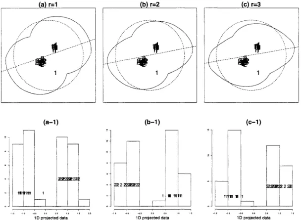
Figure 3. The bivariate distribution with 3 classes(as used for Figure 2-(a)) (a) I Lx (b) I L3 (C) I L5 •' When r=2 and R=4> the index is the same as ILDA, shown in Figure 2(a)

In Figure 3, we can find three optimal projections for each r (r = 1,3,5) and also find different patterns as r changes. When r = 1, all three optimal projections separate one class from the other two classes. When r = 3, the optimal projections separate three classes. With L5 index, we found the same optimal projection as L\ index case but the index function is smoother than L\ index. When r is 2 and 4, this index has the same value for all directions, same as LDA index.

LDA index and LR index (r > 2) are usually sensitive to outliers, mainly due to use distance based

measures. Even though L\ index is based on distances, this index is more robust to outliers than other indices. This comes from the properties of the least absolute value estimator, called L\ estimator. By maximizing Li norm instead of L2 norm, we usually get a robust estimator. The resistance of the

L\ estimators to outliers and their robustness to heavy tailed distributions make this estimator useful

alternatives to the usual least squares (L2) estimators. Although in general the L\ estimators are not unique, they all share this property. (For detailed explanations, see Bloomfield, et al, 1983)

(c) r=3 (b) r=2 (a-1) m u t 2222z22: (b—1 ) (C-1)

1D projected data 1D projected data 1D projected data

Figure 4• The bivariate distribution with 2 classes : class 1 has an outlier (a) ILx (a-1) Histogram of

the projected data onto L i optimal projection (b) IL2 (B-1) Histogram of the projected data onto L2 optimal

Figure 4 shows how these indices work for an outlier. In each plot, there are two classes (1 and 2). The class 1 has 21 observations with one outlier and the class 2 has 20 observations. The histogram of the best one-dimensional projected data using L\ index (Figure 3 (a-1)) shows that the outlier is separated from two groups and the best projection is not affected by this outlier. When r > 2, the best projections are a little bit shifted toward the direction that the class 1 includes this outlier. Except this outlier, L\ index provides a more separable projection than the best projection of Lr{r > 2) index.

2.3 Optimization

A good optimization procedure is an important part of projection pursuit. The purpose of projection pursuit optimization is to find all interesting projections, not only to find one global maximum, because sometimes the local maximum can reveal unexpectedly interesting data structure. For this reason, the projection pursuit optimization algorithm needs to be flexible to find global and local maxima. We use a simulated annealing approach.

Simulated annealing was first proposed by Kirkpatrick et al (1983) as a method to minimize criterion functions that have many variables. The fundamental idea of simulated annealing methods is that a rescaling parameter, called the "temperature", allows control of the speed of convergence to an optimal value, whether the optimal value is global and local. For a criterion function h(8), called the "energy", we start from the initial value do- 0* is generated from a neighborhood of (90. Then, 6* is accepted to a new value with probability p that is defined by temperature and the energy difference between 6>o and 9*. This probability p guards against getting trapped into a local minimun.

For projection pursuit optimization, we use two different temperatures, one (D,) is for neighborhood definition, and the other (T,) is for the probability p . D, is rescaled by the predetermined cooling parameter c and T; is defined by l0j,^°+1) • Before we use this algorithm, we need to choose cooling parameter c and initial temperature To first. The cooling parameter c decides how many iterations is needed to converge to optimal value and whether the optimal value is a local maximum or a global maximum. The initial temperature To also takes part in the speed of convergence. If we use small c, the optimal value can be found in a small number of iterations, but optimal value might be a local maximum. If c is large, we need more iterations to get an optimal value, but this optimal value is the global maximum. Therefore this algorithm is very flexible that we can find the local or global maximum

value.

Simulated Annealing Optimization Algorithm for Projection Pursuit

1. Set initial projection A0, calculate initial projection pursuit index value Io = 7(A0) For ith iteration,

2. Generate a projection A, from NO{ (A0),

where = c\ c is a predetermined cooling parameter in range (0,1),

Net (A0) — {A : A is a orthonormal projection with direction A0 + DiB for all random projections B}.

3. Calculate U = I{Ai), AU - U - I0, = log^0+1),

4. Set A0 = Ai and I0 = Jj with probability p = min^exp , lj and increase i to i+1

Repeat 2-4 until A/j is small.

2.4 Assessing certainty in estimating projection

Because the projection pursuit method usually operates on high dimensional data, it is not easy to check whether the optimal projection is located in the position that represents interesting data structure. This uncertainty comes from the optimization. In our optimization algorithm, we can control this uncertainty with changing the cooling parameter.

1

thela

Figure 5. The bivariate distribution with 4 classes (a) IL! (b) 9 vs. IL1 plot :the dashed line (1) is the global

Figure 5 shows how this optimization works with different cooling parameters. Data in (a) are gen­ erated from four normal distributions with different means, pi = [5,5]T, = [-5, -5]T, ^3 = [3, -3]T, and /U4 = [—3,3]T. Each group has 50 samples, (b) shows L\ index values for 6 = 0°, • • • , 179°. In here Li index function has local maximum(2) and global maximum(l). By changing cooling parameters, we can control the probability of reaching the global maximum or local maximum. This is demonstrated in Figure 6: vertical dotted lines are optimal theta that obtained from 100 time repeated optimization. Numbers on the line shows how many times this optimal theta are found in 100 iterations. As the cooling parameter decreases, the chance to get a local maximum instead of global maximum is higher.

coolinq= 0.7

Figure 6. The bivariate distribution with 4 classes(same as Figure 5) : 9 vs. Li index with different cooling parameters. As cooling parameter is decreased, the chance to get local optimum is increased.

Training set = 100% Training set = 90% Training set = 80%

Figure 7. Optimal ID projection for various size of training sets of Iris data : X and Y axis represent 2D optimal projection for the whole data

The optimal projection largely depends on the data. This might be another source of uncertainty. To check how this projection pursuit method works for data, we use Fisher's Iris data (Fisher, 1938). In Figure 7, points with three different characters show the optimal 2D projected data using LDA index and lines are optimal ID projection vectors from 200 training sets. As training set size is smaller, more variation in the optimal projections is observed .

2.5 Application

DNA Microarray technologies have changed radically and provide a powerful tool for analyzing thousands of genes simultaneously. Comparison of gene expression levels between samples is quite useful to obtain information about important genes and their functions. Because of the large number of genes and a typically small number of samples, analyzing DNA microarray data presents unique challenges to data analysts.

A recent publication (Dudoit et al., 2002) on the comparison of discriminant methods for gene expression data has focused on the classification error. We will use the same data sets to demonstrate the performance of our PP indices.

2.5.1 Datasets

Leukemia This dataset originated from a study of gene expression in two types of acute leukemias,

NCI60 This dataset consists of 8 different sites of cancer origin : 9 cases from breast, 5 cases from

Standardization and Gene Selection The gene expression data were standardized so that the observations have mean 0 and variance 1 across variables. For gene selection, we use the ratio of

between-group to within-group sums of squares.

E L l E L l 1 ( V i = k) (xi J - * k , j )2

where x.j = ^ YH=i xi,j and î&j = ' • ^t the beginning, we follow the original study

(Dudoit et al, 2002) and start with p—40 for the leukemia data and p=30 for the NCI60 data and discuss various numbers of genes later.

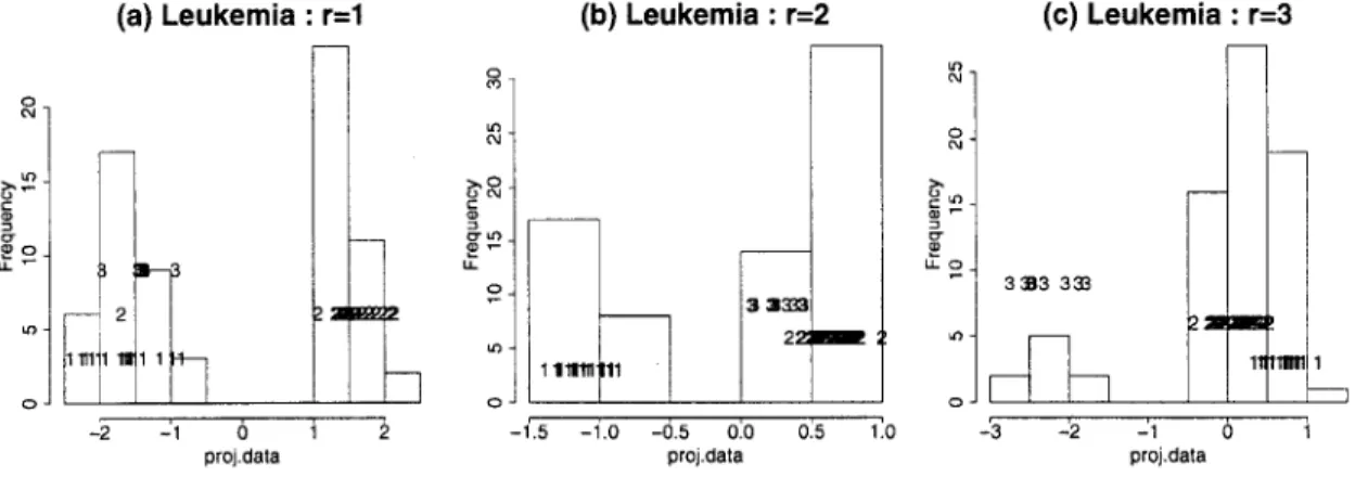
2.5.2 Results ID projection (a) Leukemia : r=1 2 ill wii 1 - 1 0 proj.dala (b) Leukemia : r=2 3 3333 2: -1.0 -0.5 0.0 proj.dala 0.5 (c) Leukemia : r=3 1.0 -3 - 1 0 proj.dala

Figure 8. Leukemia data - ID projection

(p=40)-1: AML 2: B-cell ALL 3 : T-cell ALL

Figure 8 displays the histograms of the projected data onto the optimal ID projections. For this application, we choose very large cooling parameter (0.999) to lead to global maximum. In the Leukemia data, when r=l (Figure 8-a), the B-cell ALL class is separated from the others except one case. When r = 2(Figure 8-b), the result of Lr index is the same as the result of LDA index. In this case, the AML

class is separated from the others. As r is increased, this index tends to separate the T-cell ALL from the others.

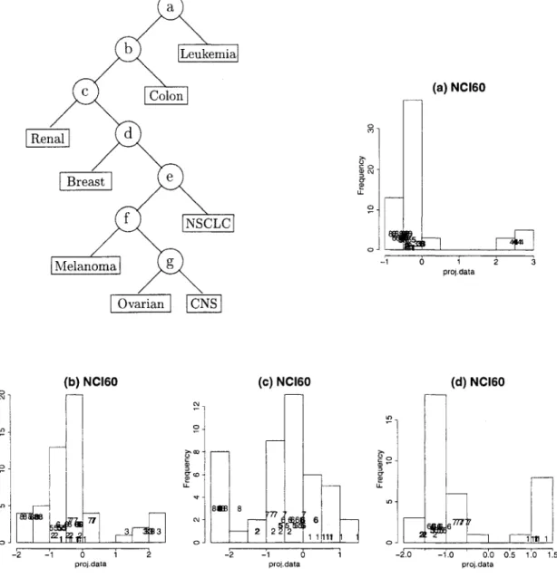
The NCI60 data is a quite challenging example. For such a small number of observations, there are too many classes. For this data, we try the isolation method that applies projection pursuit method iteratively and takes off one class at a time. (Friedman and Tukey, 1974). The 8 classes are too many to

separate in ID at once. After finding one split, we apply projection pursuit in each partition. Usually one class is peeled oif from the others in each step. Figure 9 illustrates how this works. In the first step (9a), we separate Leukemia from the others. At the second step, Colon class is separated (9b). Then, Renal, Breast, NSCLC, Melanoma classes are separated sequentially. Finally, Ovarian and CNS classes are separated. The tree diagram in Figure 9 illustrates the classification splits.

CNS Colon Renal

NSCLC

Figure 9. NCI60 data - ID projection (p=30).

2D projection

(a) Leukemia : LDA (b) Leukemia : r=1 (c) Leukemia : r=2

-1.0 -0.5 0.0 0.5 1.0 1.0 -0.5 0.0 0.5 1.0

Figure 10. Leukemia data - 2D projection (p=40).

1: AML 2: B-cell ALL 3 : T-cell ALL

(a) NCI60 : LDA (b) NCI60 : r=1

CO 3 C O 4 41 (ç) NCI60 : r=2 -4 -3 -2 -1 0 1 -2.0 -1.5 -1.0 -0.5 0.0 0.5

Figure 11. NCI60 - 2D projection (p=30).

1: Breast 2: CNS 3: Colon 4: Leukemia 5: Melanoma 6: NSCLC 7: Ovarian 8: Renal

Figure 10 shows the 2D plots of the projected data onto the best 2D projections for the Leumekia data. All three classes separate easily using the LDA index. Using the Lj index, the B-cell ALL class is separated with one exception (same case of the result of ID projection). In 2D case, the LDA index is usually not the same as Li index unless there is no correlations, that is, B and W are all diagonal matrices. By comparing the results of these two indices, we can see the effect of correlation. In (c),

class means are almost all in one line. On the other hand, when correlation structures in considered (Figure 10-a), class means form the triangle structures. As r is increased, the AML and the B-cell ALL are more close together and the T-cell ALL is separated. In the NCI60 data, Leukemia class is clearly separated from the others for all indices(Figure 11).

In the classification error comparisons (Dudoit et al, 2002), LDA method shows the poor performance to these gene expression data. We focus on Leukemia data investigate this poor performance of LDA method and use same method to assess uncertainty for data. For 100% training sets, the optimal ID projections are in almost same direction and separate AML from the others(Figure 12). As the size of training set is decreasing, optimal projections are quite different and tend to separate T-cell ALL from the others. This can make more misclassifications. The first plot (with 100% training set) can prove the consistency of our optimization method for high dimensional data.

Training set = 100% Training set = 80% Training set = 67%

Figure 12. Optimal ID projection for various size of training sets: Leukemia

2.6 Discussion

We have proposed new projection pursuit indices for exploratory supervised classification and ex­ plored their properties. In most applications, LDA index will work well to separate classes. Sometimes, Lr index with r= 1 finds outliers. For exploratory supervised classification, we need to use all of them

and combine all different results together. These indices can be used for examining class structure in the data space and to find the important variables that play the major roles in separating classes. These are useful when building a classifier and for assessing new classifiers.

have considered the problem of constructing tree-structured classifiers that have linear discriminants at each node. Friedman(1977) reported that applying Fisher's linear discriminants, instead of univariate features, at some internal nodes was useful in building better trees. He treated an G class problem as a series of two-class problems. For each two-class problem, a recursive partitioning is performed to separate one of the class populations from all of the others. We can extend his idea using projection pursuit method. To find an optimal linear split for two classes, ID projection pursuit methods are used with various PP indices that incorporate class information. This is similar approach to isolation method that we applied to NCI 60 data (Figure 8). Using projection pursuit method,