Practice and Retention: A Unifying Analysis

Journal of Experimental Psychology: Learning, Memory, and Cognition 1999, Vol. 25, No. 5,1120-1136

Copyright 1999 by the American Psychological Association, Inc. 0278-7393/99/S3.00

Practice and Retention: A Unifying Analysis

John R. Anderson, Jon M. Fincham, and Scott Douglass

What is the strength of a memory trace that has received various practices at times tj in the past? The strength accumulation equation proposes the following: strength = 2.tj~d, where the summation is over the practices of the trace. This equation predicts both the power law of practice and the power law of retention. This article reports the fits of the predictions of this equation to 5 experiments. Across these experiments, participants received as many as 240 trials of practice distributed over intervals as long as 400 days. The experiments also varied whether participants were just practicing retrieving an item or practicing applying a relatively complex rule. A model based on this equation successfully fit all the data when it was assumed that the passage of psychological time slowed after the experimental session. The strength accumulation equation was compared with other conceptions of the retention function and the relationship of the retention function to the practice function.

This article is concerned with an effort to elucidate the relationship between the effects of practice and the effects of forgetting. At least since Newell and Rosenbloom (1981), the practice function has been commonly (e.g., J. R. Anderson, 1982; Lewis, 1978; Logan, 1988; MacKay, 1982) characterized as a power function. When we plot latency to perform a task as a function of number of trials of practice, latency appears to decrease as a power function of the number of trials. The form of this function is

latency = A + B*P~C,

where A is the asymptotic latency, B is the amount of the latency that can be reduced by practice, P is the number of trials of practice, and c is an exponent that reflects learning rate. Similar power functions may appear for other depen-dent variables (J. R. Anderson, 1995), but the power function relationship has been the most documented in the case of latency.

The forgetting function has also been characterized as a power function at least since Wickelgren (1972; Wixted & Ebbesen, 1991). In a recent survey of the literature, Rubin and Wenzel (1996) identified the power function as one of a number of functions that adequately fit the reported retention data. Most often, in the retention literature, accuracy and not latency is the dependent measure, but J. R. Anderson and

John R. Anderson, Jon M. Fincham, and Scott Douglass, Department of Psychology, Carnegie Mellon University.

This research was supported by Grant SBR-94-21332 from the National Science Foundation. We would like to thank Mike Byrne for his comments on this research. Excel files giving the data and model fits are available by following the Published ACT-R Model link from the adaptive control of thought-rational (ACT-R) home page (http://act.psy.cmu.edu).

Correspondence concerning this article should be addressed to John R. Anderson, Department of Psychology, Carnegie Mellon University, Pittsburgh, Pennsylvania 15213. Electronic mail may be sent to ja+ @cmu.edu.

Schooler (1991) and Schooler and Anderson (1997) have shown that the power function description does extend to latency measures. In this case the predicted function is

latency = A + B*Td,

where T is time between presentation and testing and the exponent d reflects the decay rate.

There have been a number of discussions about whether these functions are really power functions. Heathcote and Mewhort (1995) noted that most efforts to fit power func-tions have ignored the intercept (A) and that when this is included perhaps exponential functions produce a better fit. R. B. Anderson and Tweney (1997) and Myung, Kim, and Pitt (in press) noted that averaging data from exponential functions can result in data that fit power functions better than exponential functions. Rickard (1997) argued that the power law of practice holds at best approximately only for tasks that undergo strategy shift and that it can fit poorly when there is a transition from computation to retrieval. The goal of this article is not to advance the state of understand-ing of the power function fits, although we had to be mindful of these issues in pursuing our goal.

The goal of this article is to elucidate how the retention and practice functions relate to one another and more generally how retention effects and practice effects relate. There has been some discussion in the literature about what the retention functions are like for different degrees of practice (e.g., Bogartz, 1990; Loftus, 1985; Slamecka & McElree, 1983). Also, with respect to latency measures there has been considerable interest in the apparent lack of forgetting at high levels of practice (J. R. Anderson & Fincham, 1994; Schmidt, 1988). Using latency measures in a priming experiment, Grant and Logan (1993) found that priming increased as a power function of practice and then decreased as a power function of delay. It is also the case that studies that advertise themselves as just studies of practice have retention effects built in. These studies typically extend over many days, and there is the day interval between

successive practice sessions. Some of these experiments will also give participants weekends off (e.g., Pirolli & Ander-son, 1985), increasing the retention interval for every 6th day of practice. The research reported here focused on effects of practice separated by various intervals.

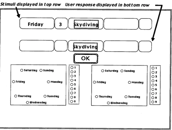
The studies reported here involved a paradigm introduced by J. R. Anderson and Fincham (1994) and continued by Anderson, Fincham, and Douglass (1997). In the first part of these experiments, participants committed to memory eight specific facts such as "Skydiving was practiced on Saturday at 5 p.m. and Monday at 4 p.m." Although participants were not aware of it at the time, they were learning examples of rules about the time relationship between the two events for that sport. In this case, the rule is that the second skydiving event always occurred 2 days later and 1 hr earlier. We call this rule +2, -1. Only after memorizing these examples was the significance of the examples explained to partici-pants, and the participants were then tested with rule-application problems in an interface like that illustrated in Figure 1. Participants were given either the first or second time (day and hour) and had to predict the other time. In the case in Figure 1, where the first time is given as Friday at 3:00 p.m., they would have to predict that the second time was Sunday at 2:00 p.m. They both copied the given elements and made their prediction by clicking the relevant

elements in the boxes below. We were interested in the speed and accuracy with which they could do this. The example in Figure 1 involved going from the first time to the second time, but half of the rules in Anderson and Fincham (1994) required participants to go from the second time to the first time.

Although Figure 1 illustrates a rule trial, in other condi-tions participants were given retrieval trials that are consid-erably simpler. On a retrieval trial, participants were pre-sented with the sport and 2 days or the sport and 2 hr from the original example that they studied and they just had to recall the remaining two (days or hours) from the example. Thus, they might see skydiving, 5 and 4 and had to recall Saturday and Monday. Based on the adaptive control of thought-rational (ACT-R) theory (J. R. Anderson, 1993), we called this a declarative task, whereas we called rule application a procedural task J. R. Anderson and Fincham (1994) compared how much better participants could apply their knowledge in the direction practiced versus the reverse direction. They found that participants developed an asym-metry such that they were faster in the practiced direction than the nonpracticed direction, but only for the procedural task. According to the ACT-R theory, procedural knowledge is embedded in production rules that should display this sort of asymmetry. In contrast, declarative knowledge is stored in chunks that can be assessed equally well in either direction.

Test Phase display:

Stimuli displayed In top row User response displayed in bottom row

Friday

ikydiving

|[ )[ ikydlvinc)

Figure 1. An example of the interface used by Anderson and Fincham (1994) and in the experiments reported here. Participants had to click an answer into the second row given the prompt in the top row.

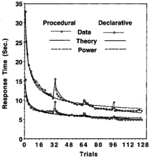
1122 ANDERSON, FINCHAM, AND DOUGLASS Figure 2 shows the data from the third experiment of J. R.

Anderson and Fincham (1994). That experiment extended over 4 days, and on each day participants had 32 blocks of practice either applying the rules or retrieving the declara-tive facts. In a block all items were tested once. Thus, there were 128 blocks total broken into four groups of 32 blocks, with each group separated by 1 day. To better expose the initial learning, for-each day we separately plotted Blocks 1, 2, 3; the average of Blocks 4 and 5; and men the average of successive sets of 3 blocks. Overall, there was a clear speed-up. However, at the beginning of each day there was a noticeable slowing from the previous day that largely disappeared after a few trials. Such initial slowing has been found in many studies (e.g., Adams, 1961; Postman, 1969; Schmidt, 1988), particularly in the motor skills literature, where there is a tradition of looking at learning effects at long delays. It is sometimes referred to as the warm-up decrement.

The model fit to the data in Figure 2 comes from a proposal of J. R. Anderson (1982) and J. R. Anderson and Schooler (1991) that the overall strength of a trace can be conceived as the sum of a number of individual strengthen-ings, each of which is decaying away as a power function. The strength function proposed by Anderson was the strength accumulation equation:

strength = t-d 7=1

where tj is the time that has passed since theyth occurrence of the item and the summation is over the n times the item has occurred. This equation adopts an interesting stance on the contrast between instance-based models and strength-based models of memory (e.g., Hintzman, 1976). It proposes that there is a single trace but that its aggregate strength is

Procedural Declarative Data

Theory

0 16 32 48 64 80 96 112 128 Trials

Figure 2. Latency results from the experiment of Anderson and Fincham (1994).

the summation of strengthenings from specific experiences, each of which is undergoing its own decay. J. R. Anderson, Bothell, Lebiere, and Matessa (1998) proposed that each item in the summation might be conceived of as reflecting new receptor sites at a synapse whose efficacies were decaying away as a function of time. However, it is also possible to interpret this equation as reflecting multiple traces, one for each occurrence, and the summation as reflecting accumulation of individuals' rates in a race model like that of Logan (1988). This equation also has an analogue to the sensory domain, where the perceived intensity of a stimulus can be thought of as the sum of a number of decaying perceptual traces (e.g., Cowan, 1987).

This strength accumulation equation serves as the basis for the strength mechanism in the ACT-R theory (J. R. Anderson, 1993; J. R. Anderson & Lebiere, 1998). Accord-ing to that theory latency to perform a task is an inverse function of this strength:

latency = A

Time (the tj) is measured in task blocks where each item is tested once in each block. Thus, a presentation of an item in Block 3 will have f, = 4 blocks by the time of Block 7. This function both predicts power-law retention effects and power-law practice effects. The power-law decay is directly built into the function. In addition, as J. R. Anderson (1982) showed, the summation approximately increases as a power function proportional to «( W ), where n is the number of

practices and d is the decay exponent in the strength accumulation equation.1

There are some complications in defining the items that go in the sum for application to the data in Figure 2:

1. On Day 1, there are three passes practicing the items before the experimental proper begins. This means that on Block 1, there are already three terms in the sum that we treated as 1,2, and 3 blocks old. There is only initial practice on Day 1, but these 3 extra practice trials are included in the calculations for the rest of the experiment.

2. Also not plotted in Figure 2 are 2 blocks of transfer trials at the end of each day's experimental Session 2. During these transfer trials each rule is tested once in each direction. These transfer trials should be added into the sum for later trials. These transfer trials occurred every day and were added into the sums for subsequent days.

3. There is the question of how to measure the passage of time (the tfi) across days. Suppose an item has age f,- = x blocks at the end of a day. What is its age m days later? The model we fit to the data assumes that tj = x + m*H blocks, where H is the number of blocks equivalent to a day's passage. Elliott and Anderson (1995) have found evidence that H is much less than would be estimated from clock time, suggesting that f, may measure something more like the

1 If the tj are evenly spaced, 2"= 1 tjd = ht~i1"=lj-d, where A?

is the spacing. The summation Z,J=1j~d can be approximated by calculating the integral $ j ~d dj = nl~dl(l - d).

number of interfering events. Similarly, McBride and Dosher (1997) have shown that forgetting rates tend to slow down dramatically after some period. Note that in this formula, we do not assume that time resumes its quicker pace once the next day's session begins. In a sense, the effects of earlier practices have been "consolidated" by the rest and continue to decay at their slow pace.

We estimated separate B parameters for the procedural and declarative tasks in Figure 2, and a single A, d, and H parameter. The A parameter represents the minimal response latency, and we set it to be equal for both conditions because the minimum response involved the same mouse clicks for both tasks. The B parameter reflects the difference in cognitive complexity of the tasks. The setting of the d and H parameters to be equal for both conditions reflects the simplifying assumption that the effects of delay will be the same for the procedural and declarative tasks. Minimizing sum squared deviation from predictions, the values esti-mated were B = 57.98 s for the procedural task, B = 20.71 s for the declarative task, A - 3.98 s, d = 0.61, and H = 9.59 blocks. The correspondence between the predictions and data is obviously good with an overall R2 of .986. (If we

allow separate A, d, and H parameters for the procedural and declarative tasks, the R2 only improves by .001.) The mean

deviation in the predictions of the procedural data is 0.58 s, whereas the standard deviation of the means2 in Figure 2 is

0.61 s. In the case of the declarative data, the mean deviation in the predictions is 0.47 s and the standard deviation of the means is 0.35 s. Thus, the quality of the fits is almost as good as could be expected given the noise in the data.3

One of the interesting aspects of this model is its account of the warm-up decrement. By the next day the most recent item is H = 9.59 blocks old, and the rest are even older. Thus, there are no recent delays contributing to the sum in the strength accumulation equation. At the end of the previous day, there were a number of recent delays that contribute dramatically to the sum. What happens over the first few trials of the new day is that some of these recent, large, but rapidly decaying increments get added to the overall strength. Once these have been added in again, the latency largely becomes a function of the total number of presentations. Thus, warm-up effects in retention reflect the introduction of the large but fast-decaying elements into the strength accumulation equation. This accounts for the obser-vations that retention improves dramatically given a re-fresher trial and that there are virtually no retention losses when one aggregates over many retention trials, washing out the warm-up decrement (Healy & Bourne, 1995).

As mentioned earlier, J. R. Anderson (1982) showed that this function is closely approximated by a power function with exponent 1 — d, where d is the decay rate. The smooth lines in Figure 2 show the best fitting power functions 3.38 + 23.59«-°41 fitted to the procedural data and 3.38 +

11.35n~041 fitted to the declarative data, where n is the

number of blocks (with the exponents of 0.41 and intercepts of 3.38 constrained to be equal). Except for the blips at the beginning of each day, these functions fit well. The R2

between these functions and the data is .966. Thus, the simple power function fits about 2% less of the variance than

the strength accumulation equation. Although this is not a large discrepancy, it involves the qualitatively critical data— long latencies at the beginning of the subsequent days. Note that the exponent estimate is almost exactly one minus the decay exponent (0.60) estimated for the strength accumula-tion equaaccumula-tion. This is what was predicted by J. R. Anderson (1982).

There are a number of significant aspects to this analysis based on the strength accumulation equation:

1. It integrates the effects of practice and retention into a single function that can predict trial-by-trial changes in latency.

2. It suggests that the effect of terminating the experimen-tal session is to slow down the decay clock. Items age 32 blocks over a session, but they age only another 9.59 blocks, between sessions. We call this the slowed-clock model, and at the end of this article we compare this with the proposal of a decreased forgetting rate. At the outset we should note that this may imply that clock time is not the right way to think of the critical variable. It might indicate that the critical variable is the number of intervening events and that there are fewer of these after the experimental session ends.

3. It suggests that the same memory dynamics apply to a relatively complex rule application as well as a simpler memory retrieval task. As suggested by J. R. Anderson (1982) and Rickard (1997), this may be because the components of a complex rule involve retrieval and the aggregate of these retrievals has dynamics that approximate the components.

This single strength accumulation equation offers a consid-erable integration to our understanding of retention and practice effects in memory. We report more data that will subject the strength accumulation equation to more demand-ing tests. We think that this research establishes the strength accumulation equation as the best characterization of the relationship between practice and retention.

In this article we describe four additional studies using this same paradigm to explore the results illustrated in Figure 2. Our basic manipulation in much of this research was to increase the retention intervals over which partici-pants had to remember material. This allowed both a better test of the underlying theory and the apparent observation that the psychological time increased only slowly after an experimental session. That is, by increasing the independent variable, time, we were enabling more powerful tests of its effect and its interaction with practice.

2 These standard deviations were calculated from the overall

Subject X Block interaction (where block refers to the points plotted in Figure 2). This was an attempt to get an estimate of noise in the data subtracting out participant effects. These were not totally satisfactory estimates of noise in condition means; the noise was probably higher in our estimates of the initial points because they had longer means and because they were based on single trials. Nonetheless, these standard deviation estimates provided us with some estimates of the accuracy of measurement that we could compare with accuracy in our predictions.

3 This fit and all others are available as Excel files from the

Published ACT-R Model link from the adaptive control of thought-rational (ACT-R) home page (http://act.psy.cmu.edu/).

1124 ANDERSON, FTNCHAM, AND DOUGLASS Experiment 1

In the first experiment we repeated the basic 4-day design of J. R. Anderson and Fincham (1994) but inserted either a week delay between Day 1 and Day 2 and then had Days 3 and 4 at 1-day delays (Condition 7-1-1), had 1-day delays for Days 1-3 and a week delay between Day 3 and Day 4 (Condition 1-1-7), or a month delay between Day 3 and Day 4 (Condition 1-1-30). The contrast between the first condi-tion and the other two allowed us to observe the effect of a longer delay on Day 2 performance. We should see an increased warm-up decrement when there is a week delay. The contrast between the first and second conditions also allowed us to study the effect of a week delay at different points in the practice curve. The warm-up decrement associated with a week delay should be less after 3 days of practice. Finally, the contrast between the second and third conditions allowed a further estimate of the impact of length of delay. In all cases, our concern was not just with qualitative effects but with the quality of fit with the predictions based on the strength accumulation equation given in the introduction.

Method

Participants. Thirty undergraduates (10 per condition) were recruited to participate in this 4-day experiment. Because of students not returning for later sessions, we were left with 8 participants in the 7-1-1 condition, 10 in the 1-1-7 condition, and 7 in the 1-1-30 condition. The first session lasted 2 hr, and the remaining 3 sessions lasted between 45 min and 1 hr. Participants were paid $4 per session. In addition, they received between $8 and $16 bonus pay that depended on performance.

Materials. Table 1 shows the abstract structure of the eight rules. Each participant saw different randomly generated examples that embodied these rules. All four possible relations (—2, — 1, + 1 , and +2) between the 2 hr and days occurred twice in the eight rules. Direction in Table 1 refers to whether the participant predicted the second time from the first (right) or the first from the second (left). Participants were randomly assigned to either Group 1 or Group 2.

Eight study examples were randomly generated, one for each rule. For each day's training session, 42 new examples were generated for testing each rule in the training and transfer phases. These training and transfer examples for each rule were different from one another and from the study example. However, there was no effort to avoid repetitions of examples across days.

Table 1

Abstract Structure of the Rules Used in Experiment 1

Pair A A B B C C D D )ay/hour + 1/+2 - 2 / - 1 -1/+1 +2/-2 -1/-2 +2/+1 + 1/-1 -2/+2 Direction practiced Group 1 Right Left Left Right Right Left Left Right Group 2 Left Right Right Left Left Right Right Left

Procedure. The same basic interface illustrated in Figure 1 was used in all phases of the experiment. The first day began with an initial exposure to the eight study examples followed by a three-pass dropout phase. During the initial exposure phase, participants were told to study each of the eight examples and copy them from the top row to the bottom row. This gave them the opportunity to memorize the examples and to familiarize them-selves wife fee interface before beginning fee dropout learning phase. In fee dropout phase, they were shown just fee sport name and had to reproduce the 2 days and 2 hr by means of mouse clicks. In each pass of fee dropout phase, they were tested repeatedly over fee items until they had correctly recalled fee times for each sport name. As soon as they recalled fee times for a name, it was dropped out of fee pass. The pass stopped when there were no more items. They were then tested on all fee items anew for another pass.

The dropout phase was followed by fee training phase in which participants would see just fee first day and hour and have to predict fee second or vice versa. However, they were required to click both fee day and hour for both fee first and fee second time, wife one pair being a copy and fee other pair being a prediction. If participants made an error, they were shown fee correct answer. The training phase for a day involved 40 blocks in which each rule was tested once.

The training phase was followed each day by a transfer phase in which each rule was tested once in both directions. This had been of interest in previous studies, in which we were looking at fee reversibility of fee rule knowledge. We do not analyze these transfer trials, but, as in fee fits to Figure 2, we counted them as 2 additional study blocks on feat day for purposes of applying fee strength accumulation equation on later days. Including these 2 extra blocks mattered little to fee predictions, but we kept them in fee equation for purposes of correctly representing fee participants' experience.

Results and Discussion

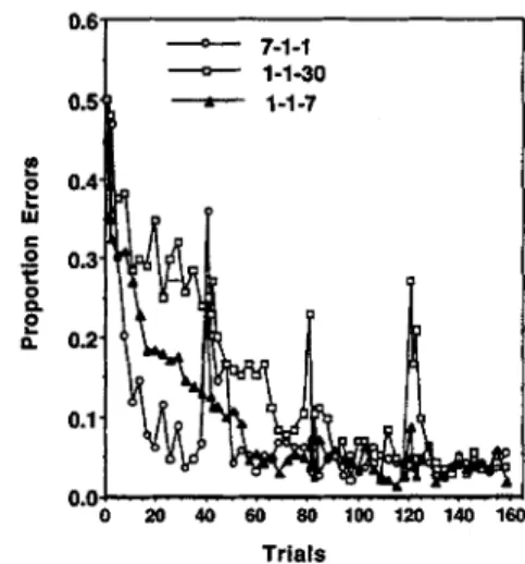
Figures 3 and 4 show error rate and latency4 as a function

of training blocks of practice. Again, we have separately plotted performance on the first 3 blocks of each day. After this, successive groups of 3 blocks have been collapsed together as a point except for the last 4 (37^40), which are plotted as a single point. In the case of aggregated blocks the data are plotted as a function of their average block number. There appear to be substantial differences in the perfor-mance of groups on the first day, where all participants were treated identically, but these differences among groups were not significant, F(2, 22) = 1.66, MSE = 500, for latency; F(2, 22) = 1.27, MSE = 0.991, for error rate. This reflects a phenomenon that we found throughout these experiments: There were large individual differences that could result in nonsignificant differences among the groups. However, the trends across blocks were stable within participants. Thus,

4 Trial latency is calculated as follows. The mouse cursor

position begins at fee location of fee OK button in fee middle of fee display. An internal starting time stamp is recorded at stimulus presentation time (fee maximum lag between time-stamp recording and screen refresh is approximately 17 ms). The participant must use fee mouse to click fee OK button at fee end of fee trial, at which point fee ending time stamp is recorded (fee maximum lag between mouse click and time-stamp recording is approximately 50 ms). Trial latency, in milliseconds, is gotten by subtracting fee starting time stamp from fee ending time stamp.

o

r

o

0 20 40 60 80 100 120 140 160 Trials

Figure 3. Proportion of errors in Experiment 1 as a function of block for the various delay conditions.

we had relatively powerful tests when examining within-groups effects using Subject X Block interactions for error terms.

With respect to the effects of retention interval, we conducted analyses of the transitions between Days 1 and 2 and between Days 3 and 4, comparing the mean perform-ance on the last 10 blocks of the prior day with the mean performance on the first 3 blocks of the subsequent day. The decrease in performance from the end of Day 1 to the beginning of Day 2 was significant for both measures, F(l, 22) = 4.74, MSE = 0.033,/? < .05, for error rate; F ( l , 22) = 30.76, MSE = 17.41, p < .001, for latency. There was a significant interaction between day and condition for error rate, F(2, 22) = 5.38, MSE = 0.033, p < .05, but not for latency, F(2, 22) = 1.15, MSE = 17.41. We expected that participants would show more of a loss over the 1-week retention interval. A contrast testing the error data for this was highly significant, *(22) = 3.28, p < .001. With

20 40 60 80 100 120 140 160

Blocks

Figure 4. Mean latency in Experiment 1 as a function of block for the various delay conditions.

respect to the transition between Day 3 and Day 4, the decrease in performance across days was significant for both measures, F ( l , 22) = 8.56, MSE = .016, p < .01, for error rate; F(l, 22) = 37.70, MSE = 3.12, p < .001, for latency. There was a significant interaction between day and condi-tion for both measures, F(2, 22) = 4.53, MSE = 0.016, p < .05, for error rate; F(2, 22) = 9.03, MSE = 3.12, p < .005, for latency. We expected that participants would show more of a loss over the 1-month retention interval than the 1-week interval. Contrasts testing for this were highly significant, r(22) = 2.42, p < .01, for error rate; f(22) = 3.68,/? < .001, for latency. The other expectation was that the loss would be greater over the week retention interval than the 1-day retention interval, but although the effects were in this direction, neither contrast testing this was significant, ?(22) = 0.43 for error rate; t(22) = 0.44 for latency.

We also compared participants' performance at the begin-ning of Day 4 (first 3 blocks) with their performance at the end of Day 4 (last 10 blocks). At the beginning there were significant effects of condition, F(2, 22) = 4.79, MSE = 0.041, p < .05, for error rate; F(2,22) = 15.64, MSE = 9.74, p < .001, for latency. At the beginning participants with the 1-month delay were worse than the other conditions, f(22) = 3.34, p < .001, for error rate; t(22) = 5.49, p < .001, for latency. On the other hand, by the end of the day there were no significant differences left among conditions, F(2,22) = 0.10, MSE = 0.003, for error rate; F(2, 22) = 2.29, MSE = 7.09, p < .1, for latency. The latency effect was marginal, and a contrast between the 1-month retention condition and the average of the other two conditions was significant, f(22) = 2.12, p < .05. Therefore, perhaps some residual difference remains by the end of Day 4.

Although not all the effects were significant, the general practice and retention effects are consistent with the results from J. R. Anderson and Fincham (1994), and we saw evidence for increasing beginning-of-day losses with increas-ing delays. However, significantly, these retention effects were largely eliminated at the end of one day's practice. In this article, we apply the strength accumulation equation only to predicting the latency results. Although the error data were noisier (and the equation did not directly apply), they were generally in the same direction as the latency data. There was a strong correlation between the errors and latencies in the experiment (r = .81).

We fit the same model to the latency data as described in the introduction for J. R. Anderson and Fincham (1994). As before, we used one A intercept parameter, one d exponent, and one H for the number of intervening blocks between days, but, to deal with the differences in the three groups of participants, we estimated separate B scale parameters. These parameters were d = .52, A = 3.54 s, H = 7.02 blocks,5 = 91.49 sfor the 1-1-30 condition, B = 61.70 sfor the 1-1-7 condition, and B = 71.92 s for the 7-1-1 condition. These parameters are similar to the parameters estimated for J. R. Anderson and Fincham's (1994) procedural condition. The R2 between theory and data was again a high .974. The

standard deviation of the predictions was 1.01 s, which was good given that the standard error of means (estimated from

1126 ANDERSON, FINCHAM, AND DOUGLASS the Subject X Block X Condition interaction) was 1.12 s.

Thus, it appears that the strength accumulation equation was capturing the same trends over a much larger manipulation of the retention intervals.

The model claims that the latency is composed of a fixed intercept (the A parameter—in this case 3.54 s) and a decreasing processing latency that is scaled by these B parameters. On the first block, the strength accumulation equation predicts that strength is I"0-52 + 2~0-52 + 3~0-52 =

2.26 (because of the three practices in the initial dropout learning phase) and by the end of the experiment strength is 19.33. Thus, the strength increases almost by a factor of 10 over the course of the experiment. This corresponds to the latencies dropping from about 35 s to 7 s over the course of the experiment. When the intercept of 3.5 s is subtracted, the latencies almost drop by a factor of 10.

The model was fit to the data in Figure 4, where each data point represents an average over participants, and many data points are averaged over multiple blocks for purposes of presentation. In the Appendix we briefly describe the results of fitting individual blocks for this experiment and the others in this article. The underlying quality of fit and the conclu-sions do not change.

Even using the aggregation in Figure 4, it was hard to determine critical data points and how well they were fit by the model. Not all of the numbers were equally critical to a test of the model. The most critical numbers were those that defined the transition between days. Therefore, we provide in Table 2 an analysis of performance on the last 10 blocks of a day and the first 3 blocks of the next day for the transitions between Days 1 and 2, 2 and 3, and 3 and 4. We also conducted a separate analysis of variance (ANOVA) to obtain more appropriate estimates of the noise in these means from the Subject X Condition interaction for those conditions. The standard error of the predictions was 1.05 s. This compares well with the 1.15-s SEM from the ANOVA. We need to emphasize that the model fit is to all the data in Figure 4. If we were to estimate the parameters just for the data in Table 2, we would reduce the mean error in prediction to 0.73. The serious point of discrepancy is at the beginning of Day 3 in the 1-1-30 condition, where

partici-pants took 12.33 s, but the model predicted only 9.25 s. This discrepancy can be seen in Figure 4, where the model underpredicts participant latencies in the 1-1-30 condition throughout Days 2 and 3. Probably more critical than whether we can predict the absolute latencies is whether we can predict the qualitative pattern in the warm-up decre-ments. These are somewhat independent of mean latency. The correlation between the predicted and observed warm-up decrements was .75. With respect to the warm-up decre-ments, the most systematic deviation was that the model underpredicted its size in the transition between Day 1 and Day 2 (the mean observed decrement was 3.13 s, and the mean predicted decrement was 1.77 s).

Experiment 2

Generally, the results of the previous experiment were consistent with the predictions of the strength accumulation model. However, it would be useful to get additional converging data. In addition, the high error rates and large differences between groups (apparently attributable to indi-vidual differences) make the conclusions less than totally satisfactory. Both of these problems may be due to the relatively difficult rule application task. Therefore, we decided to use a task in which participants only had to retrieve the instances. This corresponds to the declarative task in Figure 2 from J. R. Anderson and Fincham (1994). This will also extend the generality of our analysis by looking at a different task. In this experiment we used the same three delay groups as the first experiment but intro-duced a fourth group that practiced the items on 4 successive days. We refer to this as the 1-1-1 condition.

The experiment was also done to test whether the retention effects would be different for a procedural, rule-based task than for a declarative, retrieval-rule-based task. When we collected the data from Experiment 1, we were impressed with how quickly participants returned to near Day 3 levels after the 1-month retention interval in the 1-1-30 condition. We wondered whether such striking retention might be a fac-tor that separated a procedural task from a declarative task.

Table 2

Data (in Seconds) and Predictions for the Day-to-Day Transitions in Experiment 1 Condition Effect Day 1 end Day 2 start Warm-up decrement Day 2 end Day 3 start Warm-up decrement Day 3 end Day 4 start Warm-up decrement Data 11.20 15.30 4.10 7.53 7.53 0.00 6.07 6.70 0.63 7-1-1 Prediction 10.84 14.25 3.58 8.35 8.62 0.36 6.75 6.95 0.20 Data 9.13 11.40 2.27 8.10 7.43 -0.67 6.23 7.10 0.87 1-1-7 Prediction 9.80 10.50 0.70 7.15 7.39 0.25 6.09 7.13 1.04 Data 12.40 15.43 3.03 10.03 12.33 2.30 8.07 11.83 3.76 1-1-30 Prediction 12.83 13.86 1.03 8.89 9.25 0.36 7.32 12.08 4.77

Method

The procedure was identical to that used in previous experiment, except that all trials involved presenting the days and sport from the study example (or the hours and sport) and participants had to reproduce both the days and hours from the example. Thus, they were recalling either the days or the hours given the other. There were 11 participants in the 1-1-1 condition, 9 participants in 7-1-1 condition, 11 participants in the 1-1-7 condition, and 8 participants in the 1-1-30 condition.

Results and Discussion

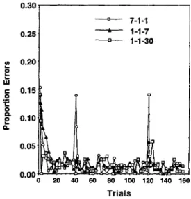
Figures 5 and 6 show error rates and latencies as a function of serial position. We have omitted the data from the 1-1-1 condition because it would have resulted in graphs that were too cluttered. Again, we have plotted performance on the first 3 blocks of each day. There were small differences among the groups, but statistical tests revealed no significant differences, F(3, 35) = 0.92, MSE = 103.44, for latency; F(3, 35) = 0.02, MSE = .014, for error rate. With respect to the effects of retention interval, we con-ducted analyses of the transitions between Sessions 1 and 2 and between Sessions 3 and 4 comparing the mean perfor-mance on the last 10 blocks of the prior session with the mean performance on the first 3 blocks of the subsequent session. With respect to the transition between Session 1 and Session 2, the decrease in performance from the end of one day to the start of the next was significant for latency, F(l, 35) = 21.99, MSE = 4.85, p < .001, but not for error rate, F ( l , 35) = 1.50, MSE = 0.009, although it was in the expected direction. There was a significant interaction between session and condition for latency, F(3, 35) = 3.09, MSE = 4.85,p < .05, but not for error rate, F(3,35) = 1.73, MSE = 0.009. We expected that participants would show more of a loss in the condition that had a 1-week retention interval than the other conditions. A contrast testing for this was significant for both dependent measures, r(35) = 2.27,

0.30

0.00

20 40 60 80 100 120 140 160

Trials

Figure 5. Proportion of errors in Experiment 2 as a function of block for the various delay conditions.

0 20 40 60 80 100 120 140 160

Trials

Figure 6. Mean latency in Experiment 2 as a function of block for the various delay conditions.

p < .05, for error rate; f(35) = 2.61, p < .01, for latency. With respect to the transition between Session 3 and Session 4, the decrease in performance across session was significant forrxrthmeasures,F(l,35) = 9.14,MSE= 0.003,p< .005, for error rate; F ( l , 35) = 5.29, MSE = 3.61, p < .05, for latency. The interaction between session and condition was not significant for either measure, F(3, 35) = 1.67, MSE = 0.003, for error rate; F(3, 35) = 2.84, MSE = 3.61, p < .10, for latency. We expected that participants would show more of a loss over the 1-month and 1-week retention intervals than the 1-day intervals. Contrasts testing for this were significant (two long retention intervals minus two short retention intervals), f(35) = 2.04, p < .05, for error rate; f(35) = 2.61, p< .01, for latency. The other expectation was that the loss would be greater over a month than a week, but, although the effects were in that direction, neither contrast testing this was significant, f(35) = 1.13 for error rate; f(35) = 1.50 for latency.

We also compared participants' performance at the begin-ning of the Session 4 (first 3 blocks) with their performance at the end of Session 4. At the beginning, there were effects of condition, F(3, 35) = 2.25, MSE = 0.0062, p < .10, for error rate; F(3, 35) = 3.27, MSE = 7.91, p < .05, for latency, and participants with the 1-month delay were worse than in the other conditions, f(35) = 2.30, p < .01, for error rates; f(35) = 3.09, p < .005, for latency. On the other hand, by the end of the session, there were no significant differ-ences left among conditions, F(3, 35) = 1.79, MSE = 0.0007, for error rate; F(3, 35) = 1.16, MSE = 7.09, for latency.

In summary, although not all the effects were significant, the results are generally consistent with the first experiment and with expectations. This occurred despite the fact that we used a task with much lower error rates and much faster latencies. There was a substantial correlation between the error rate and latencies in this experiment (r = .71). Again,

1128 ANDERSON, FBSfCHAM, AND DOUGLASS we used the strength accumulation equation to fit the latency

data.

We fit the same model to the latency data as described for Experiment 1. Again, to deal with the differences in the participants in the four groups, we estimated separate B scale parameters but used one A intercept parameter, one d exponent, and one H for the number of intervening blocks between days. These parameters were d = .76, A = 3.85 s, H = 4.55 blocks, B = 18.35 s for the 1-1-30 condition, B = 16.79 s for the 1-1-7 condition, B = 19.20 s for the 7-1-1 condition, and B = 22.59 s for the 1-1-1 condition. The R2

between theory and data was .935. The standard deviation of the predictions was 0.46 s, which was good given that the standard error of means (estimated from the Block X Condition X Subject interaction) was 0.43 s. The d parameter was larger than in previous fits and the H parameter smaller. However, there was a trade-off between these two parameters because both affected the rate of forgetting. If we constrain d to be .6 (the value in the fit to Anderson & Fincham's, 1994, Figure 2), the new estimate of H is 10.69 (close to the 9.23 estimated for Figure 2). The R2

for this more constrained model decreases only to .927, as compared with .935 for the unconstrained model.

In a manner similar to Table 2, Table 3 shows the critical transition data for Experiment 2. The mean deviation was 0.42 s, compared with a standard error of 0.36 s from the Condition X Subject interaction for these cells. Again, we emphasize that this was a fit constrained by the total data in Figure 6. If we were just to fit the numbers in Table 3, our mean error of prediction would be 0.23. If we look at the correspondence between the predicted and observed warm-up decrements, the correlation is .78. As in Table 2, there was some tendency for the model to underpredict the warm-up decrement from Day 1 to Day 2 (mean observed = 1.35 s, mean predicted = 0.92 s).

Experiment 3

The results from the first two experiments are generally consistent with the model that we have been proposing. However, a still more strenuous test of the theory would involve even longer retention intervals. Therefore, we

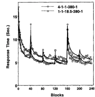
decided to try to retrieve as many participants as we could from the second experiment at a much longer retention interval, which varied from 11 to 14 months. We were able to get 11 of the original participants back, 3 from each condition except the 7-1-1 condition, from which we got only 2 participants. We decided to aggregate the three 1-1-1 participants and the two 7-1-1 participants into a group that did not have an elongated retention interval after Day 3 and the three 1-1-7 participants and the three 1-1-30 participants into another group that did. The average retention interval to the 5th day was 380 days. To further examine relearning, we followed the 5th day with a 6th day of training. Thus, we refer to the first group as 4-1-1-380-1 and the second group as 1-1-18.5-380-1 to reflect the average retention intervals. The procedures on the 5th and 6th days were identical to what they had been on the first 4 days.

Figures 7 and 8 show errors and latency as a function of serial position. Participants showed a substantial perfor-mance decrement on Session 5 after the long retention interval, but their performance on Session 6 was almost identical to the performance on Session 4 (mean latencies of 5.61, 7.04, and 5.52 s for Sessions 4, 5, and 6, respectively, and mean error rates of 2.1%, 14.2%, and 1.7%, respec-tively). Although participants fully recovered in the sixth session, their deficit in Session 5 remained throughout the session. Although it was most dramatic for the first few blocks, it was not just confined to these. Thus, with sufficiently long delay the warm-up decrement was much more extensive. Kolers (1976) also found more permanent decrements when he studied reading of inverted text a year after original training.

We fit the same model to the latency data as for the earlier experiments. For the average of the 1-1-1 and 7-1-1 conditions, we used an average delay of 4 days between the first pair of sessions. Thus, the retention intervals were 4, 1, 1, 380, and 1 day. For the average of the 1-1-7 and 1-1-30 conditions, we used an average delay of 18.5 days between the third and fourth sessions. Thus, the retention intervals were 1,1, 18.5, 380, and 1 day. The parameters were d = .38,A = 4.13 s,H = 74.1 blocks for all the days, B = 31.81 s for the average of the 1-1-1 and 7-1-1 conditions, and B =

Table 3

Data (in Seconds) and Predictions for the Day-to-Day Transitions in Experiment 2 Condition Effect Day 1 end Day 2 start Warm-up decrement Day 2 end Day 3 start Warm-up decrement Day 3 end Day 4 start Warm-up decrement Data 7.37 8.97 1.60 5.97 6.73 0.77 5.70 5.83 0.13 1-1-1 Prediction 7.65 8.36 0.71 6.14 6.40 0.26 5.50 5.83 0.16 Data 7.13 9.87 2.73 5.93 5.83 -0.10 5.67 5.37 -0.30 7-1-1 Prediction 7.08 8.93 1.85 6.07 6.31 0.24 5.37 5.51 0.14 Data 6.43 6.83 0.40 5.60 6.00 0.40 5.07 5.77 0.70 1-1-7 Prediction 6.67 7.20 0.53 5.55 5.75 0.20 5.08 5.67 0.59 Data 7.53 8.30 0.77 5.87 6.53 0.67 5.87 7.67 1.80 1-1-30 Prediction 6.93 7.51 0.58 5.71 5.92 0.21 5.19 8.02 2.83

0.8: 0.7 0.6 0.5 4-1-1-380-1 1-1-18.5-380-1 80 120 160 200 Blocks 240

Figure 7. Proportion of errors in Experiment 3 as a function of block for the various delay conditions.

20.71 s for the average of the 1-1-7 and 1-1-30 conditions. The R2 between theory and data was .897. The standard

deviation of the predictions was 0.63 s, which was good given that the standard error of means (estimated from the Block X Condition X Subject interaction) was 0.60 s. The values of d and H were deviant from prior fits. However, if we constrain d to .50, the lowest value it had in prior experiments, the best fitting parameters become H = 13.40 blocks, A = 4.15 s, and Bs = 28.69 and 18.65 s. These parameters are more consistent with previous parameters, and the R2 went down to only .885 and standard deviation up

to 0.66 s. Again, the model was not very sensitive to the particular combination of the H and d parameters. This

0 40 80 120 160 200 240

Table 4

Data (in Seconds) and Predictions for the Day-to-Day Transitions in Experiment 3 Effect Day 1 end Day 2 start Warm-up decrement Day 2 end Day 3 start Warm-up decrement Day 3 end Day 4 start Warm-up decrement Day 4 end Day 5 start Warm-up decrement Day 5 end Day 6 start Warm-up decrement Condition 4-1-1-380-1 Data 7.40 10.39 2.99 6.27 7.07 0.80 5.97 6.03 0.07 5.53 11.11 5.60 6.03 5.87 -0.17 Prediction 6.93 8.47 1.54 6.02 6.28 0.25 5.45 5.61 0.17 5.17 11.73 6.56 6.44 6.75 0.31 1-1-18 Data 6.43 6.73 0.30 5.17 5.40 0.23 4.80 6.23 1.43 5.00 9.60 4.60 5.60 5.37 -0.23 .5-380-1 Prediction 5.95 6.37 0.41 5.24 5.41 0.25 4.94 5.96 1.02 5.13 9.15 4.02 5.65 5.86 0.21

Figure 8. Mean latency in Experiment 3 as a function of block for the various delay conditions.

version of the model with d constrained to .50 is the one we refer to in the General Discussion section.

Table 4 shows the critical transition data from Experiment 3 in a manner similar to Tables 2 and 3. The model generally did a good job of capturing the data with an overall correlation of .941. The mean deviation was 0.61 s, which compares with the standard error of 0.50 s from the Condition X Subject interaction for these cells. Again, we emphasize that the model was fit to all the data, and the mean deviation would be much reduced (only 0.37 s) if we confined ourselves to the data in Table 4. The greatest discrepancy reflects the same problem that we noted for Table 3. This is between the times for the beginning of Day 2 in the 4-1-1-380-1 condition, where the model underpredicts the degree of loss over this 7-day period. Again, perhaps the most critical test is the correlation between the predicted and observed warm-up decrements. This correlation was .95. Strong support for the theory is the success at predicting the size of the warm-up decrements at 1-year delays.

Experiment 4

The current model offers an interesting explanation of some aspects of the spacing effect (e.g., Bahrick, 1979). The slowed-clock model hypothesizes that effective time passes more slowly after an experimental session. If a day interval is worth H blocks of trials, then if one is going to have more than 2H blocks it is better to split them over 2 days. As an illustration, suppose one is going to administer AH blocks of practice and contrast massing all AH blocks on one day with splitting them so that 2H blocks on one day are followed by another 2H blocks on the next day. Consider performance after the AH blocks. The cumulative impact of the last 2H blocks will be identical in both conditions because they will have occurred at delays varying from 1 to 2H blocks on that day. In the massed conditions the first 2H blocks will have

1130 ANDERSON, FINCHAM, AND DOUGLASS delays from 2H + 1 to AH. In the split condition, the delay

will be H (for the day delay) plus however many blocks followed that practice on the first day. Thus, the delays for the first 2H blocks will be from H + 1 to 3H, which is H less than in the massed condition. Basically, the argument is that if one masses too many trials together, one will create a situation in which the extra trials are doing almost as much harm as good by accelerating forgetting. Inserting a day's rest slows down the forgetting processes. We would not want to suggest that this is all there is to the spacing effect, which is a complex phenomenon (e.g., see discussions in Crowder, 1976; Greene, 1989; Kahana & Greene, 1993), but it may be a contributing factor.

We decided to contrast participants practicing 24 blocks a day with participants practicing 48. Our estimates of H from previous experiments were all around 12, and so 48 would be about the AH from the previous paragraph. One of our interests was in how well participants would be doing after 48 blocks (after either 1 day or 2 days) and after 96 blocks (after either 2 days or 4 days). Both groups worked on the task for 4 days to be consistent with the design of the previous experiments and to give us additional data about the effects of practice and retention intervals. Like in Experiment 1 and unlike in Experiments 2 and 3, the test in this experiment used rule application rather than simple example recall.

This experiment involved a second manipulation that was motivated to investigate the nature of performance in the rule-application task. Because participants in past experi-ments started with examples and not rules, they would have to initially extract the rales by analogy. They should be at a deficit to participants who learned the rules directly because of this extra analogy step. We wanted to confirm that this was so and to determine whether the deficit would be maintained over the course of the experiment. Therefore, we had conditions that contrasted participants learning the rules directly with participants learning examples as in past experiments. Although we report the effects of the training procedures, our main interest in this article was in the manipulation of 24 versus 48 blocks per day.

Method

This experiment was like Experiment 1, with participants receiving 4 successive days of practice and getting either 24 or 48 blocks of practice per day. Each day was followed with a transfer test of two blocks. There was the other manipulation of how participants were trained. We contrasted four conditions:

Condition 1. Examples only: Studied eight examples as in previous experiments.

Condition 2. Rule only: Studied the eight rules behind the examples directly.

Condition 3. Example plus rule: Studied both examples and rules (i.e., a combination of Conditions 1 and 2).

Condition 4. No prior training: These participants would have to infer the rules from the feedback given during testing.

Except for Condition 4, all participants went through the same triple dropout procedure as used in the earlier experiments. In Condition 2 they had to produce the rules (e.g., +2 days, —1 hr), and in Condition 3 they had to produce both examples and rules.

We experimented with these four training conditions because we wanted to determine whether there would be any effect of having to extract the rules by analogy (i.e., Condition 1, which is the only condition used in prior research). Thus, there were eight groups of participants created by crossing number of trials per day (24 vs. 48) within training (four conditions). There were 5 participants as-signed to each group.

Results and Discussion

ANOVAs were conducted on latencies and errors in which the factors were training procedure (4 values), blocks-per-day (2 values), days (4 values), and block-within-day (10 values: 1,2,3,4-6,9-12,13-15,16-18,19-21, and 22-24). Note that in these ANOVAs, we were looking only at the first half of the blocks each day for participants receiving 48 blocks per day.

Because some participants in the no-prior-training condi-tion needed a few blocks before they got anything right, we aggregated latencies differently for purposes of this ANOVA. For each rule we counted blocks as trials on which a participant got the answer right. For instance, suppose a participant made errors on a rule on Blocks 1, 2, and 4 and was correct otherwise. In assigning blocks to this rule, Block 1 would actually be Block 3 (first correct), Block 2 would be Block 5, Block 3 would be Block 6, and so on. For latencies, the block-within-day factor was extended only to Block 18 so that all participants had latencies defined for all cells.

With respect to latency, all main effects were significant: training procedure, F(3, 96) = 5.18, MSE = 307.4,/? < .01; blocks per day, F ( l , 32) = 5.56, MSE = 307.4,/> < .05; day, F(3, 96) = 213.46, MSE = 50.62, p < .001; and block within day, F(7,224) = 82.82, MSE = 8.13,/? < .001. With respect to training procedure, the examples-only participants were slowest (15.31 s), as suspected, followed by rule only (12.35 s), followed by example plus rule (10.88 s), followed by no prior training (10.66 s). The difference between the examples-only and the other conditions was significant, t(96) = 3.55,p < .001, whereas the residual variance among the other three conditions was not, F(2,96) = 1.47. Some of the interactions of training procedures with days and blocks within days were significant, but this was because the absolute size of differences reduced with practice (but did not change direction). For instance, the examples-only group averaged 25.27 s on Day 1 and the others averaged 17.86 s. By Day 4 this was 10.05 s for the examples-only group and 7.69 for the other three. Thus, it appears that the examples-only group, unlike the other conditions, were slowed by having to go through an analogy process and this continued to the end of the experiment.

With respect to error rate, only the within-subjects main effects were significant, not the between-subjects factors: day, F(3, 96) = 36.08, MSE = 0.202, p < .001; and block within day, F(9, 288) = 52.93, MSE = 0.007, p < .001; training procedure, F(3, 32) = 0.68, MSE = 0.601; and blocks per day, F ( l , 32) = 0.01, MSE = 0.601. There were significant interactions of training condition both with trial, F(27, 288) = 5.59, MSE = 0.007, p < .001, and with trial and day, F(81, 864) = 3.93, MSE = 0.011, p < .001. These interactions reflect the poor initial performance of the

2 ui o ••E o a 2 a.

24 Blocks Per Day 48 Blocks Per Day

Table 5

Comparison of Transfer Performance After Comparable Practice Transfer Results: Latency and Error Rates

24 48 72 96 120 144 168 192

Blocks

Figure 9. Proportion of errors in Experiment 4 as a function of block for the various delay conditions.

participants with no prior training who did not get below 50% errors until after the sixth block. However, the accuracy difference between this condition and the others disappeared by the end of the 1st day. Both with respect to latency and accuracy, there were not significant sample or higher order interactions involving training condition and blocks per day (24 vs. 48). The latter factor was the manipulation of interest in this experiment. Because it did not interact with training procedures, we could safely collapse it over training proce-dures in the further analyses.

24 Blocks Per Day 48 Blocks Per Day

24 48 72 96 120 144 168 192

Blocks

Figure 10. Mean latency in Experiment 4 as a function of block for the various delay conditions.

Condition 24 Blocks a day Latency (s) % error 48 Blocks a day Latency (s) % error Average Latency (s) % error Test after 48 blocks 12.41 9.2 11.95 15.5 12.18 12.4 Test after 96 blocks 8.86 3.6 9.69 13.8 9.28 8.7 Average 10.63 6.4 10.82 14.7

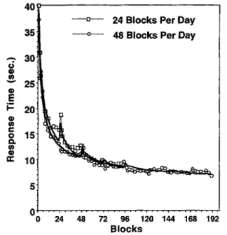
Figures 9 and 10 show error rate and latency as a function of blocks of practice collapsed over training condition.5

Because the 48-block participants practiced twice as much, their curves extend out twice as long. We have separately plotted the first 3 blocks of every 24 because this would be a new day for participants receiving 24 blocks a day. With respect to latency, participants appeared to be speeding up equally as a function of blocks. With respect to error rate, the participants appeared to be improving faster in the 24-blocks-per-day group. The best tests of a difference between the groups were the transfer tests that followed every 48 blocks. Table 5 shows the transfer results after 48 blocks and 96 blocks. There were highly significant effects of time of test (after 48 or 96 blocks), F ( l , 38) = 26.02, MSE = 16.11,p < .001, for latency; F ( l , 38) = 0.99, MSE = 0.0526, for error rate. There was a tendency in this experiment for better performance in the 24-blocks-per-day condition, as pre-dicted. However, the effects of number of blocks per day were not significant for either measure, F(l, 38) = 0.03, MSE = 47.07, for latency; F(l, 38) = 2.57, MSE = 0.1057, for error rate. The interactions between the factors were also not significant.

Still, the data displayed in Figure 9 manipulated the amount of practice while holding time constant and so offered a new combination of delay and practice and was a good challenge to our model. The best fitting parameters were d=.44,A = 5.48 s, H = 14.00 blocks, and B = 68.25 s for the 48-blocks-per-day condition, and B = 77.32 s for the 24-blocks-per-day condition. The R1 between theory and

data was .983. The standard deviation of the predictions was 0.75 s, which was good given that the standard error of means (estimated from the Block X Condition X Subject interaction) was 0.72 s.

5 Unlike in the analysis of variance reported, the mean for block

n came from just the correct rule applications in the original nth block and we did not move the correct latencies forward so that all rules had a latency for that block. If a participant in the no-prior-training condition did not have any correct responses for a block, the mean latency for that participant was simply omitted in calculating the averages in Figure 10.

1132 ANDERSON, FINCHAM, AND DOUGLASS

Table 6

Data (in Seconds) and Predictions for the Day-to-Day Transitions in Experiment 4 Effect Day 1 end Day 2 start Warm-up decrement Day 2 end Day 3 start Warm-up decrement Day 3 end Day 4 start Warm-up decrement Condition 24 trials Data 15.98 16.34 0.36 12.18 10.98 -1.19 9.55 9.28 -0.27 Prediction 14.55 15.73 1.19 11.03 11.47 0.44 9.49 9.84 0.35 48 trials Data 10.82 12.03 1.20 8.98 8.23 -0.76 8.00 7.47 -0.53 Prediction 10.56 11.35 0.79 8.34 8.72 0.38 7.53 7.76 0.24

Table 6 shows the critical transition data from Experiment 3. For these data the average for end of day was obtained from the last three means for that day in Figure 10. The mean deviation of the predictions was 0.69 s, which compared with a standard error of 0.51 s from the Condition X Subject interaction for these cells. Again, this reflects the constraints of fitting the data as a whole: We can reduce the mean deviation in prediction to 0.30 if we fit only the data in Table 6. The greatest discrepancy is that the model underpredicted latency at the end of Day 1 in the 24-block-a-day condition. This was part of a more general trend, which can be seen in Figure 10, of underpredicting the data in the period from the end of Day 1 to the end of Day 2 in that condition. The overall correlation between the predicted and observed warm-up discrepancies was .66, which was lower than in previous experiments. This partly reflects the fact that there was no multiday delays in this experiment that produced large warm-up decrements. There was a peculiar tendency for the warm-up decrements to be negative in later days in this experiment. However, basically, the theory and data agree that the warm-up decrement was negligible after the 1st day. Unlike previous experiments, the model did not underpredict the warm-up decrement from Day 1 to Day 2 (observed = 0.78 s, predicted = 0.99 s). Therefore, this is probably not a systematic problem with the model.

General Discussion

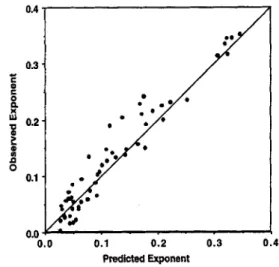
As can be seen by visual inspection of Figures 2, 4, 6, 8, and 10, the strength accumulation equation did a good job of accounting for the qualitative nature of the latency patterns as a function of amount of practice and delay. Tables 2, 3,4, and 6 are an attempt to focus in one important aspect of this qualitative pattern, which was the warm-up decrement, and the theory generally did well in capturing that. The warm-up decrement measured the loss from one day to the next. One can also try to capture the rate of learning within days, and Figure 11 is an attempt to summarize our success in fitting that qualitative aspect of these data. As an inspection of Figures 2, 4, 6, 8, and 10 reveals, the within-days learning functions were very much a function of amount of practice

and delay. Within-days learning tended to disappear as participants had massed more days of practice. To obtain an estimate of the rate of learning within days, we fit simple power functions of the form T = AP~C to the latency data

and predictions for each day and condition. In this equation A and c are estimated parameters and P is the number of trials of practice within each day. This was just a simple descriptive effort to estimate exponents c, which would serve to reflect rate of learning for that day. Altogether, we obtained 56 pairs of observed and predicted exponents (8 from Figure 2, 12 from Figure 4, 16 from Figure 6, 8 from Figure 8, and 8 from Figure 10). (An Excel file providing the estimation is available with the other files for this article; see Footnote 3.) Figure 11 displays the observed exponents as a function of the predicted exponents. As is apparent, the overall correlation was high (r = .962). This indicates that the strength accumulation equation did capture the within-days differences in learning rates.

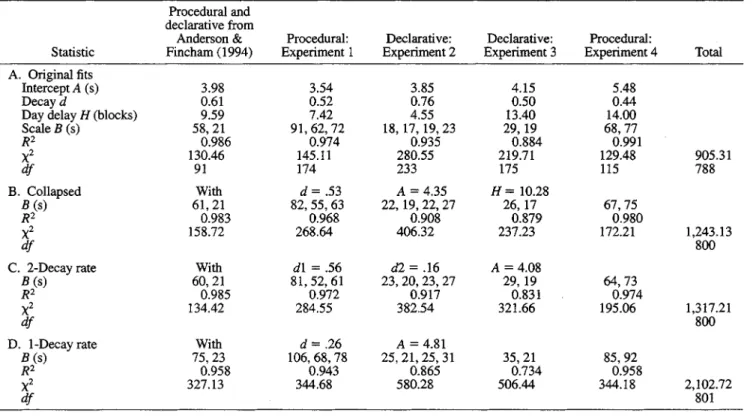
We now turn from summarizing our ability to predict the qualitative patterns to discussing measures of quantitative fits and alternative models. Table 7a shows the parameters estimated for each of the experiments and the goodness of fit. The A, d, and H parameters were relatively consistent across experiments. For each condition of each experiment, we estimated a different B parameter. The B parameters were much larger for the procedural tasks than the declarative tasks, reflecting their greater difficulty. In experiments that involved a procedural task, the B parameters ranged from 58 to 91 s, whereas the declarative tasks ranged from 18 to 29 s. The differences in B were sometimes large even within an experiment, reflecting the large individual differences. The B parameters essentially served to compensate for individual differences and served much like subtracting out subject variance in an ANOVA.

Another way of investigating the success of the model was to compare the size of the deviations with the standard error of the mean for each condition (calculated by the Subject X Block interaction for that condition). The summed

o.o 0.1 0.2 0.3

Predicted Exponent

Figure 11. Relationship between predicted and observed days learning exponents. The data plotted are for all the within-days learning curves in Figures 2,4,6, 8, and 10.

deviations divided by the squared mean error is a chi-square statistic with a number of degrees of freedom being equal to the number of observations minus the number of parameters. Table 7 shows these square statistics. The total chi-square statistic over the experiments was 905.31. The total degrees of freedom were 816 (total number of observations) - 2 8 (parameters) = 788. With these large numbers of degrees of freedom, the chi-square was distributed normally with a variance being equal to twice the degrees of freedom. Thus, the chi-square was distributed with a mean of 788 and a standard deviation of 39.7. The observed chi-square was 2.95 SDs away and was significant by standard measures. Therefore, although the overall fits were good, we cannot claim to have captured everything in the data. However, it is an unrealistic expectation to fit every nuance in the data.

To provide a more constrained model, we tried to fit a single d, A, and H parameter, allowing for separate B parameters for each condition. This reduced the number of degrees of freedom by 12 and is reported in Table 3. The new chi-square value was 1,243.13, which was significantly different from the mean for a chi-square with 800 dfs and a standard deviation of 40. It was also more than 300 larger than the chi-square when we fit each experiment separately. Still, the R2 remained high. We view this as a better model

because of the reduction in degrees of freedom. We have observed in individual experiments that the parameter estimates (particularly d and H because they both affected the rate of forgetting) tended to trade off and that this combined fit provided much greater constraint on their estimation. For instance, we found the best estimates of d

varied from .38 (Experiment 3) to .76 (Experiment 2). If we constrain dto be .38 the chi-square jumps to 1,460, and if we constrain it to be .76 it jumps to 1,721. Thus, the combined experiments provided stronger constraints on the parameter estimates.

Two of the parameter values obtained in this constrained fit are interesting. First, note the estimate of H, which implies that each day of retention after the initial training is worth just more than 10 blocks of trials. Ten blocks of trials would have taken 10-15 min in the experiments. Thus, effective time has slowed down by a factor of more than 100. Second, the d parameter is estimated to be .529, which is close to the .50 value, which has been proposed in the ACT-R theory (Anderson & Lebiere, 1998), which uses the strength accumulation equation.

Table 7 also shows two other models for comparison. An obvious alternative to the slowed-clock model is to assume that the decay rate changes with time. According to this two-decay model, after the end of an experimental session a different decay parameter would become effective. Thus, the total strength of presentation at some time t2 (greater than its

age tx at the end of the experimental session) would be

strength = -dl

The best fitting version of this model is shown in Table 3. It has d\ estimated at 0.564, which is similar to the 0.534 for the other model, whereas the second slower decay rate dl is 0.159. This model fits somewhat worse overall with a total

Table 7

Summary of Various Models From the Experiments

Statistic A. Original fits Intercept A (s) Decay d

Day delay H (blocks) Scale B (s) R2 X2 df B. Collapsed B(s) R2 X2 df C. 2-Decayrate £(s) R2 X2 df D. 1-Decay rate B(s) R2 X2 df Procedural and declarative from Anderson & Fincham (1994) 3.98 0.61 9.59 58,21 0.986 130.46 91 With 61,21 0.983 158.72 With 60,21 0.985 134.42 With 75,23 0.958 327.13 Procedural: Experiment 1 3.54 0.52 7.42 91,62,72 0.974 145.11 174 d= .53 82, 55,63 0.968 268.64 dl = .56 81,52,61 0.972 284.55 rf=.26 106, 68,78 0.943 344.68 Declarative: Experiment 2 3.85 0.76 4.55 18,17,19, 23 0.935 280.55 233 A = 4.35 22,19, 22,27 0.908 406.32 <*2 = .16 23,20, 23, 27 0.917 382.54 A = 4.81 25,21,25,31 0.865 580.28 Declarative: Experiment 3 4.15 0.50 13.40 29,19 0.884 219.71 175 H = 10.28 26,17 0.879 237.23 A = 4.08 29,19 0.831 321.66 35,21 0.734 506.44 Procedural: Experiment 4 5.48 0.44 14.00 68,77 0.991 129.48 115 67,75 0.980 172.21 64,73 0.974 195.06 85,92 0.958 344.18 Total 905.31 788 1,243.13 800 1,317.21 800 2,102.72 801

1134 ANDERSON, FINCHAM, AND DOUGLASS chi-square of 1,317.21. It is not much different from the

slowed-clock model except for Experiment 3, in which we used delays of more than a year. Here, the R2 is reduced from

.879 to .831, and the chi-square increases by more than 80. The final model (in Table 3) we tested was one with a single decay and no slowing of the clock. This model has 801 dfs, which is one more than the models in Table 3. The d parameter for this model estimates to be .259 and the A parameter is 4.80. This model fits much worse, with a total chi-square of 2,102.72. Thus, we are clearly gaining some-thing by estimating a slowing of the decay process by either the slowed-clock model or the two-decay-rate model.

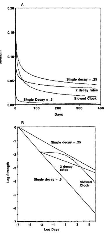
Figure 12 provides an analysis of the various models in Table 7. It shows what happens to the strength of a trace introduced on the first block of a 40-block experiment under various decay models. Figure 12A shows the decay in normal scale, and Figure 12B shows the decay in log-log scale. The log-log scale representation is more revealing. The two straight lines reflect what happens with simple decay rates of 0.5 (approximately the decay rate estimated in Table 3 and the faster decay rate in Table 3) and 0.25 (approximately the rate estimated in Table 3). Three lines diverge from the 0.5 decay line at the point corresponding to the end of the day's experiment. The steep line (for the single-decay model) reflects what would happen if decay continued at 0.5 and the shallow straight line (for the two-decay model) reflects the slower decay of 0.16 esti-mated in Table 3. The curved line (for the slowed-clock model) reflects what happens in Table 3 when the clock slows. Initially, the decay for the slowed-clock model slows dramatically but eventually crosses over the two-decay model and becomes parallel to the 0.5 decay slope. The differences between the slowed-clock and two-decay models become large after a year, and this is why the slowed-clock model does better than the two-decay model in Experiment 3.

This research is consistent with a number of other reports that forgetting slows down with time even beyond the slowing that is predicted by a power function (e.g., McBride & Dosher, 1997; Wickelgren, 1972). The research presented in this article was not designed to carefully identify the nature of this slowing process. Although the slowed-clock model gave the better fits, it must be remembered that this model may point only in the direction of an exact character-ization of the forgetting process. For instance, it may not be true clock time that is relevant. It is possible that the critical variable is the number of intervening similar events and that the slowing of the clock simply reflects their decreased occurrence after the experimental session, perhaps reflecting a change in context. Also, although we have simply charac-terized the change in the clock speed as a discrete shift occurring at the end of the experimental session, it is possible that there is some more gradual slowing.

Another result from this research, which is consistent with other reports, is that the same forgetting process seems to characterize both retrieval (we called this a declarative task) and rule-based processing (we called this a procedural task). Rubin and Wenzel (1996) found similar retention functions for a wide variety of material. McBride and Dosher (1997)

i

_

Figure 12. Comparison of the strength decay curves for the various models in Table 3. A: Normal plot. B: Log-log plot.

found similar functions for implicit and explicit memory. Thus, it seems that the forgetting functions of memory have strong similarities across tasks.

Although the results of this research confirm and extend other research on the forgetting function, its more novel contribution is integrating these retention effects with