Efficient Tests of Stock Return Predictability

NBER WORKING PAPER SERIES

EFFICIENT TESTS OF STOCK RETURN PREDICTABILITY John Y. Campbell

Motohiro Yogo Working Paper 10026

http://www.nber.org/papers/w10026

NATIONAL BUREAU OF ECONOMIC RESEARCH 1050 Massachusetts Avenue

Cambridge, MA 02138 October 2003

We have benefited from comments and discussions by Andrew Ang, Geert Bekaert, Jean-Marie Dufour, Markku Lanne, Marcelo Moreira, Robert Shiller, Robert Stambaugh, James Stock, Mark Watson, the referees, and seminar participants at Harvard, the Econometric Society Australasian Meeting 2002, the NBER Summer Institute 2003, and the CIRANO-CIREQ Financial Econometrics Conference 2004. © 2003 by John Y. Campbell and Motohiro Yogo. All rights reserved. Short sections of text, not to exceed two paragraphs, may be quoted without explicit permission provided that full credit, including © notice, is given to the source.

Efficient Tests of Stock Return Predictability John Y. Campbell and Motohiro Yogo NBER Working Paper No. 10026 October 2003, Revised August 2009

JEL No. C22,G1

ABSTRACT

Conventional tests of the predictability of stock returns could be invalid, that is reject the null too frequently, when the predictor variable is persistent and its innovations are highly correlated with returns. We develop a pretest to determine whether the conventional t-test leads to invalid inference and an efficient test of predictability that corrects this problem. Although the conventional t-test is invalid for the dividend-price and smoothed earnings-price ratios, our test finds evidence for predictability. We also find evidence for predictability with the short rate and the long-short yield spread, for which the conventional t-test leads to valid inference.

John Y. Campbell Department of Economics Harvard University Littauer Center 213 Cambridge, MA 02138 and NBER [email protected] Motohiro Yogo University of Pennsylvania The Wharton School Finance Department 3620 Locust Walk

Philadelphia, PA 19104-6367 and NBER

1.

Introduction

Numerous studies in the last two decades have asked whether stock returns can be predicted by financial variables such as the dividend-price ratio, the earnings-price ratio, and various measures of the interest rate.1 The econometric method used in a typical study is an ordinary least squares (OLS) regression of stock returns onto the lag of the financial variable. The main finding of such regressions is that the _t-statistic is typically greater than two and sometimes greater than three. Using conventional critical values for the _t-test, one would conclude that there is strong evidence for the predictability of returns.

This statistical inference of course relies on first-order asymptotic distribution theory, where the autoregressive root of the predictor variable is modeled as a fixed constant less than one. First-order asymptotics implies that the_t-statistic is approximately standard normal in large samples. However, both simulation and analytical studies have shown that the large-sample theory provides a poor approximation to the actual finite-large-sample distribution of test statistics when the predictor variable is persistent and its innovations are highly correlated with returns (see Elliott and Stock, 1994; Mankiw and Shapiro, 1986; Stambaugh, 1999).

To be concrete, suppose the log dividend-price ratio is used to predict returns. Even if we were to know on prior grounds that the dividend-price ratio is stationary, a time-series plot (more formally, a unit root test) shows that it is highly persistent, much like a nonstationary process. Since first-order asymptotics fails when the regressor is nonstationary, it provides a poor approximation in finite samples when the regressor is persistent. Elliott and Stock (1994, Table 1) provide Monte Carlo evidence which suggests that the size distortion of the one-sided _t-test is approximately 20 percentage points for plausible parameter values and sample sizes in the dividend-price ratio regression.2 They propose an alternative asymptotic

1_{See, for example, Campbell (1987), Campbell and Shiller (1988), Fama and French (1988, 1989), Fama}

and Schwert (1977), Hodrick (1992), and Keim and Stambaugh (1986). The focus of these papers, as well as this one, is classical hypothesis testing. Other approaches include out-of-sample forecasting (Goyal and Welch, 2003) and Bayesian inference (Kothari and Shanken, 1997; Stambaugh, 1999).

2_{We report their result for the one-sidedt-test at the 10% level when the sample size is 100, the regressor}

follows an AR(1) with an autoregressive coefficient of 0.975, and the correlation between the innovations to the dependent variable and the regressor is−0.9.

framework in which the regressor is modeled as having a local-to-unit root, an autoregressive root that is within 1_/T-neighborhood of one where _T denotes the sample size. Local-to-unity asymptotics provides an accurate approximation to the finite-sample distribution of test statistics when the predictor variable is persistent.

These econometric problems have led some recent papers to reexamine (and even cast serious doubt on) the evidence for predictability using tests that are valid even if the predictor variable is highly persistent or contains a unit root. Torous et al. (2004) develop a test procedure, extending the work of Richardson and Stock (1989) and Cavanagh et al. (1995), and find evidence for predictability at short horizons but not at long horizons. By testing the stationarity of long-horizon returns, Lanne (2002) concludes that stock returns cannot be predicted by a highly persistent predictor variable. Building on the finite-sample theory of Stambaugh (1999), Lewellen (2004) finds some evidence for predictability with valuation ratios.

A difficulty with understanding the rather large literature on predictability is the sheer variety of test procedures that have been proposed, which have led to different conclusions about the predictability of returns. The first contribution of this paper is to provide an understanding of the various test procedures and their empirical implications within the unifying framework of statistical optimality theory. When the degree of persistence of the predictor variable is known, there is a uniformly most powerful (UMP) test conditional on an ancillary statistic. Although the degree of persistence is not known in practice, this provides a useful benchmark for thinking about the relative power advantages of the various test procedures. In particular, Lewellen’s (2004) test is UMP when the predictor variable contains a unit root.

Our second contribution is to propose a new Bonferroni test, based on the infeasible UMP test, that has three desirable properties for empirical work. First, the test can be implemented with standard regression methods, and inference can be made through an intuitive graphical output. Second, the test is asymptotically valid under fairly general

assumptions on the dynamics of the predictor variable (i.e., a finite-order autoregression with the largest root less than, equal to, or even greater than one) and on the distribution of the innovations (i.e., even heteroskedastic). Finally, the test is more efficient than previously proposed tests in the sense of Pitman efficiency (i.e., requires fewer observations for inference at the same level of power); in particular, it is more powerful than the Bonferroni _t-test of Cavanagh et al. (1995).

The intuition for our approach, similar to that underlying the work by Lewellen (2004) and Torous et al. (2004), is as follows. A regression of stock returns onto a lagged financial variable has low power because stock returns are extremely noisy. If we can eliminate some of this noise, we can increase the power of the test. When the innovations to returns and the predictor variable are correlated, we can subtract off the part of the innovation to the predictor variable that is correlated with returns to obtain a less noisy dependent variable for our regression. Of course, this procedure requires us to measure the innovation to the predictor variable. When the predictor variable is highly persistent, it is possible to do so in a way that retains power advantages over the conventional regression.

Although tests derived under local-to-unity asymptotics, such as Cavanagh et al. (1995) or the one proposed in this paper, lead to valid inference, they can be somewhat more difficult to implement than the conventional _t-test. A researcher might therefore be interested in knowing when the conventional _t-test leads to valid inference. Our third contribution is to develop a simple pretest based on the confidence interval for the largest autoregressive root of the predictor variable. If the confidence interval indicates that the predictor variable is sufficiently stationary, for a given level of correlation between the innovations to returns and the predictor variable, one can proceed with inference based on the_t-test with conventional critical values.

Our final contribution is empirical. We apply our methods to annual, quarterly, and monthly U.S. data, looking first at dividend-price and smoothed earnings-price ratios. Using the pretest, we find that these valuation ratios are sufficiently persistent for the conventional

t-test to be misleading (Stambaugh, 1999). Using our test that is robust to the persistence problem, we find that the earnings-price ratio reliably predicts returns at all frequencies in the sample period 1926–2002. The dividend-price ratio also predicts returns at annual frequency, but we cannot reject the null hypothesis at quarterly and monthly frequencies.

In the post-1952 sample, we find that the dividend-price ratio predicts returns at all frequencies if its largest autoregressive root is less than or equal to one. However, since statistical tests do not reject an explosive root for the dividend-price ratio, we have evidence for return predictability only if we are willing to rule out an explosive root based on prior knowledge. This reconciles the “contradictory” findings by Torous et al. (2004, Table 3), who report that the dividend-price ratio does not predict monthly returns in the postwar sample, and Lewellen (2004, Table 2), who reports strong evidence for predictability.

Finally, we consider the short-term nominal interest rate and the long-short yield spread as predictor variables in the sample period 1952–2002. Our pretest indicates that the con-ventional _t-test is valid for these interest rate variables since their innovations have low correlation with returns (Torous et al., 2004). Using either the conventional _t-test or our more generally valid test procedure, we find strong evidence that these variables predict returns.

The rest of the paper is organized as follows. In Section 2, we review the predictive regressions model and discuss the UMP test of predictability when the degree of persistence of the predictor variable is known. In Section 3, we review local-to-unity asymptotics in the context of predictive regressions, then introduce the pretest for determining when the conventional _t-test leads to valid inference. We also compare the asymptotic power and finite-sample size of various tests of predictability. We find that our Bonferroni test based on the UMP test has good power. In Section 4, we apply our test procedure to U.S. equity data and reexamine the empirical evidence for predictability. We reinterpret previous empirical studies within our unifying framework. Section 5 concludes. A separate note (Campbell and Yogo, 2005), available from the authors’ webpages, provides self-contained user guides and

tables necessary for implementing the econometric methods in this paper.

2.

Predictive regressions

2.1.

The regression model

Let _rt denote the excess stock return in period _t, and let _xt−1 denote a variable observed at _t− 1 which could have the ability to predict _rt. For instance, _xt−1 could be the log dividend-price ratio at _t−1. The regression model that we consider is

rt = α+βxt−1+ut, (1)

xt = γ+ρxt−1+et, (2)

with observations _t = 1_{, . . . , T}. The parameter _β is the unknown coefficient of interest. We say that the variable _xt−1 has the ability to predict returns if _β = 0. The parameter _ρ is the unknown degree of persistence in the variable _xt. If |_ρ|_<1 and fixed, _xtis integrated of order zero, denoted as I(0). If _ρ= 1, _xt is integrated of order one, denoted as I(1).

We assume that the innovations are independently and identically distributed (i.i.d.) normal with a known covariance matrix.

Assumption 1 (Normality). _wt= (_{ut, et}) is independently distributed N(0_,Σ), where

Σ = ⎡ ⎢ ⎣ σ 2 u σue σue σ2e ⎤ ⎥ ⎦

is known. _x0 is fixed and known.

This is a simplifying assumption that we maintain throughout the paper in order to facilitate discussion and to focus on the essence of the problem. It can be relaxed to more realistic distributional assumptions as demonstrated in Appendix A. We also assume that

the correlation between the innovations, _δ = _σue/(_σuσe), is negative. This assumption is without loss of generality since the sign of_β is unrestricted; redefining the predictor variable as −_xt flips the signs of both _β and _δ.

The joint log likelihood for the regression model is given by

L(_{β, ρ, α, γ}) = − 1 1−_δ2 T t=1 (_rt−_α−_βxt−1)2 σ2_u −2δ (_rt−_α−_βxt−1)(_xt−_γ−_ρxt−1) σuσe +(xt−γ −ρxt−1) 2 σ2_e , (3)

up to a multiplicative constant of 1_/2 and an additive constant. The focus of this paper is the null hypothesis _β = _β0. We consider two types of alternative hypotheses. The first is the simple alternative _β =_β1, and the second is the one-sidedcomposite alternative _{β > β0}. The hypothesis testing problem is complicated by the fact that _ρ is an unknown nuisance parameter.

2.2.

The

_t

-test

One way to test the hypothesis of interest in the presence of the nuisance parameter _ρ is through the maximum likelihood ratio test (LRT). Let _xµ_t−1 =_xt−1−_T−1T_t=1xt−1 be the de-meaned predictor variable. Let _βbe the OLS estimator of_β, and let

t(_β0) = β−β0

σu(Tt=1xµt−21)−1/2

(4)

be the associated _t-statistic. The LRT rejects the null if

max

β,ρ,α,γL(β, ρ, α, γ)−maxρ,α,γ L(β0, ρ, α, γ) =t(β0)

2 _{> C, (5)}

for some constant_C. (With a slight abuse of notation, we use_Cto denote a generic constant throughout the paper.) In other words, the LRT corresponds to the _t-test.

Note that we would obtain the same test (5) starting from the marginal likelihood

L(_{β, α}) = −T_t=1(_rt−_α −_βxt−1)2. The LRT can thus be interpreted as a test that ig-nores information contained in Eq. (2) of the regression model. Although the LRT is not derived from statistical optimality theory, it has desirable large-sample properties when _xt is I(0) (see Cox and Hinkley, 1974, Chapter 9). For instance, the_t-statistic is asymptotically pivotal, that is, its asymptotic distribution does not depend on the nuisance parameter _ρ. The _t-test is therefore a solution to the hypothesis testing problem when _xt is I(0) and _ρ is unknown, provided that the large-sample approximation is sufficiently accurate.

2.3.

The optimal test when

_ρ

is known

To simplify the discussion, assume for the moment that _α = _γ = 0. Now suppose that _ρ were known a priori. Since_β is then the only unknown parameter, we denote the likelihood function (3) as _L(_β). The Neyman-Pearson Lemma implies that the most powerful test against the simple alternative_β =_β1 rejects the null if

σ2_u(1−_δ2)(_L(_β1)−_L(_β0)) = 2(_β1−_β0) T t=1 xt−1[rt−βue(xt−ρxt−1)] −(_β12−_β02) T t=1 x2_t−1 > C, (6)

where _βue = _σue/σ2_e. Since the optimal test statistic is a weighted sum of two minimal sufficient statistics with the weights depending on the alternative _β1, there is no UMP test. However, the second statistic T_t=1x2_t−1 is ancillary, that is, its distribution does not depend on_β. Hence, it is natural to restrict ourselves to tests that condition on the ancillary statistic. Since the second term in Eq. (6) can then be treated as a “constant,” the optimal

conditional test rejects the null if T

t=1

for any alternative _{β1 > β0}. Therefore, the optimal conditional test is UMP against one-sided alternatives when _ρis known. It is convenient to recenter and rescale test statistic (7) so that it has a standard normal distribution under the null. The UMP test can then be expressed as

_T

t=1xt−1[rt−β0xt−1−βue(xt−ρxt−1)] σu(1−δ2)1/2(Tt=1x2t−1)1/2

> C. (8)

Note that this inequality is reversed for left-sided alternatives_{β1 < β0}.

Now suppose that _ρ is known, but _α and _γ are unknown nuisance parameters. Then within the class of invariant tests, the test based on the statistic

Q(_{β0, ρ}) =

_T

t=1xµt−1[rt−β0xt−1−βue(xt−ρxt−1)] σu(1−δ2)1/2(Tt=1xµt−21)1/2

(9)

is UMP conditional on the ancillary statistic T_t=1xµ_t−2₁. For simplicity, we refer to this statistic as the _Q-statistic, and the (infeasible) test based on this statistic as the _Q-test. Note that the only change from statistic (8) to (9) is that _xt−1 has been replaced by its de-meaned counterpart _xµ_t−1.

The class of invariant tests refers to those tests whose test statistics do not change with additive shifts in _rt and _xt (see Lehmann, 1986, Chapter 6). Or equivalently, the value of the test statistic is the same regardless of the values of _α and _γ. (The reader can verify that the value of the _Q-statistic does not depend on _α and _γ.) The reason to restrict attention to invariant tests is that the magnitudes of _α and _γ depend on the units in which the variables are measured. For instance, there is an arbitrary scaling factor involved in computing the dividend-price ratio, which results in an arbitrary constant shifting the level of the log dividend-price ratio. Since we do not want inference to depend on the units in which the variables are measured, it is natural to restrict attention to invariant tests.

When _β0 = 0, _Q(_{β0, ρ}) is the _t-statistic that results from regressing _rt−_βue(_xt−_ρxt−1) onto a constant and _xt−1. It collapses to the conventional _t-statistic (4) when _δ = 0. Since

that is correlated with the innovation to the predictor variable, resulting in a more powerful test. If we let _ρdenote the OLS estimator of _ρ, then the _Q-statistic can also be written as

Q(_{β0, ρ}) = (β−β0)−βue(ρ−ρ)

σu(1−δ2)1/2(tT=1xµt−21)−1/2

. (10)

Drawing on the work of Stambaugh (1999), Lewellen (2004) motivates the statistic by in-terpreting the term _βue(_ρ−_ρ) as the “finite-sample bias” of the OLS estimator. Assuming that _ρ≤1, Lewellen tests the predictability of returns using the statistic_Q(_β0,1).

3.

Inference with a persistent regressor

Fig. 1 is a time-series plot of the log dividend-price ratio for the NYSE/AMEX value-weighted index and the log smoothed earnings-price ratio for the S&P 500 index at quarterly frequency. Following Campbell and Shiller (1988), earnings are smoothed by taking a backwards moving average over ten years. Both valuation ratios are persistent and even appear to be nonsta-tionary, especially toward the end of the sample period. The 95% confidence intervals for _ρ are [0_.957_,1_.007] and [0_.939_,1_.000] for the dividend-price ratio and the earnings-price ratio, respectively (see Panel A of Table 4).

The persistence of financial variables typically used to predict returns has important im-plications for inference about predictability. Even if the predictor variable is I(0), first-order asymptotics can be a poor approximation in finite samples when _ρis close to one because of the discontinuity in the asymptotic distribution at_ρ= 1 (note that_σx2 =_σ2_e/(1−_ρ2) diverges to infinity at _ρ = 1). Inference based on first-order asymptotics could therefore be invalid due to size distortions. The solution is to base inference on more accurate approximations to the actual (unknown) sampling distribution of test statistics. There are two main approaches that have been used in the literature.

The first approach is the exact finite-sample theory under the assumption of normality (i.e., Assumption 1). This is the approach taken by Evans and Savin (1981, 1984) for

autoregression and Stambaugh (1999) for predictive regressions. The second approach is local-to-unity asymptotics, which has been applied successfully to approximate the finite-sample behavior of persistent time series in the unit root testing literature; see Stock (1994) for a survey and references. Local-to-unity asymptotics has been applied to the present context of predictive regressions by Elliott and Stock (1994), who derive the asymptotic distribution of the _t-statistic. This has been extended to long-horizon _t-tests by Torous et al. (2004).

This paper uses local-to-unity asymptotics. For our purposes, there are two practical advantages to local-to-unity asymptotics over the exact Gaussian theory. The first advantage is that the asymptotic distribution of test statistics does not depend on the sample size, so the critical values of the relevant test statistics do not have to be recomputed for each sample size. (Of course, we want to check that the large-sample approximations are accurate, which we do in Section 3.6.) The second advantage is that the asymptotic theory provides large-sample justification for our methods in empirically realistic settings that allow for short-run dynamics in the predictor variable and heteroskedasticity in the innovations.

Although local-to-unity asymptotics allows us to considerably relax the distributional assumptions, we continue to work in the text of the paper with the simple model (1) and (2) under the assumption of normality (i.e., Assumption 1) to keep the discussion simple. Appendix A works out the more general case when the predictor variable is a finite-order autoregression and the innovations are a martingale difference sequence with finite fourth moments.

3.1.

Local-to-unity asymptotics

Local-to-unity asymptotics is an asymptotic framework where the largest autoregressive root is modeled as _ρ = 1 +_c/T with _c a fixed constant. Within this framework, the asymptotic distribution theory is not discontinuous when _xt is I(1) (i.e., _c= 0). This device also allows

the rest of the paper, we assume that the true process for the predictor variable is given by Eq. (2), where _c=_T(_ρ−1) is fixed as _T becomes arbitrarily large.

An important feature of the nearly integrated case is that sample moments (e.g., mean and variance) of the process _xt do not converge to a constant probability limit. However, when appropriately scaled, these objects converge to functionals of a diffusion process. Let (_Wu(_s)_{, We}(_s)) be a two-dimensional Weiner process with correlation _δ. Let _Jc(_s) be the diffusion process defined by the stochastic differential equation _dJc(_s) = _cJc(_s)_ds+_dWe(_s) with initial condition _Jc(0) = 0. Let _Jcµ(_s) = _Jc(_s)− _Jc(_r)_dr, where integration is over [0_,1] unless otherwise noted. Let⇒ denote weak convergence in the space _D[0_,1] of cadlag functions (see Billingsley, 1999, Chapter 3).

Under first-order asymptotics, the _t-statistic (4) is asymptotically normal. Under local-to-unity asymptotics, the _t-statistic has the null distribution

t(_β0)⇒_δτc

κc

+ (1−_δ2)1/2_Z, (11)

where_κc = ( _Jcµ(_s)2_ds)1/2,_τc = _Jcµ(_s)_dWe(_s), and_Z is a standard normal random variable independent of (_We(_s)_{, Jc}(_s)) (see Elliott and Stock, 1994). Note that the _t-statistic is not asymptotically pivotal. That is, its asymptotic distribution depends on an unknown nuisance parameter _cthrough the random variable _τc/κc, which makes the test infeasible.

The _Q-statistic (9) is normal under the null. However, this test is also infeasible since it requires knowledge of _ρ (or equivalently _c) to compute the test statistic. Even if _ρ were known, the statistic (9) also requires knowledge of the nuisance parameters in the covariance matrix Σ. However, a feasible version of the statistic that replaces the nuisance parameters in Σ with consistent estimators has the same asymptotic distribution. Therefore, there is no loss of generality in assuming knowledge of these parameters for the purposes of asymptotic theory.

3.2.

Relation to first-order asymptotics and a simple pretest

In this section, we first discuss the relation between first-order and local-to-unity asymp-totics. We then develop a simple pretest to determine whether inference based on first-order asymptotics is reliable.

In general, the asymptotic distribution of the _t-statistic (11) is nonstandard because of its dependence on _τc/κc. However, the _t-statistic is standard normal in the special case

δ = 0. The _t-statistic should therefore be approximately normal when _δ ≈ 0. Likewise, the

t-statistic should be approximately normal when _c 0 because first-order asymptotics is a satisfactory approximation when the predictor variable is stationary. Formally, Phillips (1987, Theorem 2) shows that_τc/κc ⇒_Zas_c→ −∞, where_Zis a standard normal random variable independent of_Z.

Fig. 2 is a plot of the asymptotic size of the nominal 5% one-sided _t-test as a function of

cand _δ. More precisely, we plot

p(_{c, δ}; 0_.05) = Pr δτc κc + (1−δ 2₎1/2_{Z > z0} .05 , (12)

where _z0.05 = 1_.645 denotes the 95th percentile of the standard normal distribution. The

t-test that uses conventional critical values has approximately the correct size when _δ is small in absolute value or _c is large in absolute value.3 The size distortion of the _t-test peaks when_δ =−1 and _c≈1. The size distortion arises from the fact that the distribution of _τc/κc is skewed to the left, which causes the distribution of the _t-statistic to be skewed to the right when _{δ <} 0. This causes a right-tailed _t-test that uses conventional critical values to over-reject, and a left-tailed test to under-reject. When the predictor variable is a valuation ratio (e.g., the dividend-price ratio),_δ ≈ −1 and the hypothesis of interest is_β = 0 against the alternative _{β >}0. Thus, we might worry that the evidence for predictability is a consequence of size distortion.

3_{The fact that the t-statistic is approximately normal for c 0 corresponds to asymptotic results for}

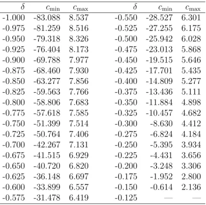
In Table 1, we tabulate the values of_c∈(_{cmin, cmax}) for which the size of the right-tailed

t-test exceeds 7_.5%, for selected values of _δ. For instance, when _δ = −0_.95, the nominal 5% _t-test has asymptotic size greater than 7.5% if _c ∈ (−79_.318_,8_.326). The table can be used to construct a pretest to determine whether inference based on the conventional_t-test is sufficiently reliable.

Suppose a researcher is willing to tolerate an actual size of up to 7.5% for a nominal 5% test of predictability. To test the null hypothesis that the actual size exceeds 7.5%, we first construct a 100(1−_α1)% confidence interval for _c and estimate _δ using the residuals from regressions (1) and (2).4 We reject the null if the confidence interval for _clies strictly below (or above) the region of the parameter space (_{cmin, cmax}) where size distortion is large. The relevant region (_{cmin, cmax}) is determined by Table 1, using the value of _δ that is closest to the estimated correlation_δ. As emphasized by Elliott and Stock (1994), the rejection of the unit root hypothesis _c = 0 is not sufficient to assure that the size distortion is acceptably small. Asymptotically, this pretest has size _α1.

In our empirical application, we construct the confidence interval for _c by applying the method of confidence belts as suggested by Stock (1991). The basic idea is to compute a unit root test statistic in the data and to use the known distribution of that statistic under the alternative to construct the confidence interval for _c. A relatively accurate confidence interval can be constructed by using a relatively powerful unit root test (Elliott and Stock, 2001). We therefore use the Dickey-Fuller generalized least squares (DF-GLS) test of Elliott et al. (1996), which is more powerful than the commonly used augmented Dickey-Fuller (ADF) test. The idea behind the DF-GLS test is that it exploits the knowledge _ρ ≈ 1 to obtain a more efficient estimate of the intercept _γ.5 We refer to Campbell and Yogo (2005) for a detailed description of how to construct the confidence interval for_cusing the DF-GLS

4_{When the predictor variable is generalized to an AR(p), the residual is that of regression (23) in Appendix}

A.

5_{A note of caution regarding the DF-GLS confidence interval is that the procedure might not be valid}

whenρ1 (since it is based on the assumption thatρ≈1). In practical terms, this method should not be used on variables that would not ordinarily be tested for an autoregressive unit root.

statistic.

3.3.

Making tests feasible by the Bonferroni method

As discussed in Section 3.1, both the_t-test and the_Q-test are infeasible since the procedures depend on an unknown nuisance parameter_c, which cannot be estimated consistently. Intu-itively, the degree of persistence, controlled by the parameter _c, influences the distribution of test statistics that depend on the persistent predictor variable. This must be accounted for by adjusting either the critical values of the test (e.g., _t-test) or the value of the test statistic itself (e.g., _Q-test). Cavanagh et al. (1995) discuss several (sup-bound, Bonferroni, and Scheffe-type) methods of making tests that depend on_cfeasible.6 Here, we focus on the Bonferroni method.

To construct a Bonferroni confidence interval, we first construct a 100(1−_α1)% confidence interval for _ρ, denoted as _Cρ(_α1). (We parameterize the degree of persistence by _ρ rather than _c since this is the more natural choice in the following.) For each value of _ρ in the confidence interval, we then construct a 100(1−_α2)% confidence interval for _β given _ρ, denoted as _Cβ|ρ(_α2). A confidence interval that does not depend on _ρ can be obtained by

Cβ(α) =

ρ∈Cρ(α1)

Cβ|ρ(α2). (13)

By Bonferroni’s inequality, this confidence interval has coverage of at least 100(1−_α)%, where _α=_α1+_α2.

In principle, one can use any unit root test in the Bonferroni procedure to construct the confidence interval for _ρ. Based on work in the unit root literature, reasonable choices are the ADF test and the DF-GLS test. The DF-GLS test has the advantage of being more powerful than the ADF test, resulting in a tighter confidence interval for _ρ.

In the Bonferroni procedure, one can also use either the _t-test or the _Q-test to construct

6_{These are standard parametric approaches to the problem. For a nonparametric approach, see Campbell}

the confidence interval for _β given _ρ. We know that the_Q-test is a more powerful test than the _t-test when _ρ is known. In fact, it is UMP conditional on an ancillary statistic in that situation. This means that the conditional confidence interval_Cβ|ρ(_α2) based on the _Q-test is tighter than that based on the _t-test at the true value of _ρ. Without numerical analysis, however, it is not clear whether the _Q-test retains its power advantages over the _t-test at other values of _ρ in the confidence interval _Cρ(_α1).

In practice, the choice of the particular tests in the Bonferroni procedure should be dictated by the issue of power. Cavanagh et al. (1995) propose a Bonferroni procedure based on the ADF test and the _t-test. Torous et al. (2004) have applied this procedure to test for predictability in U.S. data. In this paper, we examine a Bonferroni procedure based on the DF-GLS test and the _Q-test. While there is no rigorous justification for our choice, our Bonferroni procedure turns out to have better power properties, which we show in Section 3.5.

Because the_Q-statistic is normally distributed, and the estimate of_β declines linearly in

ρ when _δ is negative, the confidence interval for our Bonferroni _Q-test is easy to compute. The Bonferroni confidence interval for_β runs from the lower bound of the confidence interval for_β, conditional on_ρequal to the upper bound of its confidence interval, to the upper bound of the confidence interval for _β, conditional on _ρ equal to the lower bound of its confidence interval. More formally, an equal-tailed _α2-level confidence interval for _β given _ρ is simply

Cβ|ρ(α2) = [β(ρ, α2), β(ρ, α2)], where β(_ρ) = _T t=1xµt−1[rt−βue(xt−ρxt−1)] _T t=1xµt−21 , (14) β(_{ρ, α2}) = _β(_ρ)−_zα2/2σu 1−_δ2 _T t=1xµt−21 1/2 , (15) β(_{ρ, α2}) = _β(_ρ) +_zα2/2σu 1−_δ2 _T t=1xµt−21 1/2 , (16)

[_ρ(_α1)_{, ρ}(_α1)] denote the confidence interval for _ρ, where _α1 = Pr(_{ρ < ρ}(_α1)), _α1 = Pr(_{ρ >}

ρ(_α1)), and _α1 =_α1+_α1. Then the Bonferroni confidence interval is given by

Cβ(α) = [β(ρ(α1), α2), β(ρ(α1), α2)]. (17)

In Campbell and Yogo (2005), we lay out the step-by-step recipe for implementing this confidence interval in the empirically relevant case when the nuisance parameters (i.e., _σu,

δ, and _βue) are not known.

3.4.

A refinement of the Bonferroni method

The Bonferroni confidence interval can be conservative in the sense that the actual coverage rate of _Cβ(_α) can be greater than 100(1−_α)%. This can be seen from the equality

Pr(_β ∈_Cβ(_α)) = Pr(_β ∈_Cβ(_α)|_ρ ∈_Cρ(_α1)) Pr(_ρ∈_Cρ(_α1)) + Pr(_β ∈_Cβ(_α)|_ρ∈_Cρ(_α1)) Pr(_ρ∈_Cρ(_α1))_.

Since Pr(_β ∈ _Cβ(_α)|_ρ ∈ _Cρ(_α1)) is unknown, the Bonferroni method bounds it by one as the worst case. In addition, the inequality Pr(_β ∈ _Cβ(_α)|_ρ ∈ _Cρ(_α1)) ≤ _α2 is strict unless the conditional confidence intervals _Cβ|ρ(_α2) do not depend on _ρ. Because these worst case conditions are unlikely to hold in practice, the inequality

Pr(_β ∈_Cβ(_α))≤_α2(1−_α1) +_α1 ≤_α

is likely to be strict, resulting in a conservative confidence interval.

Cavanagh et al. (1995) therefore suggest a refinement of the Bonferroni method that makes it less conservative than the basic approach. The idea is to shrink the confidence interval for_ρso that the refined interval is a subset of the original (unrefined) interval. This consequently shrinks the Bonferroni confidence interval for_β, achieving an exact test of the

desired significance level. Call this significance level_α, which we must now distinguish from

α=_α1+_α2, the sum of the significance levels used for the confidence interval for _ρ(denoted

α1) and the conditional confidence intervals for _β (denoted _α2).

To construct a test with significance level _α, we first fix _α2. Then, for each _δ, we numerically search to find the _α1 such that

Pr(_β(_ρ(_α1)_{, α2})_{> β})≤_α/ 2 (18)

holds for all values of _con a grid, with equality at some point on the grid. We then repeat the same procedure to find the _α1 such that

Pr(_β(_ρ(_α1)_{, α2})_{< β})≤_α/ 2_. (19)

We use these values _α1 and _α1 to construct a tighter confidence interval for_ρ. The resulting one-sided Bonferroni test has exact size _α/ 2 for some permissible value of _c. The resulting two-sided test has size at most_α for all values of_c.

In Table 2, we report the values of_α1 and_α1 for selected values of_δwhen_α=_α2 = 0_.10, computed over the grid _c∈ [−50_,5]. The table can be used to construct a 10% Bonferroni confidence interval for _β (equivalently, a 5% one-sided _Q-test for predictability). Note that

α₁ and _α1 are increasing in_δ, so the Bonferroni inequality has more slack and the unrefined Bonferroni test is more conservative the smaller is_δ in absolute value. In order to implement the Bonferroni test using Table 2, one needs the confidence belts for the DF-GLS statistic. Campbell and Yogo (2005, Tables 2–11) provide lookup tables that report the appropriate confidence interval for _c, _Cc(_α1) = [_c(_α1)_{, c}(_α1)], given the values of the DF-GLS statistic and_δ. The confidence interval_Cρ(_α1) = 1 +_Cc(_α1)_/T for_ρthen results in a 10% Bonferroni confidence interval for _β.

Our computational results indicate that in general the inequalities (18) and (19) are close to equalities when _c≈ 0 and have more slack when _c 0. For right-tailed tests, the

probability (18) can be as small as 4.0% for some values of _cand _δ. For left-tailed tests, the probability (19) can be as small as 1.2%. This suggests that even the adjusted Bonferroni

Q-test is conservative (i.e., undersized) when _{c <} 5. The assumption that the predictor variable is never explosive (i.e., _c ≤ 0) would allow us to further tighten the Bonferroni confidence interval. In our judgment, however, the magnitude of the resulting power gain is not sufficient to justify the loss of robustness against explosive roots. (The empirical relevance of allowing for explosive roots is discussed in Section 4.)

3.5.

Power under local-to-unity asymptotics

Any reasonable test, such as the Bonferroni _t-test, rejects alternatives that are a fixed dis-tance from the null with probability one as the sample size becomes arbitrarily large. In practice, however, we have a finite sample and are interested in the relative efficiency of test procedures. A natural way to evaluate the power of tests in finite samples is to consider their ability to reject local alternatives.7 When the predictor variable contains a local-to-unit root, OLS estimators_βand _ρare consistent at the rate _T (rather than the usual √_T). We therefore consider a sequence of alternatives of the form _β = _β0 +_b/T for some fixed constant _b. The empirically relevant region of _b for the dividend-price ratio, based on OLS estimates of_β, appears to be the interval [8_,10], depending on frequency of the data (annual to monthly). Details on the computation of the power functions are in Appendix B.

3.5.1. Power of infeasible tests

We first examine the power of the _t-test and _Q-test under local-to-unity asymptotics. Al-though these tests assume knowledge of _c and are thus infeasible, their power functions provide benchmarks for assessing the power of feasible tests.

Fig. 3 plots the power functions for the _t-test (using the appropriate critical value that depends on _c) and the _Q-test. Under local-to-unity asymptotics, power functions are not

symmetric in _b. We only report the power for right-tailed tests (i.e., _{b >}0) since this is the region where the conventional _t-test is size distorted (recall the discussion in Section 3.2). The results, however, are qualitatively similar for left-tailed tests (available from the authors on request). We consider various combinations of _c(−2 and −20) and_δ (−0_.95 and−0_.75), which are in the relevant region of the parameter space when the predictor variable is a valuation ratio (see Table 4). The variances are normalized as _σ2_u =_σe2 = 1.

As expected, the power function for the _Q-test dominates that for the_t-test. In fact, the power function for the _Q-test corresponds to the Gaussian power envelope for conditional tests when_ρis known. In other words, the_Q-test has the maximum achievable power when_ρ is known and Assumption 1 holds. The difference is especially large when_δ=−0_.95. When the correlation between the innovations is large, there are large power gains from subtracting the part of the innovation to returns that is correlated with the innovation to the predictor variable.

To assess the importance of the power gain, we compute the Pitman efficiency, which is the ratio of the sample sizes at which two tests achieve the same level of power (e.g., 50%) along a sequence of local alternatives. Consider the case _c= −2 and _δ = −0_.95. To compute the Pitman efficiency of the _t-test relative to the _Q-test, note first that the _t-test achieves 50% power when_b = 4_.8. On the other hand, the _Q-test achieves 50% power when

b= 1_.8. Following the discussion in Stock (1994, p. 2775), the Pitman efficiency of the_t-test relative to the _Q-test is 4_.8_/1_.8 ≈ 2_.7. This means that to achieve 50% power, the _t-test asymptotically requires 170% more observations than the _Q-test.

3.5.2. Power of feasible tests

We now analyze the power properties of several feasible tests that have been proposed. Fig. 3 reports the power of the Bonferroni_t-test (Cavanagh et al., 1995) and the Bonferroni_Q-test.8

8_{The refinement procedure described in Section 3.4 for the BonferroniQ-test with DF-GLS is also applied}

to the Bonferronit-test with ADF. The significance levelsα₁andα₁used in constructing the ADF confidence interval forρare chosen to result in a 5% one-sided test forβ, uniformly inc∈[−50,5].

In all cases considered, the Bonferroni_Q-test dominates the Bonferroni_t-test. In fact, the power of the Bonferroni _Q-test comes very close to that of the infeasible _t-test. The power gains of the Bonferroni _Q-test over the Bonferroni _t-test are larger the closer is_cto zero and the larger is_δ in absolute value. When_c=−2 and_δ =−0_.95, the Pitman efficiency is 1.24, which means that the Bonferroni _t-test requires 24% more observations than the Bonferroni

Q-test to achieve 50% power.

In addition to the Bonferroni tests, we also consider the power of Lewellen’s (2004) test. In our notation (17), Lewellen’s confidence interval corresponds to [_β(1_{, α2})_{, β}(1_{, α2})]. Formally, this test can be interpreted as a sup-bound _Q-test, that is, the _Q-test that sets _ρ equal to the value that maximizes size. The value _ρ = 1 maximizes size, provided that the parameter space is restricted to _ρ ≤ 1, since _Q(_{β0, ρ}) is decreasing in _ρ when _{δ <} 0. By construction, the sup-bound _Q-test is the most powerful test when _c = 0. When _c = −2 and _δ = −0_.95, the sup-bound _Q-test is undersized when _b is small and has good power when _b 0. When _c =−2 and _δ = −0_.75, the power of the sup-bound _Q-test is close to that of the Bonferroni _Q-test. When_c=−20, the sup-bound _Q-test has very poor power.9 In some sense, the comparison of the sup-bound _Q-test with the Bonferroni tests is unfair because the size of the sup-bound test is greater than 5% when the true autoregressive root is explosive (i.e.,_{c >} 0), while the Bonferroni tests have the correct size even in the presence of explosive roots.

We conclude that the Bonferroni _Q-test has important power advantages over the other feasible tests. Against right-sided alternatives, it has better power than the Bonferroni _t -test, especially when the predictor variable is highly persistent, and it has much better power than the sup-bound _Q-test when the predictor variable is less persistent.

9_{Lewellen (2004, Section 2.4) proposes a Bonferroni procedure to remedy the poor power of the}

sup-boundQ-test for low values ofρ. Although the particular procedure that he proposes does not have correct asymptotic size (see Cavanagh et al., 1995), it can be interpreted as a combination of the Bonferronit-test and the sup-boundQ-test.

3.5.3. Where does the power gain come from?

The last section showed that our Bonferroni _Q-test is more powerful than the Bonferroni

t-test. In this section, we examine the sources of this power gain in detail. We focus our discussion of power to the case _δ =−0_.95 since the results are similar when _δ =−0_.75.

We first ask whether the power gain comes from the use of the DF-GLS test rather than the ADF test, or the_Q-test rather than the_t-test. To answer this question, we consider the following three tests:

1. A Bonferroni test based on the ADF test and the _t-test. 2. A Bonferroni test based on the DF-GLS test and the _t-test. 3. A Bonferroni test based on the DF-GLS test and the _Q-test.

Tests 1 and 3 are the Bonferroni _t-test and _Q-test, respectively, whose power functions are discussed in the last section. Test 2 is a slight modification of the Bonferroni _t-test, whose power function appears in an earlier version of this paper (Campbell and Yogo, 2002, Fig. 5). By comparing the power of tests 1 and 2, we quantify the marginal contribution to power coming from the DF-GLS test. By comparing the power of tests 2 and 3, we quantify the marginal contribution to power coming from the Q-test.

When _c = −2 and _δ = −0_.95, the Pitman efficiency of test 1 relative to test 2 is 1.03, which means that test 1 requires 3% more observations than test 2 to achieve 50% power. The Pitman efficiency of test 2 relative to test 3 is 1.20 (i.e., test 2 requires 20% more observations). This shows that when the predictor variable is highly persistent, the use of the _Q-test rather than the _t-test is a relatively important source of power gain for the Bonferroni _Q-test.

When _c = −20 and _δ = −0_.95, the Pitman efficiency of test 1 relative to test 2 is 1.07 (i.e., test 1 requires 7% more observations). The Pitman efficiency of test 2 relative to test 3 is 1.03 (i.e., test 2 requires 3% more observations). This shows that when the predictor

variable is less persistent, the use of the DF-GLS test rather than the ADF test is a relatively important source of power gain for the Bonferroni _Q-test.

We now ask whether the refinement to the Bonferroni test, discussed in Section 3.4, is an important source of power. To answer this question, we recompute the power functions for the Bonferroni _t-test and _Q-test, reported in Fig. 3, without the refinement. Although these power functions are not directly reported here to conserve space, we summarize our findings.

When _c = −2 and _δ = −0_.95, there is essentially no difference in power between the unrefined and refined Bonferroni _t-test. However, the Pitman efficiency of the unrefined relative to the refined Bonferroni_Q-test is 1.62. When _c=−20 and_δ =−0_.95, the Pitman efficiency of the unrefined relative to the refined Bonferroni _t-test is 1.23. For the Bonferroni

Q-test, the corresponding Pitman efficiency is 1.55. This shows that the refinement is an especially important source of power gain for the Bonferroni_Q-test. Since the_Q-test explic-itly exploits information about the value of _ρ, its confidence interval for _β given _ρ is very sensitive to _ρ, resulting in a rather conservative Bonferroni test without the refinement.

3.6.

Finite-sample rejection rates

The construction of the Bonferroni _Q-test in Section 3.3 and the power comparisons of various tests in the previous section are based on local-to-unity asymptotics. In this section, we examine whether the asymptotic approximations are accurate in finite samples through Monte Carlo experiments.

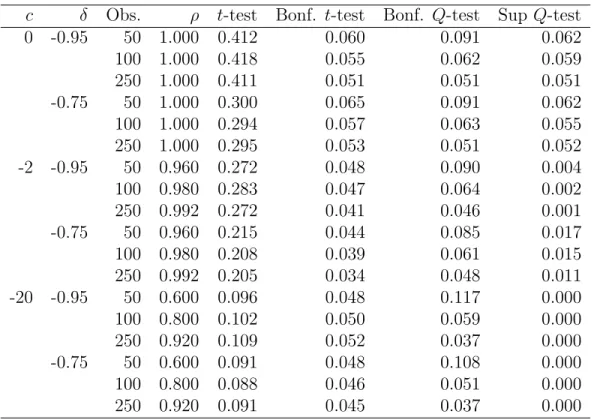
Table 3 reports the finite-sample rejection rates for four tests of predictability: the con-ventional _t-test, the Bonferroni _t-test, the Bonferroni _Q-test implemented as described in Campbell and Yogo (2005), and the sup-bound _Q-test. All tests are evaluated at the 5% significance level, where the null hypothesis is_β = 0 against the alternative_{β >}0. The rejec-tion rates are based on 10,000 Monte Carlo draws of the sample path using the model (1)–(2), with the initial condition _x0 = 0. The nuisance parameters are normalized as _α = _γ = 0

and _σ2_u =_σe2 = 1. The innovations have correlation_δand are drawn from a bivariate normal distribution. We report results for three levels of persistence (_c = {0_,−2_,−20}) and two levels of correlation (_δ ={−0_.95_,−0_.75}). We consider fairly small sample sizes of 50, 100, and 250 since local-to-unity asymptotics are known to be very accurate for samples larger than 500 (e.g., see Chan, 1988).

The conventional _t-test (using the critical value 1.645) has large size distortions, as re-ported in Elliott and Stock (1994) and Mankiw and Shapiro (1986). For instance, the rejection probability is 27.2% when there are 250 observations, _ρ = 0_.992, and _δ = −0_.95. On the other hand, the finite-sample rejection rate of the Bonferroni_t-test is no greater than 6.5% for all values of _ρ and _δ considered, which is consistent with the findings reported in Cavanagh et al. (1995).

The Bonferroni _Q-test has a finite-sample rejection rate no greater than 6.4% for all levels of _ρ and _δ considered, as long as the sample size is at least 100. The test does seem to have higher rejection rates when the sample size is as small as 50, especially when the degree of persistence is low (i.e., _c=−20). Practically, this suggests caution in applying the Bonferroni _Q-test in very small samples such as postwar annual data, although the test is satisfactory in sample sizes typically encountered in applications. The sup-bound _Q-test is undersized when _{c <}0, which translates into loss of power as discussed in the last section.

To check the robustness of our results, we repeat the Monte Carlo exercise under the assumption that the innovations are drawn from a_t-distribution with five degrees of freedom. The excess kurtosis of this distribution is nine, chosen to approximate the fat tails in returns data; the estimated kurtosis is never greater than nine in annual, quarterly, or monthly data. The rejection rates are essentially the same as those in Table 3, implying robustness of the asymptotic theory to fat-tailed distributions. The results are available from the authors on request.

As an additional robustness check, we repeat the Monte Carlo exercise under different assumptions about the initial condition. With _c = −20 and the initial condition _x0 =

{−2_,2}, the Bonferroni _Q-test is conservative in the sense that its rejection probability is lower than those reported in Table 3. With _c = {−2_,−20} and the initial condition _x0 drawn from its unconditional distribution, the Bonferroni _Q-test has a rejection probability that is slightly lower (at most 2% lower) than those reported in Table 3. To summarize, the Bonferroni_Q-test has good finite-sample size under reasonable assumptions about the initial condition.

4.

Predictability of stock returns

In this section, we implement our test of predictability on U.S. equity data. We then relate our findings to previous empirical findings in the literature.

4.1.

Description of data

We use four different series of stock returns, dividend-price ratio, and earnings-price ratio. The first is annual S&P 500 index data (1871–2002) from Global Financial Data since 1926 and from Shiller (2000) before then. The other three series are annual, quarterly, and monthly NYSE/AMEX value-weighted index data (1926–2002) from the Center for Research in Security Prices (CRSP).

Following Campbell and Shiller (1988), the dividend-price ratio is computed as dividends over the past year divided by the current price, and the earnings-price ratio is computed as a moving average of earnings over the past ten years divided by the current price. Since earn-ings data are not available for the CRSP series, we instead use the corresponding earnearn-ings- earnings-price ratio from the S&P 500. Earnings are available at a quarterly frequency since 1935, and an annual frequency before then. Shiller (2000) constructs monthly earnings by linear extrapolation. We instead assign quarterly earnings to each month of the quarter since 1935 and annual earnings to each month of the year before then.

rate for the monthly series and the three-month T-bill rate for the quarterly series. For the annual series, the risk-free return is the return from rolling over the three-month T-bill every quarter. Since 1926, the T-bill rates are from the CRSP Indices database. For our longer S&P 500 series, we augment this with U.S. commercial paper rates (New York City) from Macaulay (1938), available through NBER’s webpage.

For the three CRSP series, we consider the subsample 1952–2002 in addition to the full sample. This allows us to add two additional predictor variables, the three-month T-bill rate and the long-short yield spread. Following Fama and French (1989), the long yield used in computing the yield spread is Moody’s seasoned Aaa corporate bond yield. The short rate is the one-month T-bill rate. Although data are available before 1952, the nature of the interest rate is very different then due to the Fed’s policy of pegging the interest rate. Following the usual convention, excess returns and the predictor variables are all in logs.

4.2.

Persistence of predictor variables

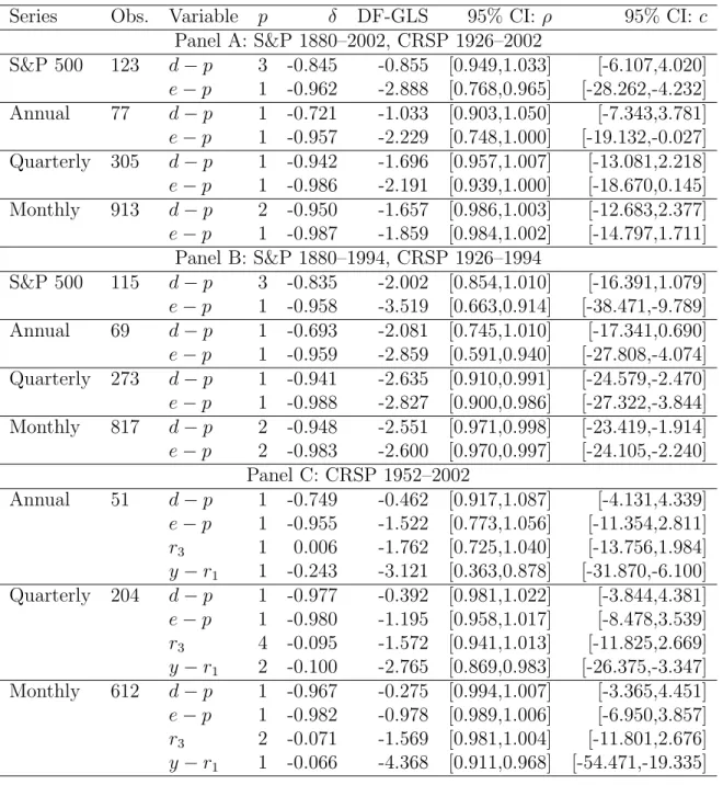
In Table 4, we report the 95% confidence interval for the autoregressive root _ρ (and the corresponding_c) for the log dividend-price ratio (_d−_p), the log earnings-price ratio (_e−_p), the three-month T-bill rate (_r3), and the long-short yield spread (_y−_r1). The confidence interval is computed by the method described in Section 3.2. The autoregressive lag length

p ∈ [1_{, p}] for the predictor variable is estimated by the Bayes Information Criterion (BIC). We set the maximum lag length_pto four for annual, six for quarterly, and eight for monthly data. The estimated lag lengths are reported in the fourth column of Table 4.

All of the series are highly persistent, often containing a unit root in the confidence interval. An interesting feature of the confidence intervals for the valuation ratios (_d−_p and _e−_p) is that they are sensitive to whether the sample period includes data after 1994. The confidence interval for the subsample through 1994 (Panel B) is always less than that for the full sample through 2002 (Panel A). The source of this difference can be explained by Fig. 1, which is a time-series plot of the valuation ratios at quarterly frequency. Around

1994, these valuation ratios begin to drift down to historical lows, making the processes look more nonstationary. The least persistent series is the yield spread, whose confidence interval never contains a unit root.

The high persistence of these predictor variables suggests that first-order asymptotics, which implies that the _t-statistic is approximately normal in large samples, could be mis-leading. As discussed in Section 3.2, whether conventional inference based on the _t-test is reliable also depends on the correlation _δ between the innovations to excess returns and the predictor variable. We report point estimates of _δ in the fifth column of Table 4. As expected, the correlations for the valuation ratios are negative and large. This is because movements in stock returns and these valuation ratios mostly come from movements in the stock price. The large magnitude of _δ suggests that inference based on the conventional

t-test leads to large size distortions.

Suppose _δ = −0_.9, which is roughly the relevant value for the valuation ratios. As reported in Table 1, the unknown persistence parameter_cmust be less than−70 for the size distortion of the _t-test to be less than 2.5%. That corresponds to _ρless than 0.09 in annual data, less than 0.77 in quarterly data, and less than 0.92 in monthly data. More formally, we fail to reject the null hypothesis that the size distortion is greater than 2.5% using the pretest described in Section 3.2. For the interest rate variables (_r3 and _y−_r1), _δ is much smaller. For these predictor variables, the pretest rejects the null hypothesis, which suggests that the conventional _t-test leads to approximately valid inference.

4.3.

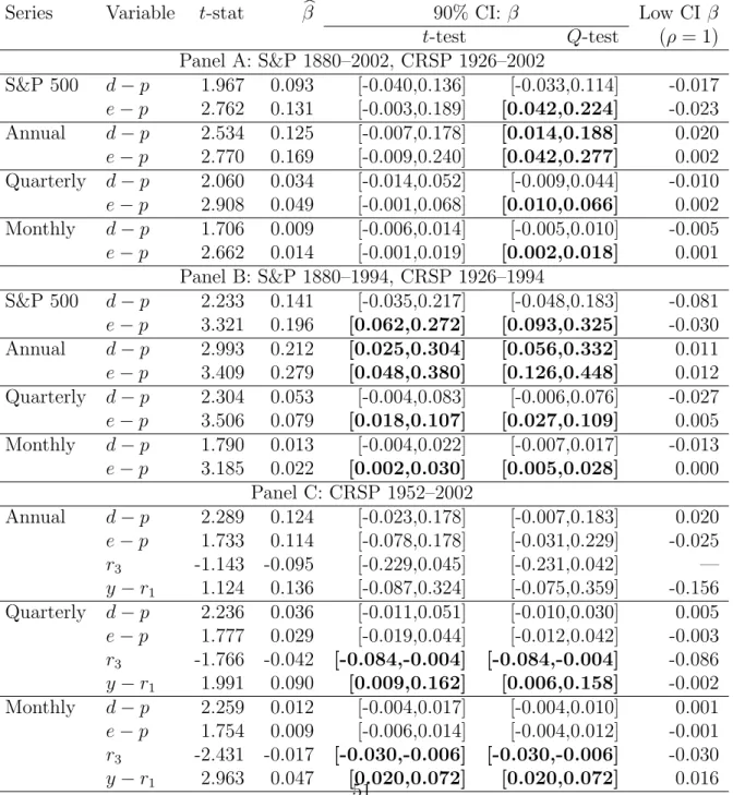
Testing the predictability of returns

In this section, we construct valid confidence intervals for _β through the Bonferroni _Q-test to test the predictability of returns. In reporting our confidence interval for _β, we scale it by _σe/σu. In other words, we report the confidence interval for _β= (_σe/σu)_β instead of _β. Although this normalization does not affect inference, it is a more natural way to report the empirical results for two reasons. First, _βhas a natural interpretation as the coefficient