Estimating arterial traffic conditions using sparse probe data
Ryan Herring
Industrial Engineering and Operations Research University of California, Berkeley
Aude Hofleitner
Electrical Engineering and Computer Science University of California, Berkeley
Pieter Abbeel
Electrical Engineering and Computer Science University of California, Berkeley
Alexandre Bayen
Civil and Environmental Engineering Systems Engineering University of California, Berkeley
Abstract
Estimating and predicting traffic conditions in arterial networks using probe data has proven to be a substantial challenge. In the United States, sparse probe data repre-sents the vast majority of the data available on arterial roads in most major urban environments. This article proposes a probabilistic modeling framework for estimating and pre-dicting arterial travel time distributions using sparsely ob-served probe vehicles.
We evaluate our model using data from a fleet of 500 taxis in San Francisco, CA, which send GPS data to our server every minute. The sampling rate does not provide detailed information about where vehicles encountered de-lay or the reason for any dede-lay (i.e. signal dede-lay, congestion delay, etc.). Our model provides an increase in estimation accuracy of 35% when compared to a baseline approach for processing probe vehicle data.
1. Introduction
Traffic congestion has a significant impact on economic activity throughout much of the world. An essential step towards active congestion control is the creation of accurate, reliable traffic monitoring systems.
Historically, traffic monitoring systems have been mostly limited to highways and have relied on public or private data feeds from a dedicated sensing infrastructure, which often includes loop detectors, radars, video cameras. For highway networks covered by such an infrastructure, it has become common practice to perform both system iden-tification of highway parameters (free flow speed, traffic jam density and flow capacity) and estimation of traffic state (flow, density, length of queues, bulk speed and shockwave location) at a very fine spatio-temporal scale [23, 4]. These highway traffic monitoring approaches heavily rely upon both the ubiquity of data and highway traffic flow models developed over the last half century [16, 6, 21].
For arterials (the secondary network) and highways not covered by dedicated sensing infrastructure, traffic monitor-ing is substantially more difficult: probe vehicle data is the only significant data source available today with the prospect
Figure 1. San Francisco taxi measurement locations for a single day, observed at a rate of once per minute.
of global coverage in the future. The features of probe ve-hicle data today, including the lack of ubiquity and relia-bility, the variety of data types and specifications, and the randomness of its spatio-temporal coverage, make it insuffi-cient for fully characterizing macroscopic traffic model pa-rameters and doing state estimation with these models for large transportation networks. Figure 1 shows probe mea-surements from San Francisco taxis for one day, which il-lustrates the breadth of coverage when aggregating data over longer periods of time. However, this data does not pro-vide enough information to directly infer the macroscopic state of traffic at a fine spatio-temporal scale. Traffic models and data assimilation algorithms must be developed to effi-ciently transform this data into reliable traffic information. See, e.g., [23, 22, 11, 14] for a discussion on the use of cell phone data for highway traffic monitoring.
Aside from less abundant sensing compared to exist-ing highway traffic monitorexist-ing systems, the arterial network presents additional modeling and estimation challenges as the underlying flow physics which governs them is more
complex because of traffic lights (often with unknown cy-cles), intersections, stop signs, parallel queues, and others. Collecting the detailed parameters of the arterial road net-work into an accessible electronic database would require the cooperation of numerous government agencies, making this information unreliable and tedious to obtain. Moreover, at the low penetration rate typical for arterial traffic, even small changes in the road network can greatly affect the es-timation. This makes the detailed spatio-temporal modeling and estimation approaches developed for highway traffic im-practical for arterials—at least until the data volume signifi-cantly increases [3, 18].
We propose a statistical approach for arterial traffic esti-mation from probe vehicle data by modeling the evolution of trafficstatesas aCoupled Hidden Markov Model(CHMM), which is a particular form of a probabilistic graphical model. Our approach starts from well established first principle traf-fic flow models for arterial traftraf-fic [16, 20]. We then show how these traffic flow models can be leveraged to estimate historical travel time probability distributions as well as pre-dict the short-term evolution of travel times.
CHMMs have been used for predicting the evolution of sensor readings on highways [15]. The approach in [15] re-lies on the fact that fixed infrastructure sensors (loop detec-tors) provide exactly one measurement every 30 seconds at a fixed location. Probe data on arterials is available at random times and random locations, making this model not applica-ble for our study. Statistical approaches have been proposed that rely on either a single measurement per time interval or aggregated measurements per time interval [10, 8], neither of which is appropriate in our setting. Another probabilis-tic graphical model approach based on the statisprobabilis-tical physics Ising model was proposed in [8]. This model relies on mea-suring a binary quantity stating whether traffic is congested or uncongested. Transforming probe data into binary con-gested/uncongested values is a difficult process by itself and has not been specifically addressed to our knowledge.
Some researchers have examined the case of how to pro-cess high-frequency probe data (one measurement approxi-mately every 20 seconds or less) [22]. High-frequency data allows for reliable calculation of short distance speeds and travel times. In this paper, we specifically address the pro-cessing of sparse probe data where this level of granular-ity is not available. Finally, other approaches based on re-gression [17], optimization [2], neural networks and pattern matching [7] have all been proposed. None of these ap-proaches addresses the issue of processing sparse probe data on a dense arterial network. Hellinga, et al. [9], address the case of low frequency sampled probe data. In that paper, the authors construct a simple probability function with intuitive properties, but the approach is not based on traffic theory as is our approach in this paper.
The contribution of our work specifically addresses the case of noisy, sparse probe data. In particular, we propose a model and algorithm to do traffic estimation with mea-surements received atrandom locationsandrandom times.
We define the travel time distribution of each observation (time between consecutive measurements) as a function of (i) the travel time distributions of the links traversed and (ii) the spatial distribution of vehicle locations on each traversed link. The key insight is that, on average, vehicles spend more time traveling through the part of a link just before an inter-section than they spend on the part of a link just after an intersection (section 2). Based on traffic modeling assump-tions, we construct a graphical model (section 3) represent-ing the travel time distribution of each link at each time in-terval and their spatio-temporal evolution. Leveraging the results from section 2, the graphical model represents travel time distributions on any portion of the links of the network (partial links) and estimates the probability of an observa-tion given travel time distribuobserva-tion parameters. We develop anexpectation maximization(EM) algorithm (section 4) for learning the parameters of our CHMM. We estimate the cur-rent state of the network using a particle filter, which is used for predicting the link travel time distributions in the short-term future. Finally, we present the results of a case study (section 5) in San Francisco, for which a fleet of 500 taxis provides sparse location measurements as part of the Mo-bile Millenniumproject [12]. The initial results indicate that travel time distributions can be accurately estimated using only sparse GPS data.
2. Traffic modeling framework
We present the assumptions and notations of a model of traffic through a signalized intersection. Given these as-sumptions, we derive travel time distributions between any two points of the network based on the spatial distribution of vehicles along each link of the path. This provides a frame-work for computing the likelihood of a probe vehicle obser-vation given the parameters of the network.
2.1. Traffic modeling assumptions
To model traffic dynamics, we use the following set of model parameters: maximum densityρmax, critical density ρc, free flow speedvf, cycle timeC and red timeR. The demand in traffic is represented by the arrival density on a link, ρa. These parameters are defined for each linkl and each dayd. For simplicity of notations, we omit to write the dependency on the linkland the dayd.
We denoteNln the spatial neighbors of linkl of order n, where first order neighbors (Nl1) are the links sharing an intersection with linkl (including linkl). The higher order spatial neighbors are defined by the following recursive for-mula:
Nln+1= [
j∈Nl n
N1j (1)
To formulate our model, we make the following as-sumptions:
1. Triangular fundamental diagram.
2. Stationarity of traffic: during each estimation interval, the parameters of the light cycles (red and cycle time) do not change. The arrival densityρais constant. The
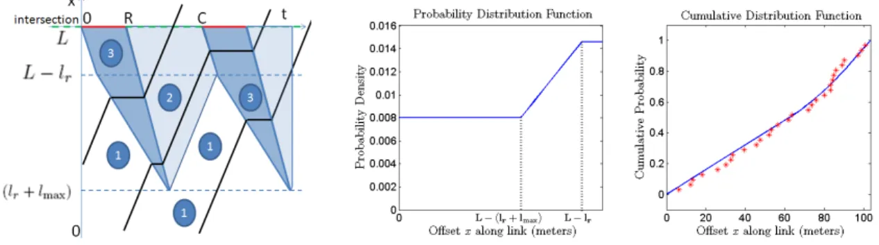
Figure 2. The estimation of the spatial distribution of vehicles on a link as derived from the model of traffic. The space-time plane is used to represent the density of vehicles (left). Using a maximum likelihood estimation, we derive the parameters of the model. The probability density at locationx(center) and the estimated and empirical cumulative distribution of the vehicle locations (right) demonstrate that the data fit the model assumptions well. The data used are on one link of the San Francisco network from a single time interval (5:00pm-5:30pm) aggregated over 20 days.
traffic dynamics are stationary: they evolve periodically with periodC(length of the light cycle). In particular, there is no consistent increase or decrease in the length of the queue, or instability.
3. First In First Out(FIFO) model: overtaking on the road network is neglected.
4. Discrete congestion states: for each day d and each time intervalt, the traffic conditions on linkl are rep-resented by a discretevalue,sld,t, which indicates the level of congestion. There areSdiscrete levels of con-gestion.
5. Conditional independence of link travel times: condi-tioned on the statesl
d,t of a linkl, the travel time distri-bution of that link is independent from all other traffic variables.
6. Conditional independence of state transitions: condi-tioned on the states of the spatial neighbors of linklof ordern(denotedNl
n) at timet, the state of linklat time t+1 is independent from all other current link states, all past link states and all past travel time observations. Assumption 5 implies that link travel times are not cor-related across links, which is an assumption made for com-putational tractability. Assumption 6 implies that each link is correlated with some (small) subset of neighboring links, but independent of the rest of the network. Neither of these as-sumptions must hold all of the time in a real traffic network, although it is our belief that this is a good approximation. Future studies will examine the extent to which this approx-imation affects the results and whether these assumptions can be relaxed while still having a model that is tractable to solve.
2.2. Path travel time probability distribution
As the location measurements are taken uniformly over time, more densely populated areas of the link will have more location measurements. We estimate the probability distribution PX of vehicle locations within a link using a
statistical model derived from traffic theory and modeling assumptions 1, 2, and 3. For a vehicle traveling from loca-tionx1to locationx2on an arterial linkl, we assume that the partial travel timeYx1,x2is distributed asαx1,x2Yl, whereYl is
the random variable of travel time on linkl—with realiza-tions denotedyl—and
αx1,x2=
Z x2 x1
PX(x)dx. (2)
Note that a baseline approach would assume thatαx1,x2
is the ratio between the distance|x2−x1|and the length of the link, assuming that the travel time on a link is uniformly distributed on the link. Our model takes into account the non spatial uniformity of travel time along a link of the network.
Probability distribution of vehicle locations. On a road
segment, at a locationxand a timet, the density takes one of the following values: (1) arrival densityρafor the vehicles that are upstream of the queue, (2) maximum densityρmax for the vehicles stopped at timetand locationxand (3) crit-ical densityρc for the vehicles downstream of the queue— vehicles that have already stopped on their trajectory on link l. These different values of the density at locationxand time t are represented in the space-time diagram of trajectories (Figure 2, left). In a stationary regime, we define the tri-angular queue (from its tritri-angular shape on the space-time diagram of trajectories) as the spatio-temporal region where vehicles stop for the first time on the link. Its length is called the maximum queue length, denotedlmax. Under congested conditions, the part of the queue downstream of the triangu-lar queue, called theremaining queuewith lengthlr, corre-sponds to vehicles which have to stop more than once be-fore going through the intersection. In a stationary regime, we can define the temporal average density at locationx, de-notedd(x). It is constant upstream of the maximum queue length—equal toρa. It increases linearly until the beginning of the remaining queuelr. In the remaining queue, the den-sity is constant, equal to ρb. The density ρb is computed as a convex combination of the maximum densityρmaxand
the critical densityρc—the density at which the queue dis-charges. The weights are given by the proportion of the cycle experiencing each of the density, thus the expression forρb,
ρb=CRρmax+ (1− R C)ρc.
Remark: The model presented is not restrictive with re-spect to the presence of a remaining queue, which is only present under congested conditions. During undersaturated conditions, we havelr=0. In the triangular queue the den-sity increases linearly. The value of the denden-sity at the inter-section is computed as a convex combination ofρmax,ρcand
ρawhere the weights represent the fraction of the cycle dur-ing which each of the density is observed. The average den-sity at the intersection isρb=CRρmax+Cτρc+ (1−RC+τ)ρa, whereτis theclearing time—time during which the light is green and the queue is dissipating.
The probability distribution of vehicle locationsPX is proportional to the average density. The normalizing con-stantZis the average number of vehicles on the link
PX(x) = 1
Zd(x), (3)
withZ=RL
0 d(u)du.
After normalization the probability distributionPX(x) is equal to ˜ ρa, x∈[0,L−(lr+lmax)] ˜
ρa+ρ˜bx−(llrmax+lmax), x∈[L−(lr+lmax),L−lr] ˜
ρa+ρ˜b, x∈[L−lr,L],
(4)
where ˜ρa=ρaZ,Z=ρaL+12lmaxρb+lrρband ˜
ρb=ρb/Z=2 1 −ρa˜ L
lmax+2lr. The distribution is fully determined with the three parameters ˜ρa,lrandlmax.
We estimate the parameters of the distribution of vehi-cle location on a linkPX by maximizing the likelihood of the set of location observations (denoted(xo)o∈O). This op-timization problem is written in equation (5).
argmax ˜ ρa,lr,lmax o
∑
∈O ln(PX(xo)) s.t. 0≤ρ˜a≤1L lr+lmax≤L 0≤lr,0≤lmax (5)The constraints come from the physics of the problem. The first constraint can be rewritten asρa≤ZL, whereZL rep-resents the average density on the whole link. It illustrates the fact that the arrival density is inferior to the average den-sity on the link. The other constraints illustrate that the total queue cannot extend the length of the link and that the trian-gular queue and the remaining queue must be non-negative. Experimental results have shown that the model learns the parameters with a relatively small amount of data. An example of the learned and experimental cumulative distri-butions of vehicle location for a link of the network are rep-resented in figure 2 (right).
3. Modeling framework
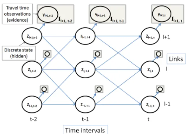
Arterial traffic conditions vary over space and time. Given assumptions 4, 5, and 6 in section 2.1, we model the spatio-temporal conditional dependencies of arterial traffic using a probabilistic graphical model known as a Coupled
Figure 3. Spatio-temporal model of arterial traffic evolution rep-resented as a coupled hidden Markov model. The circular nodes represent the (hidden) discrete state of traffic for each link at each time interval. The square nodes represent travel time ob-servations from the distribution defined by the traffic state.
Hidden Markov Model (CHMM) [5]. A Hidden Markov Model(HMM) is a statistical model in which the system be-ing modeled is assumed to be a Markov process with unob-served states. CHMMs model systems of multiple interact-ing processes. In this article, the multiple processes evolv-ing over time are the discretestates(assumption 4) of each link in the arterial network. Since we do not observe the state of each link for all times, these processes are consid-ered hidden. The travel time distribution on each link is conditioned on its hidden state (assumption 5) from which we have sparse observations from probe vehicles traveling through the arterial network. Assumption 6 gives the cou-pled structure to the HMM by specifying local dependen-cies between adjacent links of the road network. Figure 3 illustrates our model representation of link states and probe vehicle observations. Each circular node in the graph rep-resents the state of a link in the road network. The state is a discrete quantity defined based on the application (e.g. the possible states could be undersaturated/congested or the number of vehicles in the queue). The forward arrows in-dicate the local spatial dependency of links from one time period to the next. Each square node in the graph represents probe vehicle observations on the link to which it is attached (i.e. travel time between GPS measurements).
The observations are successive GPS measurements of vehicle trajectories (approximately one per minute). The is-sues of filtering the noise of the GPS to estimate the most likely location of the measurements and inferring the path taken by the vehicle are not addressed in this article. There are multiple approaches to solving this problem including using statistical filtering [13]. In the remainder of this ar-ticle, we assume that we are given the most likely measure-ment locations on the road network as well as the most likely path of the vehicle.
To completely specify the CHMM-based model, we have to estimate (i) the initial state probabilities for each link, denotedπl,s, (ii) the discrete transition probability
dis-tribution functions (assumption 6), denotedAl,t, and (iii) the distribution of travel time on a link given the state of that link (assumption 5), denotedgl,s,t.
For each linkland each time intervalt, the probability of linkl to be in statesat timet+1 given the state of its neighbors at timetis given by thediscrete transition proba-bility distributionfunction of linkl. It is fully characterized by a matrix of sizeSNln×S, denotedAl,t. The element of line rand columns,Al,t(r,s), represents the probability of linkl to be in statesat timet+1 given that the neighbors oflare in staterat timet.
A simplifying assumption for computational tractability is to assume that for each linkl, the state transition matrix Al,tand the conditional travel time distribution functiongl,s,t do not depend on time. They are denoted respectively byAl andgl,sin the reminder of this article. To relax this assump-tion, one can assume that these functions are piecewise con-stant in time and estimate them for each period of time dur-ing which the stationarity assumption is satisfied. We also assume that, given the state of a link, the travel time distri-bution on that link is independent from all the other random variables. In general, travel time distributions across links are not independent (due to light synchronization, platoons, and other factors). Future work will specifically address the challenge of using correlated distributions, which have the potential to capture more complex dynamics in the arterial road network.
4. Parameter estimation
In this section, we describe how the traffic modeling assumptions allow identification of the parameters of the model and the state variables using the path observations. Given the parameters of the model, we can estimate the most likely state of the links given observations and their evolu-tion over time. Similarly, given the state of the links of the network over a period of time, we can estimate the param-eters of the model (state transition matrix, and conditional travel time probability distributions). This well known type of problem is solved using an Expectation Maximization (EM) algorithm which iterates between finding the probabil-ity of each state for each link of the network and each time interval given some values of the model parameters (E step). Then, the probabilities of each state for each link and each time interval are used to update the value of the parameters by maximizing the log likelihood (M step).
One challenge of our graphical model approach is that we do not observe link travel times directly since the probe observations we receive can span several links of the net-work between two consecutive measurements. This diffi-culty is addressed by computing the most likely link travel times that make up the path of the probe vehicle (travel time allocation), which is described in section 4.1. It is possible to have a graphical model representation that does not have this decomposition approach, but it leads to a difficult non-linear parameter optimization (M-step) problem, for which the number of variables increase quadratically in the
num-ber of links. This optimization problem would require an approximation technique to solve, which is why we propose a more intuitive decomposition scheme calledtravel time al-location.
A high-level description of the parameter estimation is presented in Algorithm 1.
4.1. Travel time allocation
An observation consists of a travel time over a path con-sisting of multiple (partial) links. In order to use the graphi-cal model presented in section 3, the total travel time must be decomposed into a travel time for each (partial) link on the path. This can be achieved by maximizing the log-likelihood of the link travel times for each observation given the model parameters. This optimization problem for a single observa-tion is argmax y (
∑
l∈P ln( S∑
s=1 zslgl,s(yl)) :∑
l∈P αxl 1,xl2yl=y˜ ) , (6)wherePis the set of links on the path,y:={yl}l∈Pis a vec-tor of the travel times assigned to each link on the path,xl1 andxl2 are the start and end location on linkl, ˜yis the ob-served travel time between the GPS measurements, and zsl is the probability of linkl to be in state s. The values of xl1andxl2will be equal to the start and end of the link for all intermediate links and will only have non-trivial values for the first and last link of the path (where the actual GPS observations are). The values ofzsl are obtained from the E-step of the EM algorithm, except in the first iteration where they have been initialized with reasonable values (see Algo-rithm 1). The optimization problem in equation (6) has a number of variables equal to the number of links of the path between consecutive GPS measurements, which is always a relatively small number. This makes the optimization prob-lem easy to solve using numerical methods.
As a reminder, we use the density model of section 2 to computeαx1,x2, the proportion of the full link travel time to
use.
4.2. E step: Particle filtering
On small networks, it is possible to do exact inference in the CHMM by converting the model to an HMM with a state of dimension number of links. However, the transi-tion matrix is aSN×SN matrix (Nis the number of links in the network), which is intractable for any reasonable traffic network. Instead, we use an approximation based on parti-cle filtering. Each partiparti-cle represents an instantiation of the time evolution of the network. Each particle has a weight proportional to the probability of having this instantiation of the state evolution of the network given the available data. We simulate a high number of particles that evolve through the graphical model. These particles are used to estimate the probabilities of the state of each link and each time interval and the probabilities of transition between the state of the neighbors of link l at time t−1 and the state of linkl at timet. For more information on particle filtering, see, for example [19].
4.3. M step: Update of the parameters
For each link and each state, we assume that the travel time distributiongl,sis parameterized by a set of parameters pl,sand we note the set of all parametersP= (pl,s)l,s. To up-date these parameters, we maximize the expected complete log-likelihood given the expected values of the probabilities that each linklis in statesat timetand dayd(zsd,t,l) and the expected values of linklto be in statesgiven that the neigh-bors of link l are in staterat timet−1 and dayd (qsd,,rt,l). We also update the transition matricesAland the initial state probabilitiesπl for each link of the network, which corre-sponds to optimizing on the set of parametersA= (Al)land
π= (πl,s)l,s. The expected complete log likelihood is Λ(Y|z,q,P,A,π) = N
∑
l=1 S∑
s=1 D∑
d=1 Td∑
t=1 zsd,t,l Id,t,l∑
i=1 ln(gl,s(yi)) ! + N∑
l=1 D∑
d=1 Td∑
t=2 S∑
s=1 SNln∑
r=1 qsd,,rt,lln(Al(r,s)) + N∑
l=1 D∑
d=1 S∑
s=1 zsd,0,lln(πl,s), (7)whereId,t,l is the set of travel time observations for day d, time intervalt, and linklas provided by the travel time allo-cation method presented in section 4.1.
The usual optimization problem is modified to take into account the varying number of observations for each link and each time interval. The optimization problem is stated as max P,A Λ(Y|z,q,P,A,π) : S ∑ s=1 Al(r,s) =1,∀l,r Al(r,s)∈[0,1],∀l,r,s S ∑ s=1 πl,s=1,∀l πl,s∈[0,1],∀l,s (8) The updates of the transition probabilitiesAland of the initial state probabilitiesπl are straightforward. The update of the travel time distributions depends on the type of distri-bution used in the model. Due to the travel time allocation, the optimization problem on all the parametersPof the net-work decouples inS×Nsmaller optimization problems, one for each state and link of the network. For statesand linkl, the optimization problem is
max pl,s D ∑ d=1 Td ∑ t=1 zsd,t,l Id,t,l ∑ i=1 ln(gl,s(yi)) ! , (9)
wherepl,srepresents the parameters of the travel time distri-butiongl,s. Decoupling the optimization problem makes it highly scalable as each of the optimization subproblems can be performed in parallel. If the travel time allocation method is not used, then the resulting optimization problem is cou-pled across the whole network resulting in a large non-linear optimization problem that does not scale well.
Algorithm 1 Estimation of the historical distribution of
travel time and state transition probability matrices. Estimate the link parameters for the density model (sec-tion 2.2)
Initialize the parametersPl,s of the distributions, the state transition probability matricesAl, the initial state proba-bilitiesπl,s, and the state probabilitieszsd,t,l
EM-algorithm with travel time allocation:
whileThe algorithm has not convergeddo
Travel time allocation (section 4.1)
yl← Allocated travel times given the parameters Pl,s and the state probabilitieszsd,t,l
E Step (section 4.2): compute the expected state prob-abilities zs
d,t,l and transition probabilities q r,s d,t,l given
(yl)l,(Pl,s)l,sand(Al)l zsd,t,l←E(zsd,t,l|yl,Pl,s,Al) qrd,s,t,l←E(qdr,s,t,l|yl,Pl,s,Al)
M Step (section 4.3): maximize the expected complete log-likelihood, given the state probabilitieszsd,t,land the transition probabilitiesqrd,,st,l.
(Pl,s,Al,πl)←argmaxP,A,πΛ(Y|z,q,P,A,π)
end while
4.4. Real-time estimation and forecast
Estimating and forecasting traffic conditions in real-time can be achieved after the travel real-time distributions and transition probabilities have been learned. We use the graph-ical model with its learned parameters to perform inference using data up to the time the estimate or forecast is produced. This is done by running the particle filter (E-step only) to de-termine which state of traffic is most likely for each link and time interval. Forecast is done by propagating the particle filter forward from the current time interval (with no addi-tional data).
5. Experiments
We tested our arterial traffic forecasting method using probe data from a fleet of about 500 taxis in San Francisco as provided to us by the Cabspotting project [1]. Each taxi provides a measurement of its location approximately once every minute (generally between 40 and 100 seconds). In addition to its location, the taxi also reports whether or not it is carrying a customer or not. This information allows us to filter out the points when a taxi is loading or unloading a passenger. This data is sent to theMobile Millenniumtraffic system, where it is processed and visualized in real-time.
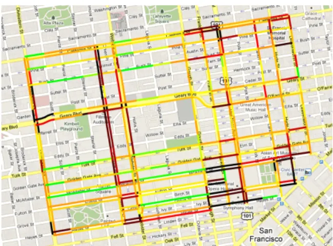
In our case study, we used data from November 25, 2009 through February 27, 2010, focusing on weekdays from 3pm-8pm in the subnetwork of San Francisco depicted in figure 4. This subnetwork contains 322 links (where a link is defined as the road between two signals) and has an
aver-Figure 4. Real-time traffic estimation for a subnetwork of San Francisco studied in this article. The color scale represents the estimated travel time divided by the speed limit travel time. Green is for values close to 1 (travel time is about the same as driving at the speed limit) and black indicates values around 5 (travel time is 5 times slower than driving at the speed limit).
age of 600 observations per half hour time interval. We use 30 minutes (half an hour) as the time interval in the graph-ical model presented in section 3. We assume that the ob-servation probability distribution functionsg(section 3) are independent Gaussians. In general, the choice of a Gaussian distribution restricts the flexibility of the model to capture unique traffic characteristics, but it is also far more tractable to solve in practice. Other “standard” distributions that one could consider are gamma or log-normal, which are more difficult, but possible to use in the framework described in this article. Finding tractable approximation methods for us-ing traffic theory inspired travel time distributions will be the subject of future work.
Our approach requires a training period (section 4) be-fore it can be used to make predictions in real-time. We used data from November 25, 2009 through February 19, 2010 as our training period. We only used Tuesdays, Wednes-days and ThursWednes-days to train our model, which totalled 18 training days (after removing holidays and days with sys-tem malfunctions that prevented data collection). We then tested the model by running it over all Tuesdays, Wednes-days and ThursWednes-days between February 20, 2010 and Febru-ary 27, 2010, which totalled 3 days.
We first learn the traffic density parameters (section 2) for each hour of the day from 3pm to 8pm, where each hour period is assumed to have its own characteristics in terms of the average density on a link. We then run the EM algorithm (section 4) over all the training data, with the assumption that the transition matrix Aand the Gaussian distributions for each link are stationary over the study period. Once the parameters have been learned through the EM algorithm, we use a particle filter to compute the most likely state of each link given real-time data on a test day. Figure 4 shows a map of the subnetwork of San Francisco with each link col-ored according to its level of congestion, defined as the mean travel time divided by a reference free flow travel time. The
Model RMSE (sec) MPE
Graphical (with density) 46 30.1%
Graphical (without density) 50 34.3%
Baseline 63 44.4%
Table 1. Experimental results comparison between the pro-posed graphical model and the baseline model.
free flow travel time is computed as the travel time experi-enced when traveling at the speed limit and accounting for an expected delay (due to traffic signals) under light traffic conditions.
To quantify the validity of our estimates, we compare the actual travel time of an observed path to the estimate ob-tained by summing over the mean travel time for all links of the path. Table 1 shows the root mean squared error (RMSE) and mean percentage error (MPE) of our travel time predic-tions as compared to a baseline approach. The baseline ap-proach computes the average speed for each observation and assigns it to each link along its path. Then all of the speeds on each link are averaged to give a historical average speed for each link. The real-time version of this approach does the same thing and then takes a weighted average between the historical and the real time speed to give a speed estimate for each link of the network, which can be used to estimate travel times. The two versions of the graphical model show the effect of using the density model of section 2.2 to com-pute partial link travel times instead of simply using a travel time proportional to the partial link distance.
These results were computed on the data obtained be-tween February 20 and February 27, 2010. The data was split into two sets, one for computing the real-time traffic estimates and one for computing the error metrics. This was done to ensure an unbiased comparison of the proposed graphical model and the baseline model. Approximately 70% of the data was used for computing the real-time traffic estimates with the other 30% used for computing the error metrics.
6. Conclusion and discussion
In this article, we proposed a new probabilistic mod-eling framework for estimating arterial traffic conditions from sparse probe data. Our initial results suggest that this approach outperforms the baseline approach in predicting short-distance arterial travel times by 36.9% in terms of the root mean squared error metric. We believe that the pro-posed modeling approach provides a fundamental basis for estimating arterial traffic conditions. The key features that our model possesses are:
• Each link has a discrete traffic state that cannot be directly observed.
• Traffic states of nearby links are correlated and evolve over time in a Markov manner (i.e. the future is inde-pendent of the past given the present).
• Expectation maximization provides the right framework for learning the transition and observation model
parame-ters.
There are numerous ways in which our model can be ex-tended to take into account a wider variety of traffic features. These enhancements include:
• Traffic-specific travel time distributions instead of inde-pendent Gaussians.
• Traffic-specific meanings for the discrete states of each link instead of just undersaturated/congested.
• Direct calculation of the E-step and M-step in the EM al-gorithm using the path travel times instead of relying on the travel time allocation step.
• Relate link travel time distributions to route travel time distributions as estimating short-distance travel times are of less interest than longer trips through city network.
Each of the listed items are part of ongoing research and we expect that these enhancements to the basic model will result in a much richer model capable of giving precise route travel time distributions. The ability to reliably esti-mate route travel time distributions will be a valuable tool for commuters, fleets, and public agencies.
Acknowledgement
Special thanks to Timothy Hunter for help with data pre-processing and path inference of the taxi data. Additional thanks to the Mobile Millennium [12] team for their techni-cal support.
We are grateful to the Cabspotting program [1] and the Stamen design team1 for making their San Francisco taxi feed available to us.
References
[1] Cabspotting.http://www.cabspotting.org. [2] S.J. Agbolosu-Amison, B. Park, and I. Yun. Comparative
evaluation of heuristic optimization methods in urban arte-rial network optimization. InIntelligent Transportation Sys-tems, 2009. ITSC ’09. 12th International IEEE Conference on, pages 1–6, 2009.
[3] X. Ban, R. Herring, P. Hao, and A. Bayen. Delay pattern estimation for signalized intersections using sampled travel times. In Proceedings of the 88th Annual Meeting of the Transportation Research Board, Washington, D.C., January 2009.
[4] P. J. Bickel, C. Chen, J. Kwon, J. Rice, E. Van Zwet, and P. Varaiya. Measuring traffic. Statistical Science, 22(4):581– 597, 2007.
[5] M. Brand. Coupled hidden Markov models for modeling in-teracting processes. Technical report, The Media Lab, Mas-sachusetts Institute of Technology, 1997.
[6] C. Daganzo. The cell transmission model: A dynamic repre-sentation of highway traffic consistent with the hydrodynamic theory.Transportation Research B, 28(4):269–287, 1994. [7] C. de Fabritiis, R. Ragona, and G. Valenti. Traffic estimation
and prediction based on real time floating car data. In Intelli-gent Transportation Systems, 2008. ITSC 2008. 11th Interna-tional IEEE Conference on, pages 197–203, 2008.
1http://stamen.com/clients/cabspotting
[8] C. Furtlehner, J. M. Lasgouttes, and A. De La Fortelle. A belief propagation approach to traffic prediction using probe vehicles. InProc. IEEE 10th Int. Conf. Intel. Trans. Sys, pages 1022–1027, 2007.
[9] B. Hellinga, P. Izadpanah, H. Takada, and L. Fu. Decom-posing travel times measured by probe-based traffic moni-toring systems to individual road segments. Transportation Research Part C: Emerging Technologies, 16(6):768 – 782, 2008.
[10] R. Herring, A. Hofleitner, S. Amin, T. Abou Nasr, A. Abdel Khalek, P. Abbeel, and A. Bayen. Using mobile phones to forecast arterial traffic through statistical learning. In 89th Annual Meeting Transportation Research Board, Washington D.C, 2010.
[11] E. Horvitz, J. Apacible, R. Sarin, and L. Liao. Prediction, expectation, and surprise: Methods, designs, and study of a deployed traffic forecasting service. InTwenty-First Confer-ence on Uncertainty in Artificial IntelligConfer-ence, 2005. [12] The Mobile Millennium Project. http://traffic.
berkeley.edu.
[13] T. Hunter, R. Herring, A. Hofleitner, A. Bayen, and P. Abbeel. Trajectory reconstruction of noisy gps probe vehicles in arte-rial traffic.In progress, 2010.
[14] A. Krause, E. Horvitz, A. Kansal, and F. Zhao. Toward com-munity sensing. InProceedings of ACM/IEEE International Conference on Information Processing in Sensor Networks (IPSN), St. Louis, MO, April 2008.
[15] J. Kwon and K. Murphy. Modeling freeway traffic with cou-pled hmms. Technical report, University of California, Berke-ley, 2000.
[16] M. J. Lighthill and G. B. Whitham. On kinematic waves. II. a theory of traffic flow on long crowded roads. Proceedings of the Royal Society of London. Series A, Mathematical and Physical Sciences, 229(1178):317–345, May 1955.
[17] X. Min, J. Hu, Q. Chen, T. Zhang, and Y. Zhang. Short-term traffic flow forecasting of urban network based on dy-namic STARIMA model. InIntelligent Transportation Sys-tems, 2009. ITSC ’09. 12th International IEEE Conference on, pages 1–6, 2009.
[18] T. Park and S. Lee. A Bayesian approach for estimating link travel time on urban arterial road network. InComputational Science and Its Applications ICCSA 2004, pages 1017–1025. Perugia, Italy, May 2004.
[19] S. Russell and P. Norvig. Artificial Intelligence - A Modern Approach. Prentice-Hall, Inc, Englewood Cliffs, NJ, 1995. [20] A. Skabardonis and N. Geroliminis. Real-Time monitoring
and control on signalized arterials. Journal of Intelligent Transportation Systems, 12(2):64–74, March 2008.
[21] X. Sun, L. Munoz, and R. Horowitz. Mixture Kalman filter based highway congestion mode and vehicle density estima-tor and its application. InProceedings of the 2004 American Control Conference, pages 2098–2103, Boston, MA, 2004. [22] A. Thiagarajan, L. R. Sivalingam, K. LaCurts, S. Toledo,
J. Eriksson, S. Madden, and H. Balakrishnan. VTrack: Accu-rate, Energy-Aware Traffic Delay Estimation Using Mobile Phones. In 7th ACM Conference on Embedded Networked Sensor Systems (SenSys), Berkeley, CA, November 2009. [23] D. Work, S. Blandin, O.-P. Tossavainen, B. Piccoli, and
A. Bayen. A distributed highway velocity model for traffic state reconstruction.In press, Applied Research Mathematics eXpress (ARMX), 2010.