Strategies for the Agro-food Sector

(1)

Strategies for the Agro-food Sector

Franco Rosa

University of Udine, Department DIEA rosa@uniud.it

Abstract

The agro-food sector is receiving a great deal of attention for topics of general interest as the food quality, security and safety, alternative uses of crops in food/feed/fuel, growing concern for GHG (Green House Gas) emission, LCA (Life Cycle Assessment), energy consumption. In the EU policies directed to implement sustainable local agro-food systems, the AFSC (agro-food supply chain) is emerging as the central issue in planning integrated farm-food activities performed in a space-time dimension. In this paper it is presented a methodology of regional planning the AFSC supported by empirical evidences about the region FVG (Friuli Venezia Giulia). The reference product is the Mais a crop largely cultivated in the region. A composite information system is used to simulate the evolution of complex scenarios and predict the consequences of food policies and suggest measures to be introduced in the RDP (Regional Development Plan).The integration of technical and economic disciplines allowed to approach the strategy of regional planning in a broader rural development framework to simulate the achievement of macro-micro targets.

Keywords: planning procedure, regional development plan, multifunctional approach, agri-food supply chain, simulation

1 Introduction

Organization.The interest for the elaboration of the agro-food policies has been growing over the last decades, since the new directions of the EU policy (second pillar) focusing on the sustainable production system, rural development and multi-functionality, have pointed out on the importance of a systemic vision of strategies directed to the implementation of the AFSC. The structural changes in agriculture, the diversification of agriculture, the integration with food/feed/fuel industry, the relevance of climatic changes, energy and LCA, the importance of information, have increased the interest for the management of complex Agro-food complex. (Sexton, 2009). The agro-food sector has evolved from the achievement of scale/scope economies, to the broader strategic positioning approach encompassing the risk management, logistic and marketing control extended all steps of the AFSC. These changes impose to manage the network extended to producers, consumers and actors involved in planning the agro-industrial activities sequentially connected in the chain organizations (Boehlje, 1999). Producers, processors, and seller of food products are growingly involved in any sort of network organizations to redistribute the returns and risks among participating partners (Christopher, 2005). New organization models are needed to achieve a higher level of competitiveness (Murdoch et al, 2000) dictated by a host of technological, regulatory and financial reasons to give quick response to rapid changes in consumer preferences for food quality and diversified uses of feedstock in renewable energy and green chemistry industries.( Hobbs and Young, 2000; Bourlakis and Weightman, 2004). To adequately plan the AFSC it is necessary to

(2)

reformulate the strategies to incorporate issues such as production, and logistics (harvesting and transport), marketing and channels, appropriate organizational models based on vertical coordination and hierarchies, (Menard and Valceschini, 2005), unbiased and symmetric distribution of information among partners, risk sharing along the chain (Epperson and Estes, 1999).

Objectives, targets. The AFSC is the reference model for planning new patterns of rural development and potentially a significant building block for future policies designed to influence their evolution. (Van der Ploeg, 2002). To understand the role of AFSC in the more general contest of rural development, it is needed to come to grips with the empirical richness of emerging alternative food networks, by examining how these are built, shaped, and reproduced over time, space and form, the extent to which they actually achieve in terms of rural development objectives. (Marsden et al, 2000a). A broader approach to the AFSC must conciliate the private interests of agents operating at different chain level with the more general interests of the community for the natural resource conservation, protection of biodiversity, pollution control and energy conservation. All these targets must be embedded in the regional policies enhancing the sustainability of the agro-food sector. (Clancy and Kathryn, 2010).

Specificity. However, the models of supply chain currently applied to manufacturing sector disregard the specificity of local resources for the AFSC, the longer period required for the adjustment of resources and technologies, the significant supply and demand uncertainties caused by different sources of risks. (Lowe and Preckel, 2004).

Model. Beside many AFSC functions have been traditionally modeled independently due to the added complexity of developing and finding solutions the integrated multi-echelon models offer potential cost saving benefits (Thomas and Griffin, 1996). Many works are dedicated to strategic, tactical, and operational modeling with deterministic or stochastic approaches to take account of strategic, tactical and operational targets. (Hoag D, 2010). The underlying reasons are to look at the AFSC planning problem from the perspective of the individual farmers, group of farmers, and food industry operators, facing an increasing complexity of production–distribution and risk generated by a combination of production, processing, marketing events. (Ahumada O., J. R. Villalobos, 2009). Other approaches in agricultural planning include the integrate modeling with crop simulation (Alocilja and Ritchie, 1990), fuzzy programming (Biswas and Pal, 2005) and combination with LP, SP and DP, such as time series analysis (Lien and Hardaker, 2001), decision support systems (Recio et al., 2003) and expert systems (Nevo et al., 1994).

An example of an integrated modeling is the processing a pea-based product with the objective to minimize the overall costs of the production, processing transport and storage activities required to obtain the final product. The problem solved with LP procedure gives the quantity of peas to produce at each growing location, the amount of peas hauled from the production to the processing plants, the amount of products to be processed at each facility and estimation of the product line costs. Apaiah and Hendrix (2005).

This paper is organized as it follows: the first part is dedicated to the revision of current literature about AFSC and regional planning, the second part is dedicated to the analysis of simulation AFSC in a regional planning space, the third part is an empirical application of the Mais AFSC for the region FVG and results obtained from simulations are discussed with reference to the regional policy; the fourth part reports conclusion and prospects of implementation the regional planning in future time horizon .

(3)

2 The regional dimension of the AFSC

For the ongoing concept of AFSC, the region is a territory with many dimensions: physical, institutional, political, economic, functional, logistic, endowed by the administrative-autonomy, to formulate policies dedicated to the growth of local system. The regional development strategy is also entangled with the advantages offered by the dynamic process of integration with neighboring countries and synergies achieved by sharing common physical resources, infrastructures, exchanges, economic collaborations and development of common research projects . (Innes J. E.,1995).

However, the historical concept of region is becoming more undefined since these administrative borders are evolving into aggregation of sub-regions, districts, provinces, departments, metropolitan areas (Hance, Ruhf, and Hunt 2006).

These advantages are accrued by the geographic position of region FVG inside the Alpine and Adriatic Euro-region, rich of natural resources, biodiversity, food traditions; representing opportunities to be exploited with the integration in the enlarged geographic area. In 2001 an important constitutional reform has offered to the Italian regions more political autonomy in regional fiscal policies entangling as well the AFSC.1. (Fabbro and Haselsberger,2009)

Figure 1. The Alpine Adriatic: Milan, Munich, Innsbruck, Udine, Lubjana, Wien, Budapest

For the concern of the AFSC the region is the food area where an historical process of accumulation of agricultural resources and labor skills has determined a concentration of

1

Italy is a hybrid combination of a regionalist and a federalist state (asymmetrically structured). After the last devolution reforms approved in November 2005 the 20 regions of Italy have an extended range of legislative and executive powers, but no full financial autonomy. They have independent regional governments and can approve their own statutes but the exercise of all judicial matters is strictly assigned to the central administration. Some 15 out of 20 regions are constituted as "regions with ordinary statute", while 5 regions have a special statute" (Trentino-South Tyrol, Aosta Valley, Friuli-Venezia Giulia, Sardinia and Sicily).

(4)

image-products obtained from family-farm enterprises, gradually integrated in the agro-food processing industry supported by logistic facilities for storage, seasoning and transport addressed to ameliorate the quality of food products and brands to challenge with consumers’ tastes and preferences. Some of the most popular brands are: Prosciutto San Daniele (Ham), Prosciutto Sauris, (Ham) Formaggio Montasio (Cheese),.Vini del Collio and others. (Rosa & Arfini, 1997). Local institutions and authorities have facilitated the implementation of the AFSC in the district area with the promotion of investments in quality, design, image, and brand with the purpose to enhance the quality perception of these food products. However, the dimension of the AFSC could trespass the regional administrative border since the government authority has imposed to extend the AFSC to neighboring regions to open the participation to a larger number of shareholders, to take advantage of the scale economies, to enlarged the market area and gain competitiveness with the territorial brand-image. (Brasili & Fanfani, 2006). An example is offered by the pigs used for San Daniele ham, collected from ten italian regions, subjected to the statutory rules of the DOP for pig breeding, feeding and delivery, enforced by the Consortium San Daniele and certified by Istituto Nord.Est Qualità. The crucial factors for the regional development of AFSC are: a convenient number of suitable farmland for crop production, local climate conditions, proximity to primary upstream industry with logistic connections main communication streams. Then the agro-food chain is operative at multiple levels and scales, resulting in maximum resilience, minimum import, and proactive in strategies of significant economic and social return extended to a large number of stakeholders of the AFSC. The envisaged strategy will care about: i) collaboration in agro-food policies with regards to quality, recognition of typicality and brand protection, ii) land use conservation and preservation of the soil fertility; iii) protection of the endangered species and favoring the biodiversity; iv) improving the perception of the territory and landscape image related to strategies of territorial marketing and promotion of food quality; v) favoring the integrated agro-industrial poles with logistic platforms for transport and storage perishable food products with intermodal connections; vi) connecting producers, processors and consumers in a more integrated network; vii promoting a multifunctional approach, an application of the rural development philosophy. (Wallis 2002).

The self-reliance is obtained by supplying as much of the foods in a region that is physically possible without losing the original quality of the resource base. This means that the intensification of production is a compromise between the maintenance of the soil fertility and the intensification of the production requested by the growing demands of the consumers and food industry that recognize the quality of food products. Decisions made at different levels of the chain must be coordinated in order to achieve these objectives at minimum costs. (Christopher M.,2005).

Production requires to determine the quantity of land planning, timing of operations: plowing, sowing, fertilization, irrigation; determination of resources required for crop growing. The harvesting operations require decisions about the time of crop collection, equipment scheduling, labor use, and transport equipment. The storage operation, includes the inventory control of the agro-foods and conditioning required when the products are stored for seasoning before their distribution. (Beamon, 1998). Storage-related decisions also need to plan the amount to be stored and sold in each period and how to position the inventory along the supply chain. These decisions also require to schedule the hauling from farm to concentration points (stockpiling) and delivery to processing plants. Finally, the distribution function requires to haul the product down through the supply chain to the final delivery. The decisions

(5)

associated with distribution require to face also the logistic of delivery with intermodal transportation mode, route network and shipping schedule. (Fleischmann et al.,2005).

Sustainable production system requires to reduce the energy consumption, waste and hauling distances. Many authors have showed the weakness of local production systems that use more energy and produce higher quantity of GHG because the tractors and trucks of smaller in size, require more trips to haul the crop to CP. Important efficiencies may be gained by aggregating sufficient volumes of supply, and back-hauling. (Pirog, Van Pelt, Enshayan, and Cook 2001). Land resources. Until a recent past the food security was achieved in FVG for the relatively abundance of land compared to population and favorable climatic conditions. (Danuso and others, 2010). This situation has evolved critically in recent times since new uses of land in multipurpose agricultural crops for food, feed, fuel or green chemistry production and consumption for infrastructure, urban, industrial uses are starting to erode a consistent quota of the agricultural land. (Rosa and others, 2010). Planning alternative food strategies means to allocate these resources in sustainable production systems at acceptable scale and intensification to avoid that food supply in the future could be jeopardized. (Fiorese, 2010) Industrial and market facilities. A regional AFSC network is comprised of multiple marketing options for farms of all sizes that include local markets and intermediaries, assuring transactions thereby providing farmers with more market opportunities using alternative channels of the supply chain. In emphasizing the importance of new AFSC solutions some authors have emphasize the potential benefits of ‘short food supply chains’ that ‘short circuit’ long and complex industrial chains. (Marsden, and others, 2000).

These dimensions of AFSC are the key elements for an effective regional food system, and the economic development should strive to support new business relationships based on fairness and transparency throughout the supply chain referred to value chains or values-based food supply chains. The underlying reason for this approach is to look at the AFSC planning from the perspective of group of farmers. The profile of these typical players is the changing model of farm management from family based, small-scale and independent firms to one in which larger firms are more tightly aligned across the production and distribution value chain (Boehlje, 2003).

Regional agricultural policy. The directions of the regional agricultural policy are contained in the RDP (Regional Development Plan) who reports in the axis and measures the intervention and financial provision for the use of agricultural resources (food, feedstock, fuel). The RDP 2007-2013) contains new incentives dedicated to the agro-energy in compliance with the National Strategic Program elaborated under the guidelines of the European Community. Subsidized measures are dedicated primarily to promote the diversification of activities in primary sector developed under the chain scheme. The RDPs supports the development of the agro-energies, to pursue the objectives of diversification and accomplish with the Kyoto Protocol to limit the emission of GHG. The RDPs also includes financial provisions for encourage business investments in AFuelSC (measure 121 "Farm modernization), as well as measures helping companies to invest in plant to convert biomass into energy (measure 123) to add value to agricultural and forestry products. However, the small dimensions of farm size represent a limit to the development of agro-energy programs. Incentives for the development of agro-energy infrastructures areas are contained in measure 321 of the RDPs, dedicated to "Basic services for the economy and rural population". Incentives have also been designed to support the facilities for the production of biogas from animal waste, although more investments are dedicated to biomass from agriculture or forestry to be converted into energy products. In total the region has invested 13 million euros approximately that are additional resources invested in these programs for the period 2007-13.

(6)

3 The AFSC- analysis and simulation

The agricultural territory of the region FVG is extended over 224521 Ha, the land dedicated to annual cereal and oleaginous crops occupies approximately 170 thousand Ha. A previous analysis is performed with the aim to split the regional area in sub-areas with homogeneous climatic conditions. In tab. 1 it is reported the structure of Agriculture in FVG region: 24 thousand farms manage approximately one million parcels, covering a surface of 225 thousand Ha, with an average of 9,43 Ha per farm that is above the national average. Most of the agriculture is concentrated in larger farms: the 56,3 % of the cultivated area is owned by 10% of farmers.

Table 1. Number of farms and surface classified by size in region FVG

Source ISTAT

The regional planning simulation uses information generated by GIS techniques giving reliable pictures of the soil use; these data combined with the traditional statistical sources (ISTAT, INEA, ISMEA). The GIS is used to assess the land use and crop yield, while the data about climate, soil and terrain features are used for the appropriate agro-ecological simulations that represent the core of this analysis. (Fiorese e Guariglio, 2010).

The geographic borders of the basin is defined using a raster spatial analysis simulating a biomass supply distributed across the region with location of biomass production, location of concentration points (that are stockpiling centers similar to country elevators in USA) pointing out the cross borders of the supply basin corresponding to the raster pixels with maximum delivery cost. These collection points are localized in proximity of urban areas or close to some large agricultural areas, nearby the main or secondary road system; and their function is to store conserve and concentrate the agricultural crops for the next processing step. The CP are connected to the Pl with provincial, state and highway. The first part of the analysis is dedicated to the location/allocation problem by finding the shortest distance from parcel to the corresponding CP and from CP to Pl. The crop delivery from CP to one of the processing plants will account of the different distances of the two processing plants. It is assumed the two plants have the same size, industrial characteristics and use similar technologies but they are located at different distances from CP, then the solution based on the minimization of transport cost could privilege the plant situated at minimum distance from the nearest CP. The convenience must be evaluated with the incentives included in the contracts and bargained between farmers and processors. Constraints are applied to the land use to maintain a diversification of agriculture appropriate to the needs of the region. The area invested in crop measured in Ha and costs (including growing, transport, storage and processing crops measured in € are the decision variables used for planning the AFSC and to evaluate the convenience to produce crops over the chain.

The simulation regards the estimation of the potential biomass supply available under given conditions by using integrated database of the farm structure and crop production. A complete set of information regarding the biomass (cultivation, transport, processing, emissions, energy consumption, etc.) is computed. Two processing plants are available in the region for processing the crop delivered. Their size is already predetermined: The plants named CD

variable < 1 1 - 2 2 - 5 5 - 10 10 - 20 20 - 50 > 50 Total number farms 2817 4151 7829 4002 2671 1732 617 23819 % total 11.83 17.43 32.87 16.80 11.21 7.27 2.59 100.00 agricultural land 1696 5845 25111 28125 37365 50973 75406 224521 % total 0.76 2.60 11.18 12.53 16.64 22.70 33.59 100.00 land/farm 0.60 1.41 3.21 7.03 13.99 29.43 122.21 9.43

(7)

(Cereal Docks) and SG (San Giorgio) have approximately the same operative dimensions that are consistently bigger than the actual regional supply available. To avoid to exploit only a limited processing capacity of the plant that would have serious consequences for the costs, different types of cereals and oleaginous crops are processed allowing to exploit the scope economies while the intermodal facilities allow to procure feedstock from different locations enlarging the supply basin to exploit scale economies. Data for the simulation are collected from a variety of sources and combined to build the geographic information system. Each set of homogeneous data represent a layer of information:

Layer 1 - Network composed by of 18 thousand farms and 200 thousand parcels2

Layer 2 - Network composed by of 143 climatic sub-areas defined with meteo stations; Layer 3 - Network composed by 53 stockpiling locations (collection points)

Layer 4 - Network composed by the regional road network with nodes, intersections; Layer5 - Network composed by 2 processing plants

The layers of geographic information, spatial, climatic, soil features, crops, road, connection and other data are combined with mathematical algorithms and query to visualize the results in different formats: graphic and thematic maps, tables, and others. The layer combination, used known earth coordinates (like latitude and longitude) to make sure each layer lines up correctly with the others.

For the all crop location are calculated the different costs categories: i) production costs (budgets of crop production costs using three technologies: low, medium, high input); ii) collection and transport costs of the biomass hauled from the production parcel to the CP and from CP to Pl; iii) processing and delivery costs.

The combination of these data requires to satisfy the following conditions:- unambiguous metadata about geo-information resources;- consistent imaging i.e. the same cartographic representation (colors, line width, symbols ) for 'things' (objects) on the map that were the same;- integrated query and selection possibilities and transparency in case of spatial and thematic analysis of the geo-information content. A second output is given by statistical data about land investment and NR share among the shareholder of the AFSC.

4 The analysis: planning the Mais-AFSC in the region Friuli V.G

Mais is the most important cereal crop in the FVG region; the total arable land is extended to 224521 Ha, however, the surface dedicated to cereal crops is approximately 117339 Ha, the surface used for Mais was in 2008 approximately 85 thousand Ha and declined to 73 thousand Ha in 2009 due to the market crisis. (Rosa, Vasciaveo, 2010). To assess the suitable land for a specific crops, the following spatial data are gathered from digitized regional cartography: Moland with pedological (1:250,000) and phyto-climatic layers (1:500,000) and land use cartographies of ERSA (1:25,000).

Suitable area for crops will satisfy the following parameters: • altitude above sea level: below than 150 m;

• maximum terrain slope: less than 10%;

• soil containing rocks, gravels, pebbles less than 5 centimeter size ;

2 _{layer of production units (provided by Insiel) ): inventory of farms producing crops and}

parcels (updated to 2006) described with morphological and pedologic soil features,

administrative borders, and % of area dedicated to a specific crop. Five layers are used for the simulation about biomass productivity, transport cost , energy consumption and emissions

(8)

• thin upper layer: not deep enough for root development; • soil with pH comprised between 5.0 and 7.5;

• average annual rainfall and temperature of climate areas defined with by the meteo stations;

• protected natural areas, permanent prairies and public property areas are excluded.

Land suitable for crops accounts for a portion of the total land available: the land dedicated to cereals is the 52% of the total; area of industrial crops is 13,4%; horticulture represents the 0,5% and perennial crops the 11,2%.

Table 2. The agricultural land in FVG region (2008)

Product Surface (Ha) %

Annual crops of which 172396,58 76,80

Cereals 117339,30 52,30

Industrial crops 30162,36 13,40

Horticulture and potatoes 1182,19 0,50

Forage crop 14214,07 6,30

Other crops 79,16 0,00

Set aside 9419,51 4,20

Of which Public property 204,57 0,10

Perennial crops 25243,41 11,20

Source: Rica-Inea, L’agricoltura del Friuli Venezia Giulia

For the purpose of this study the crop selected is mais processed in ethanol along the chain; the EU policy subsidizing the renewable energy has increased the interest of farmers for this crop; therefore the regional planning target is the mais surface to be cultivated for ethanol. By the way, other factors are influencing the opportunity cost of crop allocation; in fact the transport costs represents only a small % of the total cost and the cost hauling gap could be compensated by better commitment in bargaining the conditions of delivery, payment and risk sharing between farmers and processor.

5 The simulation of the AFSC

The Mais AFSC is described as a geographically-explicit crop resource allocation and infrastructural network model integrated with techno-economic models to yield a spatial distribution of resource across the region for an optimal network configuration of the supply chain. This analysis has four main components: 1) geographically-explicit crop resource assessments, 2) engineering/economic models of the conversion technologies, 3) models for multi-modal transportation of crop and final products based on existing transportation networks, and 4) supply chain optimization model.

The simulation assumes the explicit spatial distributions of biomass supply, competition among technologies for resources, competition among plants for processing in finding the best design for the biofuel supply chains..(Fiorese, 2010).

(9)

The cost categories are listed below: i) Farm: production costs;

ii) CP: crop concentration: include conditioning, storage, drying, loading/unloading operations;

iii) Pl level: processing costs for transforming crop in final product and delivery to pump; iv) Transport cost: hauling the crop from parcel to CP and from CP to processing plant. However, the costs categories deserving more attention are production and transport for which is given a short description.

5.1 Production costs

The cost analysis used to evaluate a full range of costs incurred in production, including capital cost, operations costs for fertilizer herbicide, irrigation, energy costs, property and income taxes, insurance premiums. Variable cost categories for owned machinery are defined as fuel consumption, repairs and maintenance, and seasonal labor. Other variable cost categories are referred to the purchase of operating inputs, such as fertilizer and pesticides, hauling the crop to a storage or handling facility, and hiring custom work. The fixed costs are for the ownership costs due to capital assets as the land and machinery or fixed labor. The capital need to be estimated on an annual basis to properly allocate the original investment capital to one production period (i.e. one year). One type of ownership cost is the depreciation of a machine during the year and the interest that is the opportunity cost for the capital invested in a durable machine. Technically, these two ownership costs are often categorized as noncash fixed costs because their values do not depend on the level of production. The main cost categories are variable and fixed costs, direct and overhead costs; these costs are transformed into a unique variable cost category by assuming the all operation inherent the Mais cultivation are

performed by an external custom company providing all required farming services. In the following table is reported the list of operations with consumption of factors inherent to a technology used in simulation.

(10)

Table 3.List of farm operation for mais production (technology 1) 3

-

Source – Simulation of Danuso CSS

5.2 Transport costs

Haulage costs are calculated on a total weight only the moisture content differentiate the dry crop transport cost. The optimization process consists in finding the shortest distance between parcel i and collection point j and from collection point j to processing plant m; the two costs are summed together. The transport costs are determined in function of the distance between the parcels and collection points, and from CP to Pl using the available comprehensive transportation networks. The transportation network includes all types of roads with nodes and intersections and is built to enable the calculation of both time and cost of travel between two locations at minimum distance. Thus, each segment of the network is assigned with a mode and speed of travel. Data from a variety of sources are compiled to build the geographic and cost components of the transport network. The costs of biomass and fuel transport by truck, fitted to a linear model are drawn from several sources (Perlack and others, 2003),loading and unloading cost are also included. The intra-county transportation cost is calculated using the average distance from the centroid of any parcel in the region to the collection point and from CP to Pl. This geometric measure uses the perimeter of the parcel to estimate average travel distance.(Parker and others, 2010) and travelling speediness is 15 Km/h for tractors and 60 Km/h for trucks. These data are incorporated into a geo-database in the ArcGIS software

3

Gasoline energy consumption in Mj/ha for farming operations and hauling (diesel emission factors per MJ: 74 gCO2, 0.04 gN2O, 0.028 gCH4, Sinanet, 2008; electricity

Corn: Production technique

Day Operation Time of Labour (h/Ha) Fuel Consumption (Kg/Ha) Energy Consumption (Mj/Ha) 102 Plowing 1,9 43 1806 131 MinFert (N75) 0,1 5 210 132 Planting 1,1 4 168 135 Herbicide (glif2.5) 0,2 1 42 158 MinFert (N75) 0,1 5 210 176 Irrigation (35mm) 6,5 1 42 181 Irrigation (25mm) 191 Irrigation (35mm) 200 Irrigation (40mm) 256 Irrigation (35mm) 311 Harvest 0,3 16 672 Total

(11)

environment. Once the network it is built the Network Analyst extension is used to create an origin-destination cost matrix from all source origins to all potential biorefinery locations. 6 The economic modelling

The simulation will be performed with computation of the costs at production, concentration and processing and transport cost from parcel to CP and from CP to Pl. Production costs are calculated with ERSA and RICA-INEA data and calibrated according with specific local agronomic, climatic conditions and technology used. (Danuso, 2007).

The location of CP and Pl for delivery and processing operation is predetermined since these structures are already operatives.

The performance evaluation of the AFSC uses the farm gate net revenue (NR) total and per capita that is the difference between the gross revenue of the final ethanol minus the all chain relevant costs categories. The farm-gate net revenue is computed by hypothesizing a cooperative solution in which the farmers are directly involved in the chain operations and receive for the crop the price of ethanol minus the sum of the chain costs. The difference with the revenue of an independent partnership may be relevant and depends on procedures to determine the distribution of the chain profits and risk evaluation.

The allocation of farmer’s crop to processing plant is solved with a simulation algorithm based on the minimization of marginal costs determined at the two processing plants that are equally accessible to producers. This problem is presented in the next F.O. equation.

1 - F.O Max m ∑i ∑j ∑k ∑m uk*ck*xijkm*pk –uk*xijkm* cgik –uk*xijkm* ctc*dij - uk*xijkm* ctm djm - uk*xijkm*cpj - uk*xijkm* cpm – uk ck*xijkm*ce*dmn

s.t.

xijkm <= bk

the meaning of the symbols are the following: i = parcel; j = CP; k = crop; m = processing plant

xijkm is the variables representing the size of the parcel i measured in hectare (ha), cultivated with crop k; delivered to CP j and to processing plant m;

uk is the annual yield of the k.th crop, in dry ton/ha. The crop yields are simulated using soil-climate models elaborated with the data of 13 regional meteo stations producing 140 climatic areas (Danuso, 2010);

uk*xijkm is the production of crop k.th obtained from parcel i.th, hauled from farm i.th (i = 1..18000), to collection point j.th (j = 1..53), and from collection point j.th to processing plants m.th (m = 1..2, see fig. 2);

ck is the conversion coefficient of agricultural crop into final processed product; pk is the final price of processed crop k;

cgik is the annual unit cost, in €/ ton, for growing crop k, in parcel i using a technology g; The production costs depend on type of crop, parcel (quality, position, form), climate, technology used;

ctc is the road transportation cost by tractor in €/dry ton/km for hauling one ton of crop from parcel i to CP j, including harvest, loading/unloading. return trip;

ctm is the transport cost by truck in €/dry ton/km for hauling one unit of crop from CPj to Plm; ce is the unit cost for transport liquid ethanol to the pump

cpj is the conditioning cost of the collection point j;

cpm is the cost of processing plant m; it is assumed the two plants are equal in size and technology so the scale economies are not considered in the optimization.

(12)

Cdm is the transport cost from plant m to pump n dij for j = 1..53 is the distance from parcel i to CP j;

djm is the distance from collection plant j to processing plant m;

dmn is the distance from processing plant to pump (for simplicity the pump is one so n = 1) The crop produced in each parcel is hauled to the stockpiling location (CP) following the Dijkstra’s shortest path algorithm; then a second hauling from CP to Pl is also determined in the same way.

7 Simulation of the corn supply and net revenue distribution

The surface invested in Mais crop in region FVG was 85 thosand Ha in 2008 and declined to 73 thousand Ha in 2009. The two processing plants respectively: Oil plant San Giorgio located in San Giorgio Nogaro and Cereal Docks located in Camisano Vicentino are selected as suitable location for farmers to deliver their crops. The distances of the farms from the two plants are considerably different: the average distance from San Giorgio is estimated to be 50 Km while the average distance to Camisano Vicentino is 120 Km, the farmers committed to evaluate the convenience to delivery their crop not exclusively by using the distance criteria but using a trade-off between cost of transport and advantages in bargaining the most favorable contract provisions.

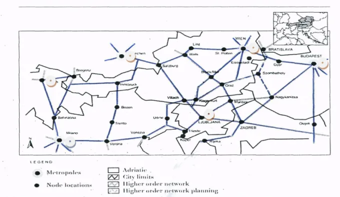
The mais has different uses: silage for feeding cow, feedstock production, fuel; then the maximum of 50% of the total surface dedicated to mais in 2009 is allowed to be used for fuel purpose. Once the total surface is obtained from simulation, the GIS will redistribute across the region. In table 3 it is reported the land used for mais-ethanol production with simulation using the final ethanol price. Tab. 3 and 4 are an exhaustive representation of simulation results obtained for delivery product at the two locations. The maximum surface allowed to be used for Mais cultivation is 36290 Ha that corresponds to the 50% of the total surface invested to mais crop in 2009. By varying the price of ethanol in the range between 1,25 and 1,50 €/l the surface response is comprised in the range between 7436 and 36290 for delivery to SG and in the range between 0 and 36290 for CD.

(13)

Table 3. Mais: determination of surface and net revenue in function of final price and delivery to San Giorgio Plant

Surface quantity of

feedstock fuel produced

chain costs (without accise) chain costs (with accise) Net income (total) Net income (per unit) Price (+ 20% IVA) Price

[ha] [ton] [liter] [Euro] [Euro] [Euro] [Euro / ton] [Euro /liter] [Euro /liter]

7436,22 103194,19 41071286,72 20021229,90 42446152,58 336437,78 0,73 1,25 1,04 25076,23 315618,10 125616005,01 63240880,95 131827219,65 4256785,80 3,04 1,3 1,08 31344,35 377367,34 150192202,34 76856089,50 158861031,98 10105195,73 6,03 1,35 1,13 35492,27 412383,57 164128659,98 85104861,53 174719109,83 16764326,78 9,15 1,4 1,17 36289,77 418420,54 166531374,29 86604801,75 177530932,13 23694478,65 12,74 1,45 1,21 36289,77 418420,54 166531374,29 86604801,75 177530932,13 30633285,83 16,47 1,5 1,25 Surface quantity of

630,83 9947,34 3959041,51 1944033,98 4105670,63 18330,98 0,41 1 0,83 21101,11 285799,32 113748127,65 59032806,53 121139284,28 2087853,98 1,64 1,1 0,92 29995,77 387125,27 154075858,79 81460117,13 165585536,10 7749805,05 4,50 1,2 1 35421,84 440062,24 175144769,66 94005697,95 189634742,33 14700822,30 7,52 1,3 1,08 36289,77 447490,10 178101058,61 95880980,03 193124157,98 22081287,83 11,10 1,4 1,17 36289,77 447490,10 178101058,61 95880980,03 193124157,98 29502165,15 14,83 1,5 1,25 Surface quantity of

0,00 0,00 0,00 0,00 0,00 0,00 0,00 1 0,83 425,18 7107,44 2828760,90 1508327,78 3052831,28 11659,73 0,37 1,1 0,92 16523,69 242191,22 96392104,13 54326924,55 106957013,40 1484103,83 1,38 1,2 1 27313,93 381168,34 151705001,03 87304217,40 170135147,93 6854019,98 4,05 1,3 1,08 34981,53 467282,48 185978424,71 109156976,78 210701196,68 14022733,28 6,75 1,4 1,17 36250,61 479716,61 190927209,06 112543551,45 216789807,60 21869203,73 10,26 1,5 1,25

Low input technology

Medium input technology

(14)

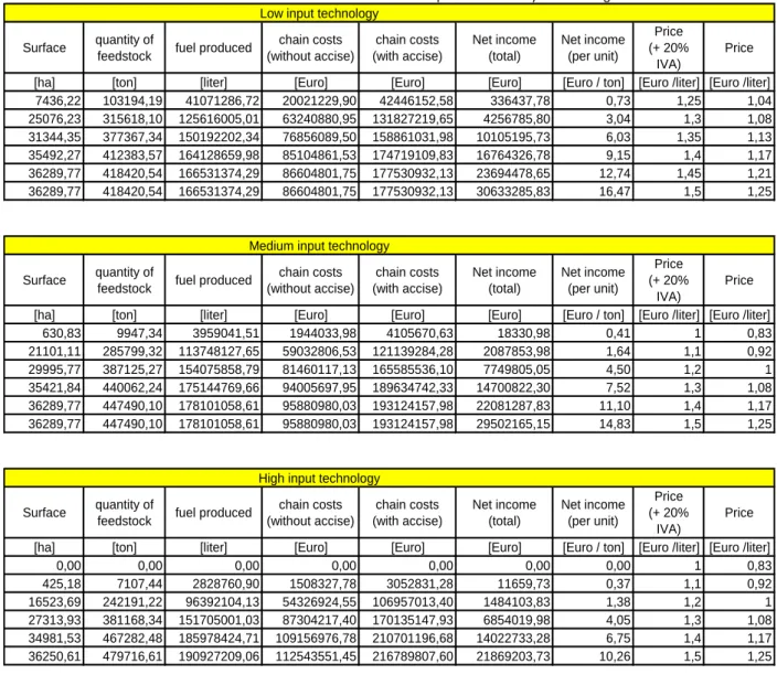
Table 4. Mais: determination of surface and net revenue in function of final price and delivery to Cereal Docks Plant

Surface quantity of

976,73 14474,84 5760984,95 2841571,13 5987069 13957 0,22 1,25 1,04 23027,35 292910,11 116578224,95 60449249,25 124100960 2192117 1,68 1,3 1,08 29818,45 363448,83 144652633,79 76081903,88 155062242 7671971 4,75 1,35 1,13 35378,87 411502,38 163777945,86 87566434,65 176989193 14085077 7,70 1,4 1,17 36250,61 418151,34 166424232,94 89247116,93 180114748 20981200 11,29 1,45 1,21 36289,77 418420,54 166531374,29 89318476,80 180244607 27919611 15,01 1,5 1,25 Surface quantity of

39,60 717,35 285503,13 138496,05 294381 3018 0,95 1,25 1,04 9864,31 140803,36 56039736,60 29446315,43 60044012 665703 1,06 1,3 1,08 26357,55 348071,81 138532579,13 74923826,63 150562615 5286537 3,42 1,35 1,13 34887,83 435164,09 173195308,08 95644174,50 190208813 11852380 6,13 1,4 1,17 36250,61 447180,58 177977871,18 98696946,15 195872864 19183731 9,65 1,45 1,21 36289,77 447490,10 178101058,61 98779725,23 196022903 26603420 13,38 1,5 1,25 Surface quantity of

0,00 0,00 0,00 0,00 0 0 0,00 1,25 1,04 39,60 728,54 289959,68 153678,60 311996 2126 0,66 1,3 1,08 7209,70 110552,35 43999836,03 25040816,55 49064727 435089 0,89 1,35 1,13 24964,19 352915,69 140460443,64 82748605,28 159440007 4430510 2,82 1,4 1,17 32789,42 443866,23 176658758,66 105964177,73 202419860 11042807 5,60 1,45 1,21 35492,04 472451,31 188035619,47 113605677,90 216273126 18771398 8,94 1,5 1,25

Low input technology

Medium input technology

High input technology

Source: archive sossai elaboration/mais26-11-10

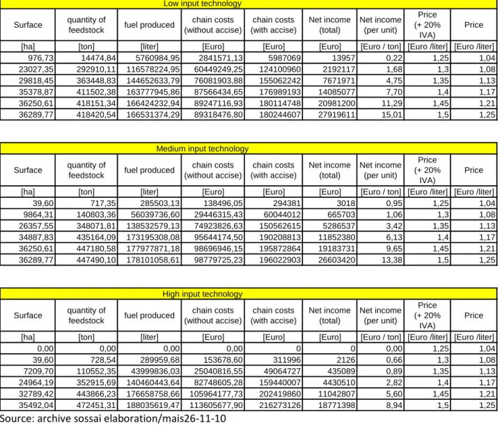
7.1 Surface response to price changes

The surface invested in mais crop is related to the price of the final product over a range of prices predicted by the model. The supply curve has three regions of interest:

i) variation in final crop supply with price, determined by the location of processing plant ii) variable elasticity, higher at the initial stage underlining the higher response of producers to change in final price and positive expectation about profits due to constant corn prices and constant land values for the energy crops that begin to play significant role at these prices. iii) the technology affect the relation yield-cost with consequences for the land investment. As the lower cost resources are exhausted more expensive feedstock and technologies are needed, at the higher prices the supply curve becomes smoother as the response decline The supply curve represents the quantity of final product that could be produced at or below a given cost. The result is derived from the resource assessment, conversion technology models and the deterministic approach to supply chain optimization. It does not account for risks of uncertainty in resource supply, climate events or demand of final product and conversion technology performance. A synthesis of the simulation results obtained for the land investment in function of price of ethanol, location of processing plants and technology used is reported in tab. 5. At the lowest price of 1,25 €/liter of ethanol, the HIT (High input technology) is not economically feasible; with MIT (Medium input technology) there are 40 Ha invested for

(15)

delivery to CD-Pl and 631 Ha invested for delivery SG-Pl; with LIT (Lower input technology), 977 Ha are invested for delivery to CD-Pl and 7436 Ha for delivery to SG-Pl. This gap is rapidly fading out with the increase of ethanol price.

Differences in surface investment at the two Pl by using different technologies:

The difference is rapidly declining with the price increase: with 1,3 €/l the difference in surface using LIT is reduced to 9%, it is still quite large for MIT (114%) and HIT (974);

with price rising to 1,35 the differences are: 5,12% for LIT, 14% for MIT and 129% for HIT; for higher prices the differences become irrelevant.

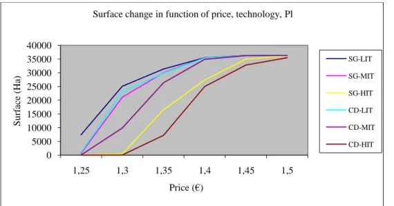
In Fig. 3 it is observed the convergence process that declines rapidly with the price increase.

Table 5. Surface invested in Mais crop in function of ethanol price, technology, delivery plant

Price Delivery to San Giorgio Delivery to Cereal Docks Differences %

LIT MIT HIT LIT MIT HIT LIT MIT HIT

1.25 7436.22 630.83 0.00 976.73 39.60 0.00 661.34 1493.09 n.a 1.3 25076.23 21101.11 425.18 23027.35 9864.31 39.60 8.90 113.91 973.76 1.35 31344.35 29995.77 16523.69 29818.45 26357.55 7209.70 5.12 13.80 129.19 1.4 35492.27 35421.84 27313.93 35378.87 34887.83 24964.19 0.32 1.53 9.41 1.45 36289.77 36289.77 34981.53 36250.61 36250.61 32789.42 0.11 0.11 6.69 1.5 36289.77 36289.77 36250.61 36289.77 36289.77 35492.04 0.00 0.00 2.14

Source: archive sossai elaboration/mais26-11-10

The resources used for Mais production vary over the supply curve (see fig. 3). Many of the resource types become fully exploited over a small range of prices. Market dynamics and diversity not captured in the model would likely increase the range of prices needed for a full exploitation. Note that introduction of sustainability standards, inclusion of indirect land use and other market mediated effects, and other sustainability conditions might significantly alter conclusions regarding corn and energy crop resources.

Figure 3.Surface response to final price change

Source: archive sossai elaboration/mais26-11-10-mais el

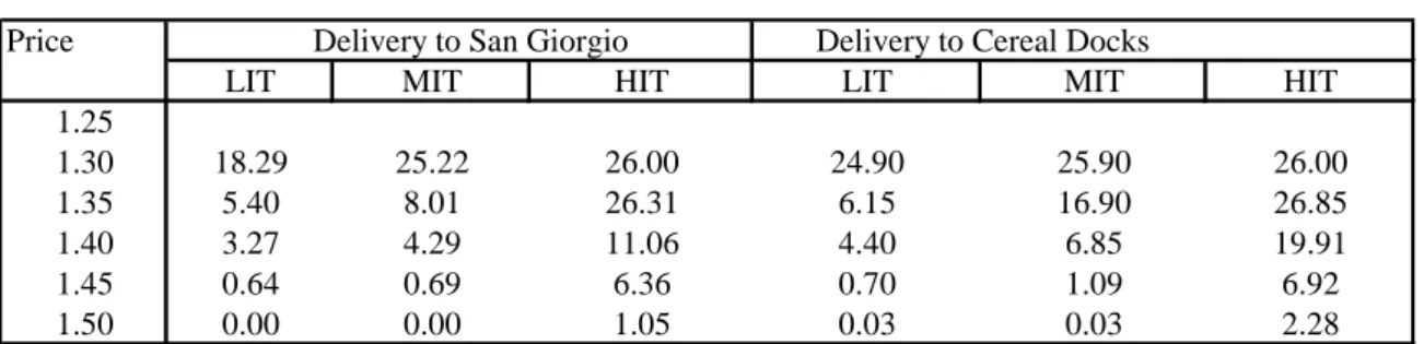
The discrete elasticities shown in tab. 6 confirm the smoothing reaction of surface investment to changes in ethanol price and similar reaction are observed for delivery to SG or CD.

For crop delivery to SG or CD, the rapid decline in elasticity values in response to price change from 1,25 to 1,30 €/l is generalized across the three technologies showing a quick positive response to price change. With the price increase the elasticity values tend to reduce

0 5000 10000 15000 20000 25000 30000 35000 40000 1,25 1,3 1,35 1,4 1,45 1,5 Su rf ace (Ha) Price (€)

Surface change in function of price, technology, Pl

SG-LIT SG-MIT SG-HIT CD-LIT CD-MIT CD-HIT

(16)

consistently and reaction in term of surface cultivated to price changes are almost uniform independently from the technology used. This suggests that the most important factor determining the surface change is the price while technology and location play a marginal role. Then the final price of ethanol must be evaluated carefully by policy makers if they want to favour the AFuelSC.

Table 6. Surface elasticity

Price Delivery to San Giorgio Delivery to Cereal Docks

LIT MIT HIT LIT MIT HIT

1.25 1.30 18.29 25.22 26.00 24.90 25.90 26.00 1.35 5.40 8.01 26.31 6.15 16.90 26.85 1.40 3.27 4.29 11.06 4.40 6.85 19.91 1.45 0.64 0.69 6.36 0.70 1.09 6.92 1.50 0.00 0.00 1.05 0.03 0.03 2.28

The final consideration is for the net revenue calculated with the same variables affecting the surface investment.

Delivery to SG plant: the NRPC (Net revenue per capita) are affected by technology price, and processing location, however the effect of technology and location are inferior compared to price: with prices ranging between 1,25 and 1,50 €/l the NR varied between 0,73 and 14,47 with LIT, between 0,41 and 14,83 with MIT and between 0,22 and 15,01 with HIT.

using LIT is between 0,95 and 13,38 using MIT, between 0 and 8,94 using HIT.

To be noticed the differences of NR between the two plants persist even with higher prices.

Table 7. Net revenue per capita in €/ton

Price Delivery to San Giorgio Delivery to Cereal Docks Difference %

LIT MIT HIT LIT MIT HIT LIT MIT HIT

1.25 0.73 0.41 0.00 0.22 0.95 0.00 239.58 -56.29 n.a 1.3 3.04 1.64 0.37 1.68 1.06 0.66 80.35 54.55 -43.84 1.35 6.03 4.50 1.38 4.75 3.42 0.89 26.86 31.80 55.58 1.4 9.15 7.52 4.05 7.70 6.13 2.82 18.76 22.65 43.27 1.45 12.74 11.10 6.75 11.29 9.65 5.60 12.85 15.01 20.62 1.5 16.47 14.83 10.26 15.01 13.38 8.94 9.71 10.90 14.75

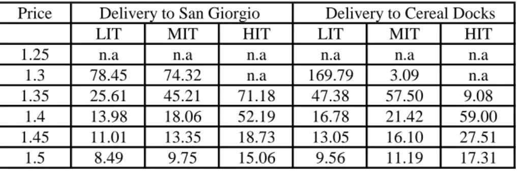
The elasticity values reported in tab. 7 contributes to explain the change of NR in response to price, technologies and location.

For delivery to SG, the NR are growing at decreasing rate in response to price increase, the differences are quite consistent across the technologies and tend to reduce with the price growth.

Delivery to CD: elasticities follow the same pattern as previously explained but the differences among technologies are even bigger.

Non linear response of surface to price changes can be explained by declining yields of less productive land that makes less convenient to invest in Mais.

(17)

Table 8. Elasticity of Net revenue per capita in €/ton

Price Delivery to San Giorgio Delivery to Cereal Docks

LIT MIT HIT LIT MIT HIT

1.25 n.a n.a n.a n.a n.a n.a

1.3 78.45 74.32 n.a 169.79 3.09 n.a 1.35 25.61 45.21 71.18 47.38 57.50 9.08 1.4 13.98 18.06 52.19 16.78 21.42 59.00 1.45 11.01 13.35 18.73 13.05 16.10 27.51 1.5 8.49 9.75 15.06 9.56 11.19 17.31 8 Conclusion

The purpose of this research was to present a methodology of regional planning the AFSC and examine the results in the region FVG (Friuli Venezia Giulia) with the purpose to suggest the guidelines for the RDP. The chain simulation approach was performed with an integrated information system elaborated by GIS and factual information provided by statistical data. The simulation of the effects of different scenarios were transferred to the farmer’s decision about the surface cultivated to Mais and the economic consequences were evaluated in terms of NR. The chain was modeled by using a farm production structure, collection points, and processing plants already existing. The production was modeled by using technical-economic data with three production technologies: low, medium, higher input technologies. The yield was simulated with a combination of technology and climate data generated by the regional meteo stations. The potential surface dedicated to Mais for ethanol was bounded to a maximum of 50% of the total surface cultivated to Mais in 2009 and two destination of feedstock processing were simulated. The parcel represented the elementary unit of simulation and crop transport was optimized using the Dijkstra algorithm. The cooperative model was assumed because ensuring a better NR distribution among farmers. The results suggested the following considerations:

i) the price of the final product was the main factor affecting the farmers’ decisions; the other two factors, technology and distance to Pl counted less. The price signal was more important at the lower level because of the bankrupt risk, the LIT technology was always preferred to other technologies.

ii) farmers didn’t react linearly to price changes: at the lower price level farmers’ response in term of surface investment was much higher and this effect was independent from the type of technology adopted. The non linear response was interpreted as a consequence of the decline in yield as the surface invested in mais increased due to less favorable climatic condition and soil quality.

Suggestion for policy makers were to provide incentives if they wanted reorient the production toward green energy production; the level of incentives must eliminate the opportunity cost offered by using the surface for alternative crops. If they didn’t want to increase the costs of the support policy they could select the most convenient area in term of production or location to Pl;

iii) farmers could profit of these information to decide to allocate their own land, select the appropriate technology and delivery to a preferred plant;

iv) for the purpose of regional planning, the innovation introduced with this procedure consisted in simulate different scenarios by using the final price instead of the farmers price and other variables as land quality, climate effects to observe the profit and risk redistribution across the chain.

(18)

Bibliography

Allen, S.J., Schuster, E.W., (2004).” Controlling the risk for an agricultural harvest”, Manufac-turing & Service Operations Management, 6:225–236.

Alocilja, E.C., Ritchie, J.T., (1990). “The application of SIMOPT2: Rice to evaluate profit and yield-risk in upland-rice production”, Agricultural Systems, 33 (1990): 315–326.

Apaiah, R.K., Hendrix ,E.M.T., (2005).” Design of supply chain network for a pea-based novel protein foods”, Journal of Food Engineering, 70: 383–391.

Aramyan, C., Ondersteijn, O., van Kooten, O., Lansink, A.O., (2006). “Performance indicators in agri-food production chains”, Quantifying the Agri-Food Supply Chain, Springer, The Netherlands (2006) (Chapter 5): 49–66.

Ahumadaa, O., Villalobos, J. R., (2009). “Application of planning models in the agri-food supply chain: a review” European Journal of Operational Research, 196, Issue 1:1-20

Beamon, B.M.,. Ware, T.M., (1998). "A process quality model for the analysis, improvement and control of supply chain systems", Logistics Information Management, 11, 2:105 - 113 Beamon, B.M. Beamon, (1998). “Supply chain design and analysis: Models and methods”,

International Journal of Production Economics, 55:281–294.

Biswas, P., Pal, B.B., (2005).” Application of fuzzy goal programming technique to land use planning in agricultural systems”, Omega, 33: 391–398.

Boehlje, M., Fulton, J., Gray, A., Nilsson, T., (2003). “ Strategic Issues in the Changing

Agricultural Industry”, Purdue University, Department of Agricultural Economics, CES-341. Bourlakis, M.A, Weightman, P.W.H., (2004).” Food Supply Chain Management” Blackwell

Publishing, Oxford, UK.

Brasili ,C., Fanfani, R.,(2006). “Mosaic type of development: the Agri-Food Districts experience in Italy”, Proceeding of the International Association of Agricultural Economists

Conference, Gold Coast, Australia.

Chandra, P., Fisher, M.L., (1994).” Coordination of production and distribution planning”,

European Journal of Operational Research, 72: 503–517.

Clancy, K., Ruhf, K, (2010). “Is Local Enough? Some Arguments for Regional Food Systems”, Choice, 1.st quarter.

Christopher, M., Christopher, D., (2005). “ Logistics and Supply Chain Management”, Prentice Hall, London .

Danuso, F., Rosa, F., Serafino, L., Vidoni, F., (2007). Modelling the agro-energy farm. Proc. Int. Symposium “Farming system design 2007”, September 10-12, 2007 – Catania, Italy, 29-30. Epperson, J.E, Estes, E.A., (1999). “Fruit and vegetable supply-chain management, innovations,

and competitiveness; Cooperative Regional Research Project S-222”, Journal of Food Distribution, 30: 38–43.

Fabbro, S., Haselsberger, B., (2009). “ Spatial Planning Harmonization as a Condition for Trans-National Cooperation: The Case of the Alpine-Adriatic Area” European Planning Studies, 17, 9:1335 – 1356

Fiorese, G., .Guariso, G., (2010). “A GIS-based approach to evaluate biomass potential from energy crops at regional scale” Environmental Modeling & Software, 25: 702-711.

(19)

Fleischmann, B., Meyr, H., Wagner, M., (2005). “Advanced planning, Supply Chain Management and Advanced Planning: Concepts Models, Software and Case Studies”, Springer, Berlin, Germany (Chapter 4).

Hance, A., Ruhf, K., and Hunt, A., (2006).” Regionalist approaches to farm and food policy: a focus on the Northeast”, Northeast Sustainable Agriculture Working Group. Available online: http://www.nefood.org/page/publications-1

Hoag, D., (2010). “Applied risk management in Agriculture”, CRC Press, Atlanta (USA). Innes, J. E., (1995). “Planning Theory’s Emerging Paradigm: Communicative Action and

Interactive Practice”, Journal of Planning Education and Research, 14:183-189. Lazzari, M., Mazzetto, F., (1996). “A PC model for selecting multi-cropping farm machinery

system, Computers and Electronics in Agriculture”, 14: 43–59.

Lien, G., Hardaker, J.B., (2001). “Whole farm planning under uncertainty: Impacts of subsidy scheme and utility function on portfolio choice in Norwegian agriculture”, European

Review of Agricultural Economics, 28: 17–36.

Lowe, T.J., Preckel P.V., (2004). Decision technologies for agribusiness problems: A brief review of selected literature and a call for research, Manufacturing & Service Operations

Management, 6: 201–208.

Marsden, T., Banks, T., and Bristow, G., (2000). “ Food supply chain approaches: exploring their role in rural development”, Sociologia Ruralis 40, 4: 424-438.

Menard, C., (2004). “The Economics of Hybrid Organizations”, Journal of Institutional and theoretical Economics, 160: 345-376.

Menard, C., Valceschini, E., (2005). “New Institutions for Governing the Agro-Food Industry”,

European Review of Agricultural Economics 32, 3: 421-440.

Murdoch, J, Marsden ,T. K., Banks, J., (2000). “Quality, nature, and embeddedness: some theoretical considerations in the context of the food sector'' Economic Geography, 76,2 :107- 125

Nevo, A., Oad, R., Podmore, T., (1994). An integrated expert system for optimal crop planning,

Agricultural Systems, 45: 73–92.

Perlach, R.D., Turhollow A., (2003). “Feedstock cost analysis of corn stower residues for further processing”, Energy, 28: 1395-1403.

Pirog, Rich, Van Pelt, T., Enshayan, K., and Cook, E., (2001). “Food, fuel and freeways: an Iowa perspective on how far food travels, fuel usage and greenhouse gas emissions”. Leopold Center for Sustainable Agriculture.

Recio, B. F., Rubio, F. and Criado J.A, (2003). “A decision support system for farm planning using AgriSupport”, Decision Support Systems, 36, 2: 189–203.

Rosa, F., (2005). “Distretti Agro-alimentari di qualità: fra sviluppo locale e commercio globale: il caso del San Daniele”; contributed paper presented to “ “Il Mosaico Paesaggistico-culturale come volano per il turismo e risorsa”, X° Convegno nazionale Interdisciplinare, Udine.

Rosa, F., Vasciaveo, M., (2010). “Dinamiche dei prezzi agricoli: volatilità, causalità ed efficienza dei mercati agricoli”, contributed paper al XLVII Convegno SIDEA, proceedings,

(20)

Rosa, F., Sossai, E. Vasciaveo, M., 2010. “Planning of the Agrifood supply chain: a case study for the FVG region” European Association of Agricultural Economists, 116th Seminar, October 27-30, 2010, Parma, Italy.

Rosa, F., Arfini ,F., 1997. “Prices and Signals of Quality for Parmigiano and Padano Cheese Markets” in, Schiefer G, R. Helbig edts, “Quality management and Process Improvement for Competitive Advantage in Agriculture and food”, vol. 1: 305-320.

Sexton, R.J., 2009. “Forces shaping the world food market and the role of dominant food retailers”, XVI Convegno SIDEA, Piacenza, Italy: 71-94.

Van der Ploeg, D.J., Long, A., Banks, J., eds, 2002. “Living Country sides: Rural Development Processes in Europe, the State of the Art”, Reed Business Information, Doetinchem Wallis, A.,2002. “The new regionalism: inventing governance structures for the early

Twenty-first Century”. Available online: