The Equity Share in New Issues
and Aggregate Stock Returns
MALCOLM BAKER and JEFFREY WURGLER*
ABSTRACT
The share of equity issues in total new equity and debt issues is a strong predictor of U.S. stock market returns between 1928 and 1997. In particular, firms issue relatively more equity than debt just before periods of low market returns. The equity share in new issues has stable predictive power in both halves of the sample period and after controlling for other known predictors. We do not find support for efficient market explanations of the results. Instead, the fact that the equity share sometimes predicts significantly negative market returns suggests inefficiency and that firms time the market component of their returns when issuing securities.
IN THEIR CLASSIC PROOF of the irrelevance of financing policy, Modigliani and Miller ~1958! implicitly assume market efficiency. If the stock market is inefficient, however, financing policy becomes relevant in obvious ways. When equity prices are too high, existing shareholders benefit by issuing overval-ued equity. When equity prices are too low, issuing debt is preferable.
Consistent with this timing hypothesis, firms issuing equity have poor subsequent performance. Stigler~1964!, Ritter~1991!, Loughran and Ritter ~1995!, and Speiss and Aff leck-Graves~1995!find low average returns after both initial and seasoned offerings.1 These studies focus exclusively on
is-suer returns relative to some benchmark—the first term in the decomposi-tionRi5~Ri2Rb!1Rb. The benchmark is typically the market portfolio or
* Baker is from Harvard University. Wurgler is from the Yale School of Management. We would like to thank John Campbell, Paul Gompers, Jean Helwege, Owen Lamont, Tim Lough-ran, Scott Mayfield, Tom McCraw, Jay Ritter, Bob Shiller, Jeremy Stein, René Stulz, seminar participants at Harvard University, the National Bureau of Economic Research, and the Yale School of Management, and especially Andrei Shleifer for helpful comments. We thank Leslie Jeng, S.P. Kothari, Charles Lee, and CDA Weisenberger for providing data. The issues data series transcribed from theFederal Reserve Bulletin are available on Wurgler’s home page, currently http:00som.yale.edu0;jaw52. This study has been supported by the Division of
Re-search of the Harvard Graduate School of Business Administration.
1See also Friend and Herman ~1964!, Friend and Longstreet ~1967!, Weiss ~1989!, Peavy ~1990!, Jain and Kini ~1994!, Lerner ~1994!, Ikenberry, Lakonishok, and Vermaelen ~1995!, Mikkelson, Partch, and Shah~1997!, Rajan and Servaes ~1996!, Loughran and Ritter~1997!, Loughran and Vijh~1997!, Pagano, Panetta, and Zingales~1998!, Cornett, Mehran, and Tehra-nian~1998!, Teoh, Welch, and Wong~1998a, 1998b!, and Ahn and Shivdasani~1999!for other empirical results that suggest managers time the equity market. However, some authors chal-lenge the idea that firms successfully time the idiosyncratic portion of their returns~Brav and Gompers~1997!, Brav, Geczy and Gompers~2000!, Eckbo, Masulis, and Norli~2000!!.
some other portfolio that moves with the market. But equity issues tend to cluster around market peaks, as shown by Loughran, Ritter, and Rydqvist ~1994! and other studies of “hot issue markets.” This suggests that issuers try to time both their idiosyncratic return and the market return. In this paper, we consider the second possibility.
The empirical financing variable we focus on is the share of equity issues in total equity and debt issues, calculated from data reported in theFederal Re-serve Bulletin. In the typical year between 1927 and 1996, equity issues rep-resent about 21 percent of the value of all new issues. This share increases right after a year of high equity market returns. More interestingly, firms issue rel-atively more equity just before years of low market returns. For example, when the equity share in new issues is in the bottom historical quartile~below 0.14!, the average CRSP value-weighted market return in the next year is 14 per-cent. When the equity share is in the top historical quartile~above 0.27!, the average return in the next year is26 percent. The difference in equal-weighted market returns is even larger, 27 percent versus28 percent.
In terms of sheer univariate predictive power, the equity share in new issues is a stronger predictor of one-year-ahead returns than the dividend-to-price ratio or the book-to-market ratio. It is also statistically significant and of stable magnitude in both the first and second half of the sample. Scaled-price variables, by contrast, do not achieve this level of robustness. Finally, the equity share adds incremental predictive power to the scaled-price variables and other known predictors.
The main question is whether these results have an explanation consis-tent with market efficiency. We consider three explanations. The first and simplest one is that issuing more equity than debt reduces required equity returns through a textbook Modigliani and Miller leverage effect. However, a simple calculation shows that the size of the equity share coefficient is over 20 times too large to be due to this effect alone. Because new issues represent only a small fraction of outstanding capital, they do not inf luence aggregate leverage enough to change expected equity returns.
A second potential explanation is that the equity share is related to future returns through investment. We use a simple representative firm model based on Stein~1996!to understand how investment and financing decisions differ in efficient versus inefficient capital markets. In the efficient market case, if the rational discount rate falls, firms increase investment. If firms follow a pecking-order financing policy, they will also tend to increase the equity share in new issues at the same time they increase investment, giving rise to our main result. However, in the data, aggregate investment is essentially unrelated to subsequent aggregate returns. This conf licts with the efficient market case of the model, which predicts a negative relationship. By con-trast, when mispricing is the primary cause of predictable variation in re-turns, the model illustrates how the equity share may respond to future returns even when investment does not. The empirical analysis in this sec-tion also indicates that the equityshare in new equity and debt issues has somewhat more power to predict market returns than the absolute levelof equity issues.
A third potential explanation is that an unobserved factor such as market risk may simultaneously change both optimal capital structure and required returns in a way that induces a relationship between the equity share and future returns. However, standard theories of optimal capital structure point toward a positive, not negative, relationship between the equity share and future returns. That is, when expected returns go up with risk, the proba-bility of financial distress for a given capital structure rises. And if tax sched-ules are convex, the expected benefit of debt tax shields falls. Given that the costs of leverage increase and the benefits fall, higher risk and returns de-mand more equity, not less. But even if one conjectures the opposite, this channel does not receive empirical support: the predictive power of the eq-uity share does not diminish after controlling for aggregate leverage directly. In sum, we do not find support for any of these efficient market explana-tions for the results. We may have overlooked other potential explanaexplana-tions, but one fact gives pause: the results imply a statistical model of market returns that sometimes predicts significantly negative returns. Because ex-pected returns on the market overall are likely to be positive in any rational model, it is hard to square this with market efficiency. This approach to testing market efficiency has been taken by Fama and Schwert~1977!with the short rate, Fama and French~1988a!with the aggregate dividend yield, and Kothari and Shanken~1997!with the aggregate book-to-market. In con-trast to the results of those studies, we find that the equity share sometimes predicts significantly negative returns even for the value-weighted market. This evidence, and the fact that we cannot find support for any particular efficient market explanation, leads us to conclude that managerial timing of an inefficient equity market is the most credible explanation of our results. Finally, we would like to mention an interesting and related paper by Nelson ~1999!, which, like Loughran et al. ~1994!and this paper, also con-siders the relationship between aggregate financing patterns and aggregate stock returns.2Nelson’s paper can be distinguished from this paper in a few
ways. First, he uses the percentage change in shares outstanding as the financing variable of interest, whereas we use gross new equity issues scaled by gross new equity and debt issues. We believe that the equity share vari-able better isolates timing motives for issuance from pure investment mo-tives and variation in investment opportunities. Nelson’s net series does have the advantage of controlling for repurchases.~We show in Appendix A that controlling for repurchases makes little practical difference to our re-sults, however.!Second, Nelson focuses on a five-year prediction horizon, whereas we focus on a shorter one-year horizon. Third, we go farther than both Nelson and Loughran et al. in ruling out efficient market explanations of the results. The paper proceeds as follows. Section I describes the data on aggregate new issues and other data that we use. Section II presents the main empir-ical results. Section III evaluates efficient market and market timing
expla-2Lamont
~1998!finds that the dividend-payout ratio forecasts high future returns. When dividends are viewed as a source of finance, this predictability is consistent with our findings on the equity share.
nations. Section IV summarizes and discusses some important implications of our results for long-run event studies of managerial actions.
I. Data
For a study of equity market timing, the ideal measure of new finance composition is the share of net new corporate finance raised through public equity issues. The key benefit of the equity share is that it isolates potential timing motives from the level of investment itself. Unfortunately, data are not easily available to construct an ideal measure. Net new finance comes from many sources, including internal finance, new bank debt net of retire-ments, public and private debt issues also net of retireretire-ments, and public and privately placed equity issues net of repurchases. Not all of these data series are available for a significant time period. Our approach is to use a rela-tively unadjusted series of gross new equity and debt issues. We show in Appendix A that various adjustments make little difference to the main re-sults. The data are available at the second author’s home page, currently http:00som.yale.edu0;jaw52.
A. Aggregate Equity and Debt Issues Data, 1927–1996
TheFederal Reserve Bulletinhas reported monthly levels of equity issues ~common and preferred! and debt issues ~public and private! since 1927. Through 1952, theBulletin’s primary source for issues data is the Commer-cial and FinanCommer-cial Chronicle. After 1952, the Bulletinreports data gathered by the Securities and Exchange Commission. Our basic data are the annual totals of equity issues ~common and preferred! and long-term debt issues ~public and private! collected from Bulletinissues between 1927 and 1996. The data series are gross totals of equity and debt issues that do not sub-tract out repurchases or debt retirements. In Appendix A, we show that ad-justing this series by subtracting out repurchases, junk and convertible debt, and utilities issues makes little difference to the main results.
The Federal Reserve Board’s f low of funds provides an alternative source of data on net changes in debt and equity for the economy as a whole. In contrast to the series that we use, these net series subtract repurchases and debt retirements. Unfortunately, there are also disadvantages. The first is that the series include exchange issues and retirements associated with merger activity. Merger activity is often an order of magnitude larger than normal operations finance. As a result, mergers tend to drive the f low of funds se-ries.3A second disadvantage of the f low of funds series is that it does not
begin until 1946. Nonetheless, in Appendix A, we show that the f low of funds data give similar results. All things considered, we lean toward using the unadjusted gross series in the body of the paper.
3We thank Jean Helwege and researchers at the Federal Reserve Board for pointing this out.
B. Hot Markets
The aggregate equity and debt issue series are presented in Figures 1A and 1B. We adjust both to millions of 1995 dollars using the Consumer Price Index. Panel A of Table I reports summary statistics for these series.
Several features of these series are apparent from the plots. First, both series are quite variable. Equity issues are even more variable than debt issues. The standard deviation of the annual growth rate is 96 percent for equity issues and 57 percent for debt issues. Second, hot equity markets, in terms of volume, are apparent.4 Figure 1A shows at least five hot
mar-kets for equity between 1927 and 1996. A peak occurred in 1929, when real new issues surged to $60 billion, a level not reached again until 1983. This level is even more astounding when compared to the size of the stock market. In 1929, new equity represented 11.6 percent of the dollar value of outstanding equity reported by CRSP. By contrast, in 1993, another record year, new issues comprised only 2.3 percent of outstanding equity. Equity issues also peaked in 1971, 1983, and 1986. Third, debt issues rose dra-matically in the 1980s and again in the early 1990s. Real new debt issues increased by a factor of six between 1982 and 1986. Offerings peaked at $630 billion in 1993, about twice the 1986 level. These increases ref lect a variety of factors, including lower inf lation expectations and a growing market for junk bonds.
The issue series are totals that lump together a few different types of issues. For example, the equity issues include not only IPOs and SEOs of operating companies but also issues by closed-end funds. Unfortunately, it is not possible to disaggregate issues by type for the entire period. But bits of data reported in theBulletin and other sources give a sense of how uses of new issues capital vary over time. For example, a large number of closed-end funds were started in 1929. The December 1929Bulletinreports that in the first 10 months of 1929, closed-end company issues represented 42 percent of all domestic corporate security issues. During this period, closed-end funds were priced at large premiums.5The crash sullied the image of these
invest-ment companies for decades after, and they do not represent a large portion of more recent equity issues.
Figure 1A does not reveal the fact that net equity issues were actually negative during most of the 1980s and some of the 1990s, as reported in the Federal Reserve Board’s f low of funds data. This is a consequence of simultaneous increases in repurchase activity and the use of debt to f inance acquisitions ~retiring equity in the process!. Nevertheless, the share of equity in total new issues was also low during this period, and gives a similar impression of financing patterns as the net equity issues series.
4Ibbotson and Jaffe~1975!define hot IPO markets as periods during which initial ~ first-month!IPO returns are particularly high.
5De Long and Shleifer
~1991!discuss closed-end fund issues and discounts around the 1929 crash.
PANEL A. Equity issue volume (e ) in $95M
PANEL B. Debt issue volume (d ) in $95M
PANEL C. The equity share in total new issues (S = e /(e + d ))
Figure 1. Equity and debt issues, 1927–1996.Equity and debt issue volumes are from the Federal Reserve Bulletin. The equity series ~A! includes both common and preferred equity issues. The debt series~B!includes both public and private debt issues. The equity share in total new issues~C!is the fraction of equity issues in total issues. The equity and debt series are converted to 1995 dollars using the Consumer Price Index from Ibbotson Associates~1998!. The data are available at the second author’s web page, currently http:00som.yale.edu0;jaw52.
T able I Summary Statistics Means and standard deviations fo r equity and debt issuance activity , other predictors of equity market returns, and equity market returns. Panel A summar izes equity and debt issue volume from the Federal Reserve Bulletin . The equity issue ser ies ~ e ! includes both common and preferred equity issues. The debt issue ser ies ~ d ! includes both public and pr ivate debt issues. Both ser ies are conver ted to 1995 dollars using the Consumer Pr ice Index from Ibbotson Assoc iates ~ 1998 ! . In Panel B, the T reasury bill return ~ BILL ! and the difference between the long-term government bond and T reasury bill y ields at year end ~ TERM ! are from Ibbotson Assoc iates ~ 1998 ! . The dividend y ields ~ D 0 P ! are calculated separately on the CRSP value-weighted ~ VW ! and equal-weighted ~ EW ! por tf olios. The book-to-market ratio applies to the firms in the Dow Jones Industr ial A verage and is from V alue Line . Panel C summar izes annual returns on the CRSP value-weighted ~ VW ! and equal-weighted ~ EW ! por tf olios. The return ser ies are conver ted to real terms using the Consumer Pr ice Index from Ibbotson Assoc iates ~ 1998 ! . 1927–1996 1927–1961 1962–1996 Mean SD Mean SD Mean SD Panel A: Equity and Debt Issuance Activity Equity issues ~ e ! Level ~ $95M ! 26,780 26,591 10,398 10,937 43,161 27,619 Annual g rowth ~ % ! 29.81 96.45 44.85 126.79 15.20 50.55 Compound g rowth ~ % ! 2.26 — 2 10.58 — 5.62 — Debt issues ~ d ! Level ~ $95M ! 1 17,275 149,341 30,305 13,574 204,244 171,770 Annual g rowth ~ % ! 13.03 57.18 16.63 77.40 9.53 26.43 Compound g rowth ~ % ! 3.74 — 2 3.53 — 5.57 — S 5 e 0 ~ e 1 d ! 0.21 0.1 1 0.22 0.13 0.20 0.09 Panel B: Other Predictors of Equity Market Returns B 0 M 0.68 0.23 0.70 0.21 0.65 0.25 VW D 0 P ~ % ! 4.34 1.25 5.06 1.19 3.63 0.84 EW D 0 P ~ % ! 3.46 1.53 4.55 1.39 2.37 0.62 BILL ~ % ! 3.79 3.28 1.27 1.22 6.32 2.69 TERM ~ % ! 1.50 1.16 1.61 0.95 1.39 1.34 Panel C: Equity Market Returns VW CRSP t 1 1 ~ % ! 8.96 20.56 10.87 24.09 7.04 16.43 EW CRSP t 1 1 ~ % ! 14.26 31.59 17.28 36.73 1 1.24 25.63 VW 2 EW CRSP t1 1 ~ % ! 5.30 16.10 6.41 17.22 4.20 15.07
C. Relatively Hot Markets: The Share of Equity in Total New Issues
We scale equity issues~e!by the sum of equity and debt issues~e1d!. The gross equity and debt issue quantities do not net out repurchases and debt retirements, and the denominator does not include bank debt, internal fi-nance, or finance raised in foreign markets.6Despite these shortcomings, we
believe that the share of equity in gross equity and debt issues is a reason-able ref lection of how firms favor equity or debt over time.7
Figure 1C plots the equity share in new issues from 1927 to 1996, and Panel A of Table I shows some summary statistics. In a typical year, about 21 percent of new issues are equity. The average equity share was about 22 percent between 1927 and 1961 and 20 percent between 1962 and 1996. Due to the high volatility of the equity share in the Depression years, we exam-ine its predictive ability in the full period and separately in the first and second halves of the sample.
Variation in the equity share series comes from both the equity and debt components. The unscaled equity series spikes in 1929, 1971, 1983, 1986, and 1993. Figure 1C shows that the equity market is “relatively hot” in 1929, 1933, 1937, 1946, and 1983. Only two of these years overlap. Some-times the equity market is hot but the debt market is even hotter, and some-times the equity market is cold but the debt market is even colder. More recently, the debt market has been relatively hot—although equity issues have hit record levels and hot IPOs have grabbed headlines, debt issues have grown even faster, keeping the equity share low.
Finally, it is interesting to note that the equity share in new issues was near the middle of its historical range in 1996. The dividend yield and the book-to-market ratio, by contrast, were extraordinarily low in 1996~ Camp-bell and Shiller~1998!!.
D. Other Data
We compare the equity share to other known predictors of market returns. The best-known predictors are the aggregate book-to-market ratio~Kothari and Shanken ~1997!, Pontiff and Schall~1998!!and the aggregate dividend yield~Campbell and Shiller~1988!, Fama and French~1988a!!. In addition, Fama and Schwert~1977!find that the short interest rate is a bearish pre-dictor of nominal market returns, and Keim and Stambaugh~1986!, among others, find that the slope of the yield curve is a bullish predictor.
6Between 1927 and 1950, the Bulletin subdivides equity and debt issues into “new” and “refunding,” based upon the company’s stated purpose for the issue. Refunding finance replaces retired debt or repurchased equity. Between 1927 and 1950, new and total debt issues have a correlation of 0.74, and new and total equity issues have a correlation of 0.99. This provides some comfort in using total issues as a proxy for net issues.
7Hickman~1953!studies the relative frequency of equity to debt offers in the 1900 to 1938 period, and Moore~1983!studies the 1946 to 1970 period.
Panel B of Table I reports summary statistics for these variables. The Dow Jones Industrial Average ~DJIA! book-to-market series is denoted by
B0M.8 The value-weighted dividend yield ~VW D0P! and equal-weighted
dividend yield ~EW D0P! apply to the value-weighted and equal-weighted indices from the Center for Research on Security Prices ~CRSP!. The trea-sury bill return ~BILL! and the difference between the long-term govern-ment bond and Treasury bill yields ~TERM! are from Ibbotson Associates
~1998!.
Panel C of Table I reports summary statistics for the CRSP value-weighted and equal-weighted market indices for various periods. Equal-weighted re-turns have been higher on average, and more volatile, than value-weighted returns.
II. The Equity Share as a Predictor of Stock Market Returns This section describes the predictive power of the equity share for market returns. First, we outline the direction and economic significance of the pre-dictive power. Next, we compare the univariate prepre-dictive power of the div-idend yield, the book-to-market ratio, and the equity share. Finally, we show that the equity share adds new explanatory power to these and other known predictors.
A. Preliminary Analysis
Stock market returns tend to be high following low equity share years and low following high equity share years. Figure 2 illustrates this. We divide the 70 sample years into quartiles according to the prior-year equity share. In the year after bottom-quartile equity share years ~below 0.14!, real value-weighted returns average 14 percent But in the year after top-quartile years ~above 0.27!, real value-weighted returns average 26 percent. As a group, firms lean toward equity just before the market declines.
For value-weighted returns, most of the action appears to be in this high quartile. For equal-weighted returns, however, there is action in both of the extreme quartiles. Equal-weighted market returns average 27 percent fol-lowing bottom-quartile equity share years, versus28 percent following top-quartile equity share years.
8Kothari and Shanken~1997!and Pontiff and Schall~1998!measure annual returns start-ing at the end of March, to be sure that the book values in the book-to-market measure are available before the return period. The book values apply to prior December fiscal year-ends, at the latest. For simplicity, we assume that the book values are known at the beginning of the year. This allows us to use the annual issues data reported in theFederal Reserve Bulletinand the calendar year returns used by most prior authors.
Figures 3A and 3B split the sample into halves. Figure 3A shows the av-erage equal-weighted and value-weighted return for the year before a low equity share year and the five years after, whereas Figure 3B plots the same results around high equity share years. These figures reveal two interesting facts. First, the equity share is related to past returns. Figure 3A shows that firms lean away from equity after a year of low market returns, and Fig-ure 3B shows that firms lean toward equity after a year of high returns. This confirms firm-level findings by Marsh~1982!and aggregate results by Choe, Masulis, and Nanda~1993!. Second, the equity share’s predictive power continues into the second year. Returns are high in each of the two years following a low equity share year and low in each of the two years following a high equity share year.
Table II tabulates the data in Figure 3 more formally. We compare the mean returns in the 10 years surrounding a low equity share year to the mean re-turns in the 10 years surrounding a high equity share year. The table confirms that firms lean toward equity after one year of high returns and before two years of low returns. As suggested by Figure 2, most of these contrasts are even larger when comparing quartile and bottom-quartile years instead of top-half and bottom-top-half years.
Figure 2. Mean equity returns by prior-year equity share in new issues, 1928–1997.
Mean annual real returns on the CRSP value-weighted~light!and equal-weighted ~solid! in-dexes by quartile of the prior-year share of equity issues in total equity and debt issues. Real returns are created using the Consumer Price Index from Ibbotson Associates~1998!.
PANEL A. Mean returns on the VW CRSP (light) and EW (solid) CRSP indexes around low equity share years.
PANEL B. Mean returns on the VW CRSP (light) and EW (solid) CRSP indexes around high equity share years.
Figure 3. Mean past and future equity returns by equity share in new issues, 1928–
1997.Figure 3A plots mean past and future real annual returns on the CRSP value-weighted
~light!and equal-weighted~solid!indexes for below-median equity share years. Figure 3B plots mean returns around above-median equity share years. Real returns are created using the Consumer Price Index from Ibbotson Associates~1998!.
T able II Past and Future Equity Returns around High and Low Equity Share Y ears, 1928–1997 Stock returns are mean annual real returns on the CRSP value-weighted ~ VW ! and equal-weighted ~ EW ! por tf olios. The returns are divided according to whether the year zero share of equity issues in total issues was below or above the median share of 0.204. t -statistics test the hypothesis of no difference between average returns. VW CRSP EW CRSP Y ear Relative Low Share High Share Difference t -Statistic Low Share High Share Difference t -Statistic 2 5 8.66 8.66 2 0.01 @ 0.00 # 12.68 15.62 2.94 @ 0.36 # 2 4 1 1.53 5.33 2 6.21 @ 2 1.21 # 14.70 13.69 2 1.01 @ 2 0.13 # 2 3 9.26 7.91 2 1.36 @ 2 0.27 # 13.48 15.31 1.83 @ 0.23 # 2 2 7.31 9.64 2.34 @ 0.46 # 1 1.19 17.06 5.87 @ 0.75 # 2 1 5.53 12.14 6.61 @ 1.34 # 9.30 19.28 9.97 @ 1.31 # 1 13.74 4.00 2 9.74 @ 2 2.04 # 22.50 5.64 2 16.86 @ 2 2.31 # 2 12.32 4.12 2 8.20 @ 2 1.69 # 21.61 5.91 2 15.70 @ 2 2.09 # 3 7.94 8.89 0.94 @ 0.19 # 12.79 15.53 2.74 @ 0.35 # 4 9.14 8.73 2 0.41 @ 2 0.08 # 14.58 15.28 0.70 @ 0.09 # 5 9.05 10.18 1.13 @ 0.23 # 14.06 17.25 3.19 @ 0.42 #
B. Univariate Regressions
In this subsection we compare the univariate predictive power of the div-idend yield, the book-to-market ratio, and the equity share for equity mar-ket returns. Table III presents OLS regressions of one-year-ahead stock returns ~RE! on these predictors ~X!:
REt5a1bXt211ut. ~1!
The predictor variables are standardized so that the coeff icients are comparable—a one standard deviation increase inXpredictsbpercent higher returns.9
We estimate equation~1!over the full sample period and over the first and second halves. Panel A reports estimates for the full period. The adjustedR2
for the equity share is 0.12 for value-weighted returns and 0.16 for equal-weighted returns. A one standard deviation increase in the equity share~0.11! reduces average value-weighted returns by about 7 percent. For equal-weighted returns, the effect is larger. In the full period, the book-to-market ratio ~B0M! does about as well as the equity share in predicting equal-weighted returns but not nearly as well in predicting value-equal-weighted re-turns. As a consequence,B0M is best at predicting a measure of small stock returns, the difference between the equal-weighted and value-weighted re-turns. The dividend-to-price ratio is marginally significant for both equal-weighted and value-equal-weighted returns but is not as strong as the equity share. In the full sample, the equity share is the best single explanatory variable for both equal-weighted and value-weighted returns.
Panel B and Panel C confirm that each of the variables has some predic-tive power within certain subperiods, with exceptions: the dividend yield ~D0P! does not predict the first half equal-weighted returns, and B0M does not predict the second half value-weighted returns. The coefficients on D0P
andB0M also tend to vary dramatically across the two periods. In contrast, the equity share has roughly the same economic and statistical significance in both periods.
We have also split the sample by prewar and postwar subperiods to ex-amine the robustness of the equity share’s performance in the volatile De-pression years. We find it is statistically significant and of similar magnitude across these subperiods also. For VW returns, the coefficient is 26.70 ~t5 22.70!using 1928 to 1945 returns and28.96 ~t5 22.61! using the 1946 to 1997 returns. For EW returns, the coefficient is 213.21 ~t 5 22.73! using 1928 to 1945 returns and213.06~t5 22.60!using the 1946 to 1997 returns. 9If predictability could ref lect inefficiency, it is inaccurate to state thatXcaptures variation in “expected returns.” One needs to define who is doing the expecting. It certainly would not be the investors holding long positions during a period of predictably low or negative returns. We think it is better to take the more agnostic view thatXref lects in-sample predictability, given the model rather than the potentially misleading phrase, “expected returns.”
T able III Univariate OLS Reg ressions for Predicting One-Y ear -Ahead Market Returns OLS reg ressions of annual real equity market returns on three predictors: REt 5 a 1 bX t 2 1 1 ut where RE denotes real percentage returns on the CRSP value-weighted ~ VW ! or equal-weighted ~ EW ! por tf olio and X var iously denotes the dividend-to-pr ice ratio ~ D 0 P ! , the book-to-market ratio ~ B 0 M ! , o r the equity share in total new equity and debt issues ~ S 5 e 0 ~ e 1 d !! . The dividend-to-pr ice ratio, the book-to-market ratio, and the equity share in new issues are standardized to have zero mean and unit var iance. t -statistics are shown in brackets using heteroskedastic ity robust standard errors. D 0 PB 0 MS bt ~ b ! OR 2 bt ~ b ! OR 2 bt ~ b ! OR 2 Panel A: 1928–1997 Returns VW CRSP 5.01 @ 2.12 # 0.04 4.61 @ 1.79 # 0.04 2 7.42 @ 2 3.86 # 0.12 EW CRSP 5.75 @ 2.04 # 0.02 13.06 @ 2.83 # 0.16 2 13.12 @ 2 3.64 # 0.16 EW 2 VW CRSP 2.87 @ 1.81 # 0.02 8.45 @ 3.37 # 0.26 2 5.70 @ 2 2.69 # 0.1 1 Panel B: 1928–1962 Returns VW CRSP 8.36 @ 2.40 # 0.08 12.24 @ 3.00 # 0.19 2 7.39 @ 2 3.14 # 0.1 1 EW CRSP 6.24 @ 1.08 # 2 0.01 26.64 @ 3.84 # 0.41 2 14.24 @ 2 2.97 # 0.19 EW 2 VW CRSP 0.88 @ 0.32 # 2 0.03 14.40 @ 3.69 # 0.56 2 6.84 @ 2 2.33 # 0.20 Panel C: 1963–1997 Returns VW CRSP 4.02 @ 0.95 # 0.00 2 0.73 @ 2 0.29 # 2 0.03 2 7.82 @ 2 1.99 # 0.1 1 EW CRSP 24.32 @ 2.95 # 0.12 3.56 @ 1.13 # 2 0.01 2 1 1.20 @ 2 1.98 # 0.09 EW 2 VW CRSP 21.48 @ 4.78 # 0.30 4.29 @ 2.90 # 0.07 2 3.38 @ 2 1.13 # 0.00
In Appendix A, we show that netting out repurchases, or making other allowances for junk and convertible debt or utilities issues, is of little con-sequence to the univariate results. The resulting series tend to be highly correlated with our unadjusted equity share series, and the predictive power is essentially the same.
On a statistical point, it has been noted that theD0PandB0M coefficients are subject to an upward small-sample bias.10 Nelson and Kim~1993!show
this in a simple system:
REt5a1bXt211ut, ~2!
Xt5c1dXt211vt. ~3!
In this setup, the bias in estimating the OLS coefficient forbdepends on the contemporaneous covariance between the two residuals, u and v, and the
bias in the OLS estimate ofd ~Stambaugh ~2000!!:
E@bZ 2b#5 suv
sv2 E@dZ 2d#. ~4!
where the hats denote OLS estimates.
For the scaled-price variables, one expects the residuals of equation ~3! to covary negatively with the residuals from equation ~2!. For example, an unusually high return increases the denominator of the scaled-price pre-dictor. In addition, the bias in estimatingdis also negative ~Kendall~1954!!. From equation ~4!, the OLS estimate of b is biased upward for D0P and
B0M. Therefore Table III overstates the economic significance of these predictors.
We do not expect the equity share coefficient to be similarly biased be-cause it is not highly autocorrelated and it is not a scaled-price variable. To verify this, we calculated the empirical correlation for the OLS residuals for equations ~2! and ~3! for each of the three predictor variables. The results are presented in Table IV. For the book-to-market ratio and dividend yield, we replicate the findings of Kothari and Shanken~1997!. There is a signif-icant negative contemporaneous correlation between the residuals ranging from20.7 to20.9. The equity share residuals, by contrast, show little cor-relation. Table IV also reports bias-adjusted estimators based on Kendall’s correction for autocorrelated regressors, as suggested by Kothari and Shan-ken. The scaled-price variables’ bias-adjusted coefficient estimates are 15 percent to 45 percent smaller than their OLS estimates, but the adjustment makes almost no difference for the equity share.
10Kothari and Shanken
C. Multivariate Regressions
In this section we examine the incremental power of the equity share over other predictors of aggregate returns. Table V presents OLS regressions of equity market index returns ~RE! on past returns, the Treasury bill return
Table IV
Correlation of the Residuals for the Univariate Market Regression and the Predictor Autoregression, 1928–1997
OLS regressions of annual real equity market returns and autoregressions for three predictors:
REt5a1bXt211ut
Xt5c1dXt211vt
whereREdenotes real percentage returns on the CRSP value-weighted~VW!or equal-weighted ~EW! portfolio andX variously denotes the dividend-to-price ratio~D0P!, the book-to-market
ratio~B0M!, or the equity share in total new equity and debt issues~S5e0~e1d!!. Panel A
shows OLS estimates ofaandb. Panel B shows estimates ofcandd. Panel C shows estimates of the correlation between the two residuals,uandv, and tests its significance level against a
null hypothesis of zero correlation. In addition, we calculate bias-adjusted estimates ofb fol-lowing Kothari and Shanken ~1997, equation ~4!!. The dividend-to-price ratio, the book-to-market ratio, and the equity share are standardized to have zero mean and unit variance. t-statistics are shown in brackets using heteroskedasticity robust standard errors.
D0P B0M S
VW CRSP EW CRSP VW CRSP EW CRSP VW CRSP EW CRSP Panel A: Market Return OLS regression
Intercepta 8.72 13.96 8.87 14.07 8.93 14.17 @3.65# @3.75# @3.70# @4.08# @3.89# @4.10# Slopeb 5.01 5.75 4.61 13.06 27.42 213.12 @2.12# @2.04# @1.79# @2.83# @23.86# @23.64# O R2 0.04 0.02 0.04 0.16 0.12 0.16
Panel B: Predictor OLS Autoregression
Interceptc 23.20 22.26 20.39 21.07 @20.48# @20.42# @20.05# @20.10# Sloped 0.85 0.91 0.78 0.45 @9.12# @17.44# @7.17# @2.41# O R2 0.68 0.80 0.57 0.19
Panel C: Bias-Adjusted Estimate
ruv 20.70 20.67 20.87 20.78 0.11 0.11 p-value 0.00 0.00 0.00 0.00 0.37 0.36 suv0sv 2 224.46 245.82 226.61 234.43 2.33 3.54 Bias adjustedb 3.71 3.20 3.28 11.35 27.34 213.00 N 70 70 70 70 70 70
~BILL!, the term premium ~TERM!, the dividend yield ~D0P!, the book-to-market ratio ~B0M!, and the equity share ~S!:
REt5a1b1REt211b2BILLt211b3TERMt211b4D0Pt211b5B0Mt21
1b6St211ut. ~5!
Fama and French~1988b!and Poterba and Summers ~1988! find that mar-ket returns have a small negative autocorrelation at one-year horizons, so we include the lagged market return. The last three predictor variables are again standardized to have zero mean and unit variance. We estimate equa-tion~5!over the full sample period and over the first and second halves.
Table V
Multivariate OLS Regressions for Predicting One-Year-Ahead Market Returns
OLS regressions of annual real equity market returns on multiple predictors:
REt5a1b1REt211b2BILLt211b3TERMt211b4D0Pt211b5B0Mt211b6St211ut
whereREdenotes real percentage returns on the CRSP value-weighted~VW!or equal-weighted ~EW!portfolio,BILLdenotes the return on Treasury bills,TERMdenotes the yield premium of long-term government bonds over treasuries,D0Pdenotes the dividend-to-price ratio,B0M
de-notes the book-to-market ratio, andSdenotes the equity share in new issues. The dividend-to-price ratio, the book-to-market ratio, and the equity share are standardized to have zero mean and unit variance.t-statistics are shown in brackets using heteroskedasticity robust standard errors.
1928–1997 Returns 1928–1962 Returns 1963–1997 Returns VW CRSP EW CRSP VW CRSP EW CRSP VW CRSP EW CRSP Intercept 6.95 21.72 14.33 21.71 11.50 19.23 @1.13# @1.68# @0.53# @0.76# @0.78# @1.16# RE 0.05 0.08 0.27 0.20 20.20 20.09 @0.39# @0.82# @1.12# @1.09# @21.01# @20.68# BILL 0.71 20.85 4.96 9.60 0.66 4.20 @0.89# @20.47# @0.75# @1.28# @0.40# @1.46# TERM 20.86 23.66 27.98 210.86 0.15 6.09 @20.41# @20.96# @20.70# @20.84# @0.08# @1.45# D0P 4.26 21.58 24.37 29.17 14.51 63.21 @1.13# @20.27# @20.51# @21.55# @1.43# @2.41# B0M 1.51 13.50 19.59 34.10 27.30 214.30 @0.38# @2.38# @1.99# @6.34# @21.29# @21.47# S 27.88 213.17 28.84 214.34 28.27 213.63 1 @23.97# @23.77# @21.94# @22.21# @22.13# @22.48# O R2 0.12 0.28 0.27 0.51 0.12 0.29 N 70 70 35 35 35 35
Table V shows that, across different sample periods and market return indices, the equity share is the most consistently significant predictive vari-able. For the entire period, the equity share is significant at the one percent level for both value-weighted and equal-weighted returns. Neither the div-idend yield nor the book-to-market ratio is significant for value-weighted returns. The book-to-market ratio’s strong first half performance is enough to make it significant for equal-weighted returns over the full period, but it does not help to predict value-weighted returns. In fact, both the B0M and
D0P coefficients change sign from the first half to the second half. Pontiff and Schall~1998!discuss the erratic predictive ability ofB0Min more detail. There does not appear to be any mean reversion ~conditional on the other variables! at the one-year horizon.11 Finally, the bond market variables we
consider are weak predictors of real returns.12
The equity share is not significantly correlated with either the dividend yield or the book-to-market ratio. Therefore its predictive power is comple-mentary. However, the scaled-price variables are themselves highly corre-lated, as Kothari and Shanken ~1997! show. In our sample the correlation between VW D0P ~EWD0P! and B0M is 0.68 ~0.43! and is statistically sig-nificant. Because book value and dividends are both highly persistent, most of the variation in the scaled-price variables comes from changes in their common denominator.
One implication of this high correlation is that the parameter instability of these coefficients may in part ref lect collinearity. A second implication is that looking at the scaled-price variables separately may understate their combined significance. To evaluate the latter possibility, we perform an
F-test of the hypothesis that D0P and B0M together have no predictive power. For the full sample, we can almost reject this hypothesis at the five percent level for value-weighted returns~p-value50.053!. This hypothesis is more strongly rejected for equal-weighted returns; in the full sample, scaled-price variables do have some joint explanatory power for equal-weighted returns, even after the equity share and other conditioning vari-ables are included.
III. Interpreting the Results: Efficient Market or Market Timing? Unless we agree that rational expected returns are constant, the fact that the equity share predicts returns does not by itself demonstrate inefficiency. In this section we consider three ways in which the equity share in new 11The five-year average equity share does not do well at predicting average returns over the next five years~unreported!. This highlights the fact that the equity share’s predictive power comes at a much shorter horizon than the mean reversion documented in Fama and French
~1988b!and Poterba and Summers~1988!.
12The deviation of the Treasury yield from its six-month moving average produces a stron-ger negative coefficient than that which we report forBILL. Use of this alternative short-term rate indicator does not change the predictive power of the equity share, however.
issues could be negatively related to rationally time-varying returns. Find-ing that none is supported by the data, we turn to the market timFind-ing explanation.
A. Modigliani and Miller Effect
In the framework of Modigliani and Miller~1958!, an increase in leverage causes an increase in the expected return on equity. Because aggregate le-verage tends to increase when the equity share is low, this effect produces a negative relationship between the equity share and future returns, as we found empirically.
However, the empirical equity share coefficient is much too large to be explained by this effect. In particular, it is straightforward to show that the first-order effect of new issues, as measured by the equity share, on expected equity returns is
dE@RE#
dS 5
2aE@RA2RD#
S2 ~6!
where a is the ratio of new equity issues to the aggregate value of equity including the new issues,E@RA2 RD# is the expected excess return of total corporate assets over corporate debt, andSis the equity share in new issues.13
We can use historical averages to measure these quantities and then com-pare the predicted theoretical effect of the equity share with the actual co-efficient in Table III and Table V. From 1927 to 1996, the average ratio of new equity issues to the aggregate market value of equity was 1.7 percent. Over the same period, the average excess large company stock return over corporate debt was approximately 6.5 percent, as reported in Ibbotson As-sociates ~1998!. Because expected equity returns must be higher than ex-pected asset returns, this represents an upper bound for the excess return of assets over debt. Finally, the average equity share in new issues was 0.21. Plugging these values into equation~6!gives a bound of22.5. To compare this with the standardized empirical results, we multiply by 0.11, the stan-dard deviation of the equity share. This yields a predicted theoretical equity share coefficient of20.28, as compared to actual coefficients between27.42 ~from the univariate analysis! and 27.88 ~from the multivariate analysis!. This analysis indicates that the leverage risk effect explains less than one-twentieth of the equity share’s actual effect.
13The first step is to write postissue leverage as a weighted average of the leverage exclud-ing new issues and the leverage of the new issues themselves. The second step is to rewrite the leverage of new issues in terms of the equity share. The third step is to substitute the resulting expression for postissue leverageLinto the Modigliani and Miller arbitrage conditionE@RE#5
E@RA#1L@RA2RD#. The final step is to differentiateE@RE#with respect toS. We ignore the
derivative ofRDwith respect to Sand therefore derive an upper bound impact of the equity
B. Investment
The equity share could be negatively related to rationally time-varying future returns through investment. For example, if the rational discount rate falls, firms will increase investment, and the equity share may increase incidentally if firms follow a pecking-order policy. Myers and Majluf ~1984! show that when managers have information that investors do not have, ex-ternal finance is more costly than inex-ternal finance, and equity is more costly than debt. If in addition firms have a fixed debt capacity, the ratio of equity to external finance will increase with financing requirements, that is, the equity share rises with investment.
This story makes the additional prediction that the level of investment forecasts rational variation in returns. Importantly, as we show using a model of investment and financing based on Stein~1996!, optimal investment need not depend on variation in returns due to mispricing. We develop these theo-retical predictions and then check whether the level of aggregate investment is actually negatively related to subsequent returns. Because it is not, we do not advocate explanation for the equity share’s predictive power based on a link through investment to a time-varying discount rate.
Stein argues that there are three factors that determine the level and composition of securities issues: the value of the investment opportunity itself; the market timing gain ~if any! associated with new issues; and the cost of deviating from optimal capital structure. In a simple reduced form, these factors may be summarized in the following managerial decision prob-lem for a representative firm:
max
S,I f~I!2~11E@RA#!I2dSI2i~SI!2z~~S2SO!I!. ~7! The manager chooses the equity share in new issues,S, and the level of total equity and debt issues,I. The product SI therefore denotes the level of eq-uity issues~e elsewhere in the paper!, and I2 SI denotes the level of debt issues~d elsewhere!.
The project’s expected payoff isf~{!, which is increasing and concave. The rational expected return on financial assets isE@RA#, which may vary from period to period. The third and fourth terms represent the market timing gains associated with equity issues.dis the irrational component of expected equity returns and also may vary from period to period. ~When equity is overpriced, d is negative.! The announcement effect associated with equity issues and repurchases,i~{!, is represented by a cost function that is U-shaped around zero. Thus, the bigger is the announced equity issue or repurchase, the more suspicious new shareholders are that they are being exploited, and the more they revalue the firm to reduce the scope for market timing. The cost of deviating from optimal capital structure is given by the final term,
cap-ital structure would be maintained if the manager set the equity share atSO. Above SO, agency costs and lost tax shields exceed reductions in expected financial distress costs. BelowSO, the opposite is true.14
The comparative statics of this program show how investment and the equity share respond to the parameters E@RA#and d. Note this model does not explain how or why the market may be mispriced in the f irst place. Instead, it guides a search for comparative statics predictions that may help to discriminate between efficient market and inefficient market explanations for our main results, a relationship between financing activity and returns.
We would ideally like to compute comparative statics with respect toE@RE# ~the rational expected return on equity! and d because full-information ex-pected equity returns areE@RE#1d. In a rational model of returns, there is a direct link between E@RE# and E@RA# through a Modigliani and Miller relationship. Of course, equation ~6! shows thatE@RE#also depends on the change in leverage induced by new issues, but we just found the effect to be negligible.
In Panel A of Table VI, we report comparative statics results for the effi-cient markets case: E@RA# varies over time, but d is always zero. The cal-culations are in Appendix B. The comparative statics turn out to be sensitive to whether information costs,i~{!, or suboptimal leverage costs, z~{!, domi-nate, so we report results for both cases. In the first case, information costs are assumed to dominate. When required returns E@RA# increase, for in-stance, investment falls. Because the announcement effect is increasing in the dollar value of equity issues ~SI!, a lower level of investment allows a larger share of equity issues. Thus,S rises withE@RA#.
In the second case, the cost of deviating from optimal leverage is assumed to dominate. Because there is an announcement effect, the equity share will always be below the share that keeps leverage at the optimum,SO. As before, when required returns increase, investment falls. Now, because the cost of deviating from optimal leverage is increasing in the dollar value of equity issues, lower investment allows an even smaller equity share, so Sfalls.
The second case demonstrates how, in some circumstances, a high equity share could forecast low equity returns even in the absence of a timing mo-tive. But an unambiguous prediction of all efficient markets cases is that there should be a strong negative relationship between investment and sub-sequent returns. This is true regardless of the structure of information and suboptimal leverage costs.
In Panel B, we summarize predictions of the polar inefficient markets case:E@RA#is constant, butdvaries. The results are quite different from the efficient markets case. If information costs dominate, mispricing has little 14See Stein’s paper~1996!for more discussion of the structure of equation~7!. Despite the simplifications apparent in this stylized setup, some issues still have to be ignored to keep the analysis tractable. For one, the model assumes no internal finance is available; investment equals the total raised through new issues. The model also ignores the option to delay investment.
effect on investment. Investment is primarily determined by E@RA#, which is assumed roughly constant, so the upshot is that one observes no correla-tion between investment and subsequent equity returns. And now timing motives are apparent: the equity share rises when equity is overvalued, that is, whend is negative.
If suboptimal leverage costs dominate, on the other hand, investment and financing are not separable. In the absence of mispricing, the equity share would be set at SO. But maintaining this ratio imposes costs and benefits throughd. The negative relationship between investment and returns reap-pears, but the relationship between the equity share and returns can go either way, depending on the degree of mispricing.
The takeaway is that investment should be strongly negatively related to rational, predictable variation in returns but need not be related to returns driven by mispricing. To evaluate the empirical link between investment and subsequent returns, we gather net nonresidential fixed capital stock
Table VI
Comparative Statics of an Investment and Financing Model
This table summarizes comparative statics predictions made by a representative-firm security issue model based on Stein~1996!:
max
S,I f~I!2~11E@RA# !I2dSI2i~SI!2z~~S2SO!I!.
The manager chooses the equity share~S5e0e1d!and the level of investment~I5e1d!to
maximize an objective that depends on the project’s expected payoff~f~{!!, the rational cost of capital~E@RA# !, the irrational component of equity returns~d!, the information cost~
announce-ment effect! of equity issues~i~{!!, and the cost of deviating from optimal capital structure
~z~{!!.f~{!is increasing and concave, andi~{!andz~{!are U-shaped around zero. In Panel A, variation in full-information expected equity returns is entirely rational. In Panel B, equity mispricing~d!drives full-information expected equity returns. The relationships are derived in Appendix B.
Response to Determinants of Equity Returns~E@RA#andd !
Case
Investment
~I!
Equity Share
~S!
Panel A: Efficient Market~E@RA#varies rationally,d50!
Information costs~i!dominate suboptimal leverage costs~z! 2 1
Suboptimal leverage costs dominate information costs 2 2 Panel B: Inefficient Market~E@RA#constant,dvaries!
Information costs dominate suboptimal leverage costs 0 2 Suboptimal leverage costs dominate information costs 2 ?
data from theSurvey of Current Business, United States Department of Com-merce, August 1994 issue. We define investment as the change in this cap-ital stock.15
We find a positive but statistically insignificant relationship between the level of investment and the equity share, which is suggestive of pecking-order financing. The relationship between aggregate investment and sub-sequent stock returns is also weak. Between 1928 and 1995, the correlation between aggregate investment~the ratio of investment to the capital stock! and one-year-ahead value-weighted returns is 20.09, not significantly dif-ferent from zero. Table VII presents regressions of returns on lagged invest-ment. Column ~1! shows that investment is negatively but not strongly associated with future value-weighted returns.
Column ~2! shows that how investment is financed is much more impor-tant than the level of investment itself. The three independent variables are new equity over the capital stock, new debt over capital stock, and residual investment~internally financed investment!over the capital stock. In frictionless capital markets, when the level of investment is the critical predictor, the three separate coefficients need not differ. This restriction is rejected at the one percent level of significance. ~For value-weighted re-turns, F2,63 is 4.99 and the p-value is 0.0098, and for equal weighted
re-turns, F2,63 is 6.03 and the p-value is 0.0040.! Column ~3! shows that the
predictive power of the equity share is unchanged when we control for the level of investment.
An alternative measure of corporate investment is the sum of new equity and new debt issues—the denominator of the equity share. In column ~4!, we replace investment with total new issues scaled by the lagged equity market capitalization from CRSP ~MVE!. The results are similar to those of column ~3!. We also tried using just the level of equity issues scaled by
MVE. This variable is significantly negative when included alone but be-comes insignificant when included alongside the equity share, which re-mains strongly significant. Columns ~5! through ~8! present similar results for equal-weighted returns.
In sum, we do not find evidence that our results for the equity share are driven by the level of total investment, the level of total new issues, or the level of equity issues. Instead, the way investment is financed~in particular, as measured by the equity share! appears to contain the most information for future returns. In terms of the model, our joint results for the equity share and investment are most consistent with the predictions of an ineffi-cient markets case–the first case in Table VI, Panel B—where announce-ment costs of equity issues dominate capital structure costs.
15Note that closed-end fund issues do not increase real investment. Therefore the efficient market version of the model is not able to explain why this component of the equity share would predict equity returns.
C. Omitted Factors Driving Both Capital Structure Changes and Returns
One generalization of the model might allow the ideal capital structureSO
to vary with E@RA#, for example, through risk. Traditional theory points toward a positive, not negative, relationship between the equity share and future returns. That is, when expected returns go up with risk, the proba-bility of financial distress for a given capital structure rises. And because
Table VII
New Issues, Investment, and Equity Market Returns
OLS regressions of annual real equity market returns on the level and composition of investment:
REt5a1b1~I0K!t211b2~e0K!t211b3~d0K!t211b4@~I2e2d!0K#t211b5@~e1d!0MVE#t21
1b6St211ut
whereREdenotes real percentage returns on the CRSP value-weighted~VW!or equal-weighted ~EW!portfolio, I0Kdenotes aggregate investment relative to the aggregate capital stock,e0K
denotes new equity issues relative to the capital stock,d0Kdenotes new debt issues relative to
the capital stock,@~I2e2d!0K#denotes investment from sources other than new issues rel-ative to the capital stock,~e1d!0MVEdenotes total issues relative to aggregate market cap-italization, andSdenotes the equity share in total new equity and debt issues. Investment is defined as the change in the net nonresidential fixed capital stock, which is from theSurvey of
Current Business, United States Department of Commerce, August 1994 issue.MVEis
calcu-lated as the total market capitalization from CRSP. The equity share in new issues~S!and~e1 d!0MVEare standardized to have zero mean and unit variance.t-statistics are shown in brack-ets using heteroskedasticity robust standard errors.
VW CRSP EW CRSP ~1! ~2! ~3! ~4! ~5! ~6! ~7! ~8! Intercept 10.77 20.46 9.96 8.63 20.41 35.89 18.93 14.09 @2.37# @3.90# @2.52# @3.72# @2.53# @3.60# @2.78# @4.09# I0K 20.43 20.27 21.05 20.75 @20.88# @20.65# @21.16# @21.01# e0K 21.26 22.53 @22.67# @22.67# d0K 20.98 21.88 @21.95# @21.93# ~I2e2d!0K 20.60 21.33 @21.42# @21.61# ~e1d!0MVE 21.26 26.47 @20.47# @21.60# S 26.86 27.23 212.52 212.28 @23.60# @23.65# @23.81# @23.41# O R2 0.00 0.11 0.10 0.11 0.03 0.16 0.17 0.19 N 67 67 67 69 67 67 67 69
tax schedules are convex, extra risk also causes the expected benefit of debt tax shields to fall. Given that the costs of leverage increase and the benefits fall, higher risk and returns demand more equity, not less.
More formally, a link between SO and E@RA#does not change the compar-ative statics for the equity share presented in Panel A of Table VI, but the relationship between investment and E@RA# becomes indeterminate if SO is negatively related toE@RA# ~and suboptimal leverage costs dominate infor-mation costs!. This represents an efficient market explanation that predicts both a negative relationship between the equity share and returns and no relationship between investment and returns, just as observed in the data. Though possible in theory, a negative relationship between SO and E@RA# seems unlikely. The opposite is much more plausible, as in the risk example. In any case, this explanation does offer a testable prediction: the equity share’s predictive power should weaken or disappear after controlling for leverage, and leverage itself should be strongly related to returns ~beyond the MM effect!.16Although we do not have data on optimal leverage, we do
have book leverage data—the ratio of long-term debt to the sum of long-term debt and book equity—from the Internal Revenue Service’sStatistics of In-come: Corporation Income Tax Returns. We analyze these data in Table VIII. Whatever theory might connect the two, future returns and book leverage are empirically unrelated. The coefficient in a regression of value-weighted returns on lagged book leverage shown in column ~1! of Table VIII is not significantly different from zero. The relationship is stronger for market leverage, which uses the DJIA book-to-market ratio. In column ~2!, the co-eff icient has the predicted sign—higher leverage predicts higher future returns—and is statistically significant at the 10 percent level. Note, how-ever, that this correlation includes the mechanical MM effect described pre-viously and also the book-to-market ratio effect introduced by our capitalization method, in addition to any other impact.
Column ~3! of Table VIII shows that capital structure is not empirically a mediator between the equity share and future returns. We regress value-weighted returns on the lagged market leverage ratio and the equity share. The statistical and economic significance of the equity share remains as strong here as in regressions that do not control for leverage. Columns ~4!, ~5!, and ~6! show analogous results for equal-weighted returns. In these regressions also, the significance of market leverage is driven by the book-to-market capitalization effect.17 These results do not support the
hypoth-esis that an omitted factor is driving both capital structure changes and returns.
16Note that closed-end fund issues do not change the aggregate leverage structure. There-fore the capital structure explanation considered here does not address why this component of the equity share would predict equity returns.
17Neither leverage nor the equity share predicts risk, measured as the standard deviation of monthly stock returns over the subsequent year.
D. Market Timing
In this section we test market efficiency more generally by checking whether the equity share regression models forecast significantly negative returns. This approach avoids the joint hypothesis problem noted by Fama ~1970!, because the stock market must be a hedge against aggregate consumption for a rational model to predict negative returns.18
Several previous authors have performed this type of test, including Fama and Schwert ~1977!, Fama and French ~1988a!, and Kothari and Shanken ~1997!. Generally speaking, they do not find strong evidence against market efficiency. For example, Fama and French ~1988a! look at whether the div-idend yield predicts negative returns. Although sometimes negative, the fore-cast is never significantly negative. Kothari and Shanken~1997! find some negative return forecasts using the book-to-market ratio, and a large nega-tive return forecast for the equal-weighted market portfolio in 1930. For this year, the hypothesis of a non-negative predicted return has ap-value of 0.02.
18Merton
~1982, 1990!lists conditions under which the theoretical risk premium is positive.
Table VIII
New Issues Leverage and Equity Market Returns
OLS regressions of annual real equity market returns on leverage and the equity share in new issues:
REt5a1b1~D0E!t211b2St211ut
whereREdenotes real percentage returns on the CRSP value-weighted~VW!or equal-weighted ~EW! portfolio,D/Edenotes the aggregate leverage ratio, andS denotes the equity share in total new equity and debt issues. The sample includes returns from 1928 through 1996. Book leverage is fromStatistics of Income: Corporation Income Tax Returns, Internal Revenue Ser-vice, and applies to the prior~fiscal!year. Market leverage is equal to book leverage capitalized at the prior-year book-to-market ratio of the Dow Jones Industrial Average. Both independent variables are standardized to have zero mean and unit variance.t-statistics are shown in brack-ets using heteroskedasticity robust standard errors.
VW CRSP EW CRSP ~1! ~2! ~3! ~4! ~5! ~6! Intercept 8.56 8.56 8.63 13.98 13.98 14.08 @3.46# @3.55# @3.77# @3.64# @3.99# @4.31# D0E~book! 20.66 21.28 @20.27# @20.36# D0E~market! 4.67 3.46 13.06 11.07 @1.81# @1.71# @2.57# @2.72# S 26.79 211.19 @23.73# @23.65# O R2 20.01 0.04 0.14 20.01 0.16 0.27 N 69 69 69 69 69 69
However, that calculation assumes that conditional on the estimate of the slope, the intercept in the forecasting model is known, and thus the fore-casting error comes from the slope alone. Kothari and Shanken report that without this assumption, the p-value rises to 0.10 even for 1930. Finally, Campbell and Shiller ~1998! note that the 1997 level of the dividend yield implies negative returns in the future, but they do not state their level of confidence.19
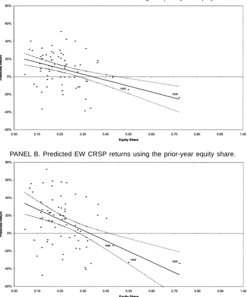
Our market return forecasts are presented in Table IX.20In a simple
uni-variate model, the equity share predicts negative returns for six years: 1929, 1930, 1934, 1982, 1983, and 1984. ~In three of these years, 1929, 1930, and 1984, real returns actually were negative.!The first two columns show data on the equity share in those six years. Columns~3!and~4!show the forecast return and its standard error. Columns~5! and ~6! test the hypothesis that predicted returns never fall below the sample average real government bond yield of 2.0 percent. This hypothesis is rejected at the five percent level for 1929, 1930, and 1984 equal-weighted and value-weighted returns and also for 1934 equal-weighted returns. Columns ~7! and ~8! test the hypothesis that predicted returns never fall below zero. This hypothesis is less theoret-ically motivated than the hypothesis of a non-negative risk premium, but it is also a lower hurdle for market efficiency to pass. Nevertheless, this hy-pothesis is still rejected at the five percent level for 1929 and 1930 value-weighted and equal-value-weighted returns and also for 1984 equal-value-weighted returns. These results can be compared to Kothari and Shanken’s~1997!finding that B0M forecasts significantly negative returns for only one year, 1930, and
then at the 10 percent level.
The results are presented graphically in Figure 4. They apply to columns ~7! and ~8! of Table IX. The solid line shows predicted value-weighted re-turns in Figure 4A for the observed range of the prior-year equity share. Figure 4B shows predicted equal-weighted returns. The dashed lines contain a 90 percent confidence interval for the predicted return. In the region where the top dashed line falls below zero, we can reject non-negative returns at the five percent level. Figure 4A shows this for 1929 and 1930, and Fig-ure 4B shows this for 1929, 1930, and 1984. We also plot the actual returns. Many of the actual returns fall outside of the 90 percent confidence interval. Because the equity share explains only about 12 percent in the variation in value-weighted returns, the confidence interval for individual returns is con-siderably larger than the confidence interval for the mean return.
19See Boudoukh, Richardson, and Smith~1993!for an alternative approach to testing the hypothesis of a nonnegative risk premium. They report evidence of a reliably negative risk premium during periods of high expected inf lation and downward-sloping term structures.
20In the tests in Table IX, we assume that the predicted return is normally distributed. The predicted return will be asymptotically normal regardless of the distribution of returns, but it will only be normal in a small sample if the returns themselves are normally distributed. For value-weighted returns, we cannot reject the hypothesis of normality using a skewness-kurtosis test. The equal-weighted returns, by contrast, have skewness and excess kurtosis. For this reason, the equal-weighted results must be viewed as an approximation.
T able IX T ests for Nonnegative Expected Returns T ests fo r nonnegative predicted returns using OLS reg ressions of annual real equity market returns ~ RE ! on the equity share in total new issues ~ S ! . The hypothesis test is ZREt 5 a 1 bS t 2 1 n H0 : ZR.E 0 Hats denote predicted values. Equity market returns are returns on the CRSP value-weighted ~ VW ! and equal-weighted ~ EW ! por tf olios. Returns are expressed in percentage terms. The equity share in new issues is standardized to have zero mean and unit var iance. The hypothesis p -values are shown using heteroskedastic ity robust standard errors. Actual returns are real returns created using the Consumer Pr ice Index from Ibbotson Assoc iates ~ 1998 ! . The sample average real government bond y ield ORf is 2.0 percent. Actual Return St2 1 Predicted Return ZRE . ORf ZRE . 0 Y ear REt ~% ! Equity Share ~ 1 ! Stdzd. Equity Share ~ X ! ~ 2 ! ZREt ~ % ! ~ 3 ! se ~ ZREt ! ~ % ! ~ 4 ! t -Statistic ~ 5 ! p -V alue ~6! t -Statistic ~ 7 ! p -V alue ~8! Panel A: VW CRSP 1930 2 23.77 0.72 4.64 2 25.50 8.85 2 3.1 1 0.001 2 2.88 0.002 1929 2 14.73 0.50 2.61 2 10.46 5.18 2 2.40 0.008 2 2.02 0.022 1984 2 0.65 0.43 2.00 2 5.91 4.16 2 1.90 0.029 2 1.42 0.078 1934 2.22 0.40 1.74 2 3.96 3.74 2 1.59 0.056 2 1.06 0.145 1983 18.21 0.36 1.41 2 1.51 3.26 2 1.08 0.141 2 0.46 0.321 1982 15.93 0.36 1.38 2 1.34 3.23 2 1.03 0.151 2 0.41 0.339 Panel B: EW CRSP 1930 2 33.63 0.72 4.64 2 46.69 15.67 2 3.1 1 0.001 2 2.98 0.001 1929 2 32.79 0.50 2.61 2 20.10 8.64 2 2.56 0.005 2 2.33 0.010 1984 2 13.91 0.43 2.00 2 12.06 6.64 2 2.12 0.017 2 1.82 0.035 1934 16.97 0.40 1.74 2 8.61 5.82 2 1.82 0.034 2 1.48 0.070 1983 32.65 0.36 1.41 2 4.28 4.87 2 1.29 0.098 2 0.88 0.189 1982 20.34 0.36 1.38 2 3.98 4.80 2 1.24 0.107 2 0.83 0.204