Spherical Correlation of Visual Representations for 3D Model Retrieval

Noname manuscript No. (will be inserted by the editor)

Spherical Correlation of Visual Representations for 3D Model

Retrieval

Ameesh Makadia · Kostas Daniilidis

the date of receipt and acceptance should be inserted later

Abstract In recent years we have seen a tremendous growth in the amount of freely available 3D content, in part due to breakthroughs for 3D model design and ac-quisition. For example, advances in range sensor tech-nology and design software have dramatically reduced the manual labor required to construct 3D models. As collections of 3D content continue to grow rapidly, the ability to perform fast and accurate retrieval from a database of models has become a necessity.

At the core of this retrieval task is the fundamen-tal challenge of defining and evaluating similarity be-tween 3D shapes. Some effective methods dealing with this challenge consider similarity measures based on the visual appearance of models. While collections of rendered images are discriminative for retrieval tasks, such representations come with a few inherent limita-tions such as restriclimita-tions in the image viewpoint sam-pling and high computational costs. In this paper we present a novel algorithm for model similarity that ad-dresses these issues. Our proposed method exploits tech-niques from spherical signal processing to efficiently evaluate a visual similarity measure between models. Extensive evaluations on multiple datasets are provided.

Keywords 3D shape retrieval·Visual similarity· Spherical Fourier transform

Ameesh Makadia

Google Research New York, New York, NY 10011 E-mail: [email protected]

Kostas Daniilidis

Department of Computer Science

University of Pennsylvania, Philadelphia, PA 19104 E-mail: [email protected]

1 Introduction

Laser-scanned objects, CAD models, and even image-based reconstructions are just a few of the sources con-tributing to rapidly growing, publicly available 3D model collections. Along with these vast 3D collections comes the need for a fast, large-scale model retrieval and match-ing system.

At the core of any content-based model retrieval engine lies the challenge of computing 3D shape simi-larity. Many of the difficulties in this task can be iden-tified as either global or local. Any shape representa-tion or similarity measure must compensate for global variations such as change in scale, orientation, etc. The second big challenge lies in local variations caused by object articulations or perturbations to local surface ge-ometry. Such variations can be attributed to noise or even modeling technology. For example, a polygonal mesh obtained from laser data will be quite different from a polygonal model of the same object designed by a human.

3D shape matching for retrieval has been a topic of ongoing research leading to many interesting tech-niques [1–11], all of which address the challenges men-tioned above to various degrees. In this work we are inspired by the family of methods which compare 3D models based on their visual similarity [1, 9]. For ex-ample, [1] has shown state-of-the-art retrieval and clas-sification results on standard benchmarks. The premise behind this approach is a 3D model representation con-sisting of a collection of images rendered from var-ious viewpoints. Although it may be a bit surprising that a collection of 2D images provides better discrim-ination than features based on 3D geometric informa-tion, a closer look will reveal two possible reasons for the strength of visual representations. First, rendering

views of a model circumvents the problem of dealing with complex, noisy, and possibly corrupt local 3D sur-face geometry. Second, if two categories of 3D models can be differentiated even by one particular discrimina-tive view, a sufficient sampling of renderings is likely to capture this distinguishing information.

However, despite their high performance relative to other retrieval methods, the image-based methods present their own challenges and limitations. For ex-ample, the Light Field Descriptor (LFD) of [1] is a rep-resentation that is not invariant to model orientation. Thus, there is a high computational cost that comes with evaluating a distance measure for many possible rotational alignments between models.

The inspiring idea of our work has first been drafted in [12], where a very preliminary formulation was de-veloped. In this paper we present methods for 3D shape comparison and retrieval that are built upon a visual representation of models. Specifically, similar to [1], our representation is a collection of silhouette images rendered from various viewpoints on the sphere sur-rounding the model. We define model similarity as the cross-correlation of these rendered silhouette image col-lections. Our primary contributions are in the formu-lation and efficient evaluation of this cross-correformu-lation similarity measure. We will show how model similar-ity can be evaluated efficiently using techniques from spherical harmonic analysis, taking advantage of the fact that spherical correlation is equivalent to multipli-cation in the spherical Fourier domain. Furthermore, our model comparison method can be extended in a simple and intuitive way to develop an iterative, coarse-to-fine model retrieval system for large collections of models. A thorough experimental evaluation of our pro-posed methods is presented for multiple challenging datasets, and the results show consistently state-of-the-art or near-state-of-the-state-of-the-art performance.

2 Prior work

Content-based 3D model retrieval continues to be an important practical as well as fundamental problem. From the practical perspective, many large web repos-itories (e.g. 3D Warehouse1_{) ignore shape content for} model search, which often leads to search results of limited success and applicability. Many researchers have proposed to address the problem of 3D similarity for the task of model retrieval, and what follows is a brief overview of just a few of the existing methods in the literature.

Global spherical representations are the most natu-ral (and common) representations for 3D models. The

1 _{http://sketchup.google.com/3dwarehouse/}

Extended Gaussian Image (EGI, [7]) was perhaps the earliest such representation, but there exist many others such as the Complex EGI [6], spherical distributions of shape area [5], radial distance functions [3, 4], and the Light Field Descriptor [1], just to name a few. Less common is the case where the underlying representa-tion is a 3D grid (see [2,13] for examples). A large sub-set of methods based on spherical representations uti-lize a Spherical Fourier representation to build model descriptors (see [2, 4] for examples).

On the opposite end of the spectrum exist those methods where 3D shapes are represented by local fea-tures. Spin images [14,15] and 3D Shape Contexts [16– 18] are examples where surface points are described by shape distributions of a local neighborhood. While lo-cal descriptors make it easier to deal with object articu-lations or missing parts, there is the added challenge of obtaining accurate correspondences. Recently [9] in-corporated local SIFT features [19] from rendered depth images into a traditional document retrieval bag-of-features approach to circumvent the direct correspondence prob-lem.

One of the challenges for shape matching is the wide variety of transformations that must be accounted for when comparing 3D models. In this regard, most of the approaches we have mentioned above can be di-vided into two categories. The first category contains those approaches where invariance to the possible trans-formations are built directly into the model represen-tation or the extracted descriptors. The second cate-gory contains those approaches that address the possi-ble transformations of a model at the time when model descriptors are being compared. For example, the most common transformations to which any 3D retrieval en-gine must be invariant are global changes in size (scale), position (3D translation), and orientation (3D rotation). Most of the approaches we have discussed above pro-pose methods to generate 3D model descriptors which have built-in invariances (i.e. any scaling, translation, or rotation of the 3D model will not alter the result-ing model feature descriptor). There are a number of ways this can be achieved. The most direct is to use descriptors that are inherently invariant to such trans-formations. For example, histograms of distances be-tween point pairs [8], or histograms of distances from surface points to the center of mass [5], are invariant to both rotation and translation. For those methods where the underlying representation is not invariant to certain transformations, simple measures can be taken: Scale can be normalized by isotropic scaling of a model to fix the average distance from surface points to the cen-ter of mass, for example. Translation can be normal-ized by shifting the model so that the center of mass

aligns with the origin. A simple way to factor out ori-entation is to use PCA-alignment, where the principal axes of a model are aligned with some common refer-ence frame. This type of PCA-alignment is commonly used for spherical or 3D grid representations where the model orientation is difficult to factor out. For spherical representations, an alternative to PCA-alignment is to extract general properties of a spherical function that are invariant to 3D rotations. For example, it is well-known that the magnitudes of Spherical Fourier coef-ficient vectors are invariant to rotation (see [2] for an application to 3D model comparison).

The benefit of encoding transformation invariance into 3D model descriptors is that such features can be directly compared using traditional distance measures. Nearest neighbor retrieval over thousands of models is still a fairly efficient computation when the pairwise distance measure is theL2distance between small fea-ture vectors, for example. Furthermore, it is straightfor-ward to utilize powerful classification machinery (e.g. an SVM classifier) with such features.

The problem with encoding invariance directly into the descriptors is that it often comes at a cost. As a general rule, the more invariance captured by a feature the less discriminative the descriptor. Another problem comes from possible inaccuracies in the methods. For example, orientation normalization using PCA-alignment has been shown to be inaccurate [20]. The alternative to building invariant descriptors is to address possible model transformations at the time of similarity (or dis-tance) computation. This allows one the freedom to build very robust and discriminative features from 3D models. However, the penalty is that there is a compu-tational disadvantage when descriptors are compared since the possible transformations must be accounted for. Typically this is addressed by an optimization or search over transformation parameters. For example, the Light Field Descriptor [1] represents a 3D model with a collection of rendered silhouette images. When two models are compared their respective silhouette collections must be compared for all possible 3D ro-tational alignments.

As our work in this paper builds on a visual model representation, it is closely related to the Light Field Descriptor of [1]. Thus, in the following section we will summarize the approach of [1] and highlight some of the existing limitations which are addressed in this paper.

3 Light Field Descriptors (LFD)

The method of [1] can be described as having three steps: First, given a 3D model, a collection of

silhou-ette images are rendered from multiple viewpoints sur-rounding the model. Second, features are extracted for each image. These features are used for pairwise com-parison of images. Third, for the comcom-parison of two 3D models, the pairwise distances between the models’ re-spective image collections are aggregated to provide a composite distance. This computation is then repeated for multiple rotations, and the minimum composite dis-tance is selected as the final disdis-tance between the mod-els. In the following subsections we will attempt to fill in many of the details of this approach.

3.1 Silhouette viewpoints

There are a few constraints which help determine the viewpoints from which silhouette images are rendered given a 3D model. Ideally, the viewpoints should be distributed “uniformly” over the sphere, to limit redun-dancy. Furthermore, the silhouettes from two different models will be compared pairwise for a set of 3D tations. This implies that there must exist some 3D ro-tations which map any viewpoint onto another (tran-sitivity), while also mapping the collection onto itself. For a collection ofN viewpoints (N > 2), the set of rotations that satisfy this constraint make up a finite subgroup of the 3D rotation groupSO(3). The finite subgroups of SO(3) are the cyclic groups, the dihe-dral groups, and the symmetry groups of the Platonic solids [21]. Although the cyclic and dihedral groups do not limit the number of silhouette vertices, the cor-responding rotations will cover only a small subspace ofSO(3). The Platonic solid with the most vertices is the regular dodecahedron (20 vertices). The dodecahe-dral group (often referred to by it’s dual, the icosahe-dral group), has order 60. In other words, for the con-figuration of 20 vertices aligned with the vertices of a dodecahedron, there are 60 unique 3D rotations which will map this set of 20 vertices onto itself. We should note that in practice only 10 silhouettes are used since vertices pand−pprovide identical information. The collection of 10 silhouettes, along with their individual silhouette descriptors, constitute the Light Field De-scriptor. A denser sampling of the viewpoint space is obtained by replicating the constellation of 10 silhou-ettes at small rotational offsets from the initial position.

3.2 Silhouette descriptors

A rendered silhouette image is a binary image with a single connected component. Lacking any appearance information, purely shape-based descriptors are used for the comparison of silhouettes.

The Zernike moment descriptor is obtained by pro-jecting the 2D silhouette onto a set of circular, com-plex Zernike polynomials of increasing degree. A few examples of Zernike polynomials are shown in figure 1. Degree = 0 Order = 0 Degree = 1 Order = 1 Degree = 2 Order = 0 Degree = 2 Order = 2 Degree = 3 Order = 1 Degree = 3 Order = 3 Degree = 4 Order = 0 Degree = 4 Order = 2 Degree = 4 Order = 4

Fig. 1 Nine Zernike polynomials (see [22] for details). The polynomials are shown for various degrees and orders. The poly-nomials are complex, so we are only showing the real component here. Colors closer to red are higher values (positive), while col-ors closer to blue are lower values (negative). The polynomials are defined on the circle, so the region outside the circle should not be considered. The(0,0)polynomial is uniform since a pro-jection onto this is equivalent to just an integration of the input function over the circle.

In total, the magnitude of 35 coefficients are kept for the descriptor.

The contour distance function r(θ) measures the distance from the silhouette centroid to the contour. An example of a silhouette image along with its extracted contour and corresponding distance function are shown in figure 2.

Since r(θ) is a periodic function on the circle, it is natural to examine its Fourier transformr(k)ˆ . The magnitude of 10 coefficients are retained for the de-scriptor.

Both the Zernike moment descriptor and the con-tour distance descriptor were evaluated extensively in [22], where it was shown an integrated approach utiliz-ing both descriptors performed well for image retrieval tasks. 50 100 150 200 250 50 100 150 200 250 0 50 100 150 200 250 300 350 400 30 40 50 60 70 80 90 θ

Distance from centroid

Contour Distance Function

Fig. 2 On the top left is a sample silhouette obtained from

ren-dering a 3D model of a human hand. On the top right we show the detected contour (obtained by a tracing algorithm) in green. The centroid of the shape is given by the green circle in the mid-dle of the hand. The green circle intersecting the shape contour specifies the first detected point along the contour, which also acts as the starting reference point for generating the contour distance function. The resulting contour distance function, mea-suring the distance of the contour points to the centroid, is shown in the bottom plot.

3.3 Model comparison

Given Light Field Descriptors for two models, there are 60 possible rotational alignments that must be consid-ered. The final 3D model distance is the minimum dis-tance over all Light Field Descriptor pairs for all pos-sible rotational alignments.

To speed up comparisons and retrieval from large databases, a multi-stage comparison approach is pro-posed in [1]. There are four controllable parameters: (versus accuracy):

1. Number of silhouettes. The number of images (up to ten) used in the comparison can be varied. 2. Number of LFDs can be varied.

3. Quantization of silhouette descriptors. Feature vec-tors can be quantized so that each coefficient is rep-resented with 4 or 8 bits, for example.

4. Subset of feature vectors. Distances can be com-puted using a subset of the feature vector coeffi-cients.

At each stage of the iterative model comparison, the above parameters are varied to provide additional ac-curacy, the basic idea being many models can be dis-carded after each iteration. For details of the proposed six-stage retrieval process see [1].

3.4 Limitations

The viewpoint configuration described above is tightly coupled with the set of possible rotational alignments. It is not simple to vary the number or position of view-points, or the number or samples of 3D rotations in-dependently. For example, increasing the number of rotational alignments evaluated while keeping the sil-houette viewpoints fixed implies silsil-houette (or feature) interpolation, however there is no clear approach for this.

The full comparison, even for just 100 silhouettes per model, is too computationally expensive for a database search. However, the proposed six-iteration method is fairly complex and seems a bit ad-hoc and arbitrary. There does not exist a clear intuition behind the deci-sions made during each stage. Combined with an ab-sence of a thorough evaluation, the motivations behind this process, along with the performance contributions from each parameter, are unclear.

Inspired by the discriminative strength of visual model representations, we present our model comparison tech-nique and address the key issues discussed above in the following sections.

4 Efficient 3D model comparison

In this section we will detail our proposed 3D model comparison technique. The outline is as follows: In section 4.1, we describe silhouette generation and fea-ture extraction. In section 4.2 we will define a similar-ity measure for comparing two models, and in 4.3 we show how this similarity measure can be evaluated effi-ciently borrowing techniques from spherical harmonic analysis. Section 4.4 covers the sampling requirements of our approach. In sections 4.5 and 4.6 we summarize the algorithm and provide some analysis and observa-tions.

4.1 Silhouette rendering and feature extraction

Our 3D model representation is a collection of silhou-ette images rendered from viewpoints surrounding the model. Consider a 3D model centered at the origin. For any sphere pointp∈S2_{, we can render a silhouette via} an orthographic projection of the model onto the plane tangent to the sphere atp. In this way we generate sil-houette images for any collection of spherical coordi-nates (we will discuss the number of silhouettes and their locations in subsequent sections). Furthermore, each silhouette we obtain will be represented by a fea-ture vector describing its shape. Although we have a

flexibility in selecting this feature vector, for compar-ison we will use the45-dimensional Zernike and con-tour descriptor as in [1].

4.2 Similarity measure

For the moment, let us consider that our collection of silhouettes is not finite, but rather we have obtained im-ages and feature vectors from all points on the sphere. In this continuous setting, we have a N-dimensional feature vector at each point on the sphere (as described above, in our experimentsN = 45). Formally, we will write this silhouette feature representation as M(p)i,

wherepis a sphere point (p∈ S2_{) andiis the index} into the N-dimensional feature vector that describes the silhouette obtained from viewpointp. To compare two 3D models, we define their similarity as the cross-correlation of their feature representations:

Gc= N X i=1 Z p∈S2 M1(p)iM2(p)idp (1)

In practice we evaluate a normalized cross-correlation, but for simplicity we leave out the normalization terms in our description here. Note, equation 1 evaluates a similarity measure over the two model representations M1 andM2 in their native orientations. However, as we do not know the correct rotational alignment, we must consider all possibilities:

Gc(R) = N X i=1 »Z p∈S2 M1(p)iM2(RTp)idp – , R∈SO(3) (2) HereGc(R)measures the cross-correlation for all

pos-sible 3D rotational alignmentsR∈SO(3). We define the similarity between two models as the maximum value of Gc(R). Computationally, evaluating Gc(R)

directly is cumbersome. For each 3D rotation we must rotate one model representation (M2) and perform a 3D integration. In the next subsections we see how to evaluateGc(R)efficiently.

4.3 Similarity evaluation

To efficiently evaluate the model similarity function Gc(R)from equation 2, we recognize that the inner

in-tegral fits the definition of a correlation between func-tions defined on the sphere. Isolating the inner integral gives

G(R) = Z

p∈S2

M1(p)M2(RTp)dp, R∈SO(3) (3) To evaluate G(R), we adopt an approach similar to those described in [23–28], which show that the spheri-cal correlation integral is equivalent to a multiplication

of Fourier transforms. We provide a brief summary of this result here, but readers are referred to [24, 25] for reference.

In traditional Fourier analysis, periodic functions on the line (or equivalently functions on the circleS1_), are expanded in a basis spanned by the Eigenfunctions of the Laplacian. Similarly, the Eigenfunctions of the spherical Laplacian provide a basis forM(p)∈ L2_(S2₎ (here L2 _{denotes square-integrability). These} Eigen-functions are the well known spherical harmonics (Yl

m:

S2_{7→C), which form an Eigenspace of harmonic} ho-mogeneous polynomials of dimension2l+ 1. Thus, the 2l+ 1spherical harmonics for eachl≥0form an or-thonormal basis for anyM(p)∈ L2_(S2_{). The} spheri-cal harmonic for degreeland orderm(l ≥ 0,|m| ≤

l, l, m∈Z), is given as Yl m(θ, φ) = (−1) m s (2l+ 1)(l−m)! 4π(l+m)! P l m(cosθ)e imφ

Note we are usingpand(θ, φ)interchangeably to de-note points on the sphere. In the above equationPl

mare

the associated Legendre functions and the normaliza-tion factor is chosen to satisfy the orthogonality con-straint. Readers are referred to [29, 30] for a in-depth treatment of spherical harmonics. Any functionM(p)∈ L2_(S2_{)can be expanded in a basis of spherical} har-monics: M(p) =X l∈N l X m=−l ˆ Ml mYml(p) (4) ˆ Ml m= Z p∈S2 M(p)Yl m(p)dp (5) TheMˆl

mare the coefficients of the Spherical Fourier

Transform (SFT). Henceforth, we will useMˆl _to

an-notate vectors in C2l+1 _{containing all coefficients of} degreel, ordered from−lthrough+l.

As functions on the sphere can be expanded in spher-ical harmonics, functions defined on the rotation group can be expanded in the irreducible unitary representa-tions of the rotation group. ForG(R) ∈ L2_(SO(3)), we can write its Fourier expansion as

G(R) =X l∈N l X m=−l l X k=−l ˆ Gl mkU l mk(R) (6) ˆ Gl mk= Z R∈SO(3) G(R)Ul mk(R)dR (7) TheGˆl

mk, withm, k=−l, . . . , lare the(2l+1)×(2l+

1)coefficients of degreelof theSO(3)Fourier trans-form. TheUl

mk(R)are the elements of the irreducible

matrix representations ofSO(3). We will writeUl_(R)

for the(2l+1)×(2l+1)matrix representation at degree

l, andGˆl_{for the matrix ofSO(3)Fourier coefficients}

at degreel.

There is a close relationship between the Fourier representation of functions on the sphere and the ma-trix representations Ul_{(R). Specifically, as spherical}

functions are rotated by elements ofSO(3), their Fourier coefficients are “modulated” by the irreducible repre-sentations ofSO(3):

M(p)7→M(RT_p)⇐⇒Mˆl_7→Ul_(R)T_Mˆl ₍₈₎

This relationship, along with the orthogonality of the spherical harmonics, allows us to expand equation 3 in terms of the corresponding Fourier transforms:

ˆ Gl= ˆM1 l ( ˆM2 l )T ₍₉₎

This shows that theSO(3)Fourier coefficients ofG(R) can be obtained as a matrix product between the coef-ficient vectors of the two spherical functionsM1and M2.

4.4 Viewpoint sampling

A fast discrete algorithm for the spherical Fourier trans-form, based on a separation of variables technique, can be attributed to [30]. The complexity of the transform is O(L2_log2_{L), where L is the “bandwidth” of the} spherical function. In practice, the selection ofL sim-ply specifies that only those coefficients of degree less

thanLwill be retained from the Fourier transform. The sampling requirement to achieve the noted complexity is that2Lsamples must be placed uniformly in each spherical coordinate (i.e.2Lsamples in colatitude, and 2Lsamples in azimuth). Figure 3 shows the effect of this sampling constraint on the distribution of spherical silhouette viewpoints.

A B C

Fig. 3 On the left (A) is a representation of a uniformly sampled

spherical grid, with 16 samples spaced uniformly in each dimen-sion. This is the sampling requirement for a fast spherical Fourier transform at bandwidthL = 8. (B) depicts the corresponding sample support regions as they appear on the sphere. The high-lighted bins correspond to the highhigh-lighted row in (A). The circles in (C) specify the actual sample locations on the sphere.

Similar to the spherical transform, there exists a separation of variables technique for a fast discreteSO(3) Fourier transform [24]. The complexity for such a tech-nique isO(L3_log2

L), where as beforeLis the func-tion bandwidth. This fast discrete transform is given for a standard Euler angle parameterization ofSO(3). In particular, the three anglesα, γ ∈ [0,2π)andβ ∈

[0, π], can generate any 3D rotation throughR=Rz(γ)Ry(β)Rz(α).

HereRzandRyrepresent rotations about theZandY

axis, respectively.

For a fast discrete SO(3) transform of a function with bandwidthL, the sampling theorem requires2L samples uniformly spaced in each of the three Euler angles α, β, and γ. As with the spherical transform, this uniform sampling in Euler angles leads to a non-uniform sampling in rotation space.

The fast spherical and rotational Fourier transforms detailed in [24, 30] provide us the machinery necessary for evaluating the spherical correlation integral (equa-tion 3) in the Fourier domain (equa(equa-tion 9).

4.5 Pairwise model comparison summary

We now summarize our pairwise 3D shape comparison formulation as detailed above, and provide some prac-tical considerations and complexity analysis. The only parameter we need to set is the frequency bandwidth L, which will initially dictate the sampling frequency in the silhouette viewpoint space, as well as the 3D ro-tation space.

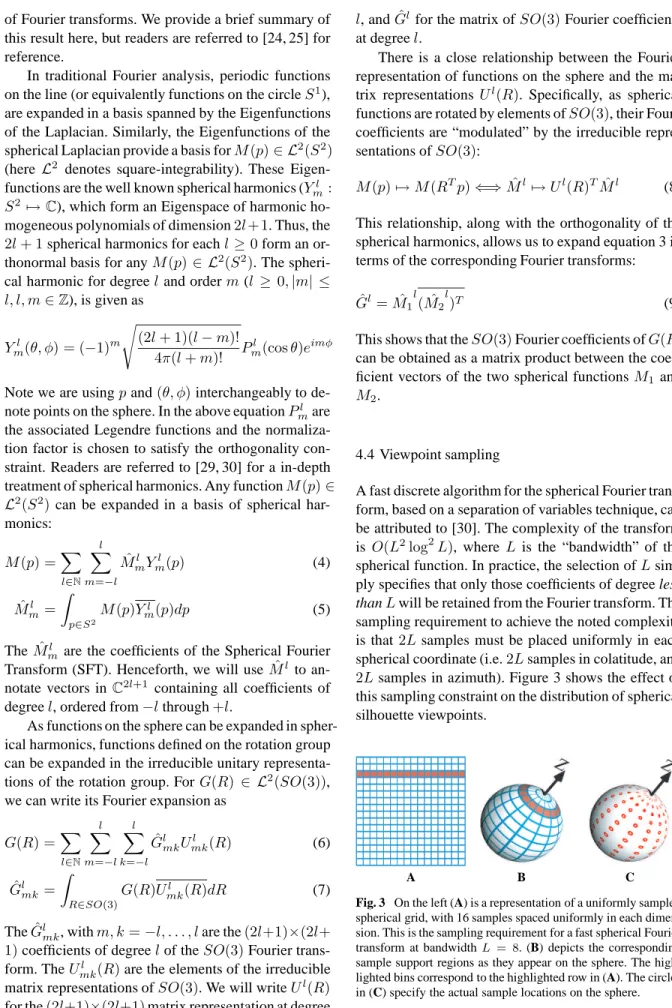
Given two models which we wish to compare, the first step is generating silhouette images and features from each model. As per the Fourier sampling theo-rem, given a bandwidthL, we will need to generate 2L×2L = 4L2_{orthographically rendered silhouette} images from each model. For any silhouette viewpoint p ∈ S2_{, the antipodal point−p provides redundant} information. Thus in practice, we only need to ren-der half the silhouettes (a total of2L2 _images). Fig-ure 4 provides an example of a 3D model and its sil-houette images. Subsequently, each silsil-houette image is replaced with itsN-dimensional feature vector repre-sentation. After feature extraction, we have our initial model representationsM1(p)iandM2(p)i.

To obtain the Fourier domain representation ofM(p)i,

we must take a separate spherical Fourier transform for each silhouette feature indexi= 1, . . . , N, leaving us with the coefficients ( ˆMl

m)i. For a fixed L, we will

have a total ofN L2 _{Fourier coefficients. As we} ob-served earlier, the spherical model representation ex-hibits the even propertyM(p)i = M(−p)i. This

re-dundancy translates to the Fourier space: ( ˆMl

m)i =

0,∀lodd. Additionally, the spherical Fourier transform

φ= 0◦ _{φ= 60}◦_{φ= 120}◦_{φ= 180}◦_{φ= 240}◦_{φ= 300}◦

θ= 15◦

θ= 45◦

θ= 75◦

Fig. 4 An example of a 3D model and its corresponding

silhou-ette images. On the top is a 3D model downloaded from Google’s 3D Warehouse. For a bandwidthL= 3,2L2 _{= 18silhouettes}

will be rendered. In this figure, the top row corresponds to sil-houettes from viewpoints with fixed colatitude (15◦_{) but varying}

azimuth.

is defined generally for complex-valued functions. For real-valued functions the coefficient vectors( ˆMl

m)i

ex-hibit an hermitian property:( ˆMl

−m)i= (−1)m( ˆMml)i.

These two facts show that only the coefficients( ˆMl

m)i

forl even andm ≥ 0are necessary, greatly reducing the storage space of our Fourier representation.

The Fourier representations of the two models,( ˆM1

l

m)i

and( ˆM2

l

m)i, are the necessary input for evaluating the

correlation similarity measure. From equation 9, we showed that theSO(3)Fourier coefficients ofGc(R)

can be obtained in the spectral domain as:

ˆ Gc l = N X i=1 ˆ M1 l i( ˆM2 l i)T (10)

To obtain the samples of our desired correlation func-tion Gc(R), we must take an inverse SO(3) Fourier

transform as a final step. Note, we have the option of taking the inverseSO(3)transforms before or after the summationP

i. In other words, if we let ISOFT(.)

the following are equivalent: Gc(R) = N X i=1 ISOFT ˆ M1 l i( ˆM2 l i)T (11) =ISOFT N X i=1 ˆ M1 l i( ˆM2 l i)T ! (12)

While these computations have numerically identical results, there is a clear advantage to equation 12. Evalu-ating equation 11 hasO(N L3_log2_{L)complexity. This} comes from havingN separateSO(3) Fourier trans-forms, each of which has complexityO(L3_log2_{L). On} the other hand, evaluating equation 12 requires only one Fourier transform. Although the inner summation PN

i=1over coefficient vectors has complexityO(N L3), the constant factor is minimal. The total complexity of equation 12 isO(N L3_)+O(L3_log2_{L) =O(L}3_(log2_L+ N)). In practice, the computational burden lies in the Fourier transform, and thus we see a speedup by a fac-tor of approximately 10 when evaluating equation 12 in place of equation 11. We can also compare this com-plexity against the original definition ofGc(R)as given

in equation 2. To evaluate equation 2 in the spatial do-main would have a complexity ofO(N L5_{)(this would} also be the complexity of evaluating [1] for similar numbers of silhouette and rotation samples).

In the final step, the maximum value from the sam-ples ofGc(R)(as obtained via equation 12) is selected

as the similarity score between the two input models.

4.6 Sampling flexibility

We will now discuss how our approach addresses one of the key issues brought up earlier, namely the de-pendence between the number of silhouette viewpoint samples and the number of samples in the 3D rotation space. First, we note that our development allows for an arbitrarily dense sampling of the viewing sphere and 3D rotation space. For a fixed bandwidth L we will have 2Lsilhouette viewpoint samples uniformly spaced in the each of the two spherical coordinates, as well as 2L samples uniformly spaced in each of the three Euler angles. This straightforward formula-tion allows us to achieve a sampling where the maxi-mum distance between any silhouette viewpoint and its nearest neighbor is arbitrarily small (similarly with 3D rotations), simply by varying the bandwidthL.

Furthermore, we can achieve an independence be-tween the number of silhouette samples and the num-ber of 3D rotations samples ofGc(R). In other words,

we are not forced to have the same bandwidth parame-terLfor both the silhouette model representationM(p)i

and the 3D correlation functionGc(R). For example,

assumeL′_{is the chosen bandwidth of the model} repre-sentationsM1,2(p)i, which implies a total of2L′2

sil-houette images. LetL′′ _{> L}′_{. We can easily generate} ˆ

Gc l

forl= 0, . . . , L′′_{−1as in equation 10 by setting} ˆ

Gc l

= 0,∀L′ _{≥ l < L}′′_{. In this approach, the extra} samples obtained in the 3D rotation space by having a higher bandwidthL′′_{are interpolated using the Fourier} coefficients ofM(p)i up to bandwidthL′. Thus, our

approach provides a simple mechanism for indepen-dently varying the number of silhouette viewpoint sam-ples and the number of 3D rotation samsam-ples. If desired, many more samples ofGc(R)can be interpolated from

few silhouette images. Contrast this to a direct spatial approach (e.g. [1]), where there are strict dependen-cies between silhouette view samples and possible 3D rotations, and no simple mechanism for interpolation exists.

5 A natural coarse-to-fine estimation of similarity The development in the previous section presents a novel approach for determining the similarity between a pair of 3D models. Such a technique can be very important for an application such as 3D model retrieval, where the challenge is to identify the most similar models to a query from a very large database. In such a set-ting, it can be computationally infeasible to perform a full similarity evaluation between the query and every database model just to identify the few most similar models. Instead, when searching for nearest neighbors we would like to discard large numbers of candidate models with few computations. To this end, our model comparison approach can easily be extended to form an iterative coarse-to-fine evaluation of model similar-ity. The basic idea is very intuitive, and comes from the observation that the degree of a Fourier coefficient indicates the frequency component that is represented. In other words, a coarse estimation of similarity using only low-frequency signal information can be obtained by using only the low-degree Fourier coefficients. Sub-sequently, a higher precision can be achieved by intro-ducing high-frequency signal information in the way of the high-degree Fourier coefficients. To build a 3D model retrieval system for a large database of models, we can proceed as follows:

In a pre-processing step, each model in the database is represented with the Fourier coefficients( ˆMl

m)i at

some bandwidthL. Given a query model, the first iter-ation for retrieval involves evaluating a coarse similar-ity between the query and every database model. This coarse similarity is obtained by computingGc(R)at

some small bandwidthL′_{< L. Those models furthest} from the query can be discarded. In each subsequent

iteration, a finer similarity score is computed between the query and remaining database candidates by evalu-atingGc(R)at an increased bandwidth. In the final

it-eration a ranked list of nearest neighbors is created by evaluatingGc(R)at the full bandwidthLfor the few

remaining candidates. In this way we can discard the large majority of database models with limited compu-tation.

6 Rotational invariants

The model comparison and retrieval approaches we have presented above utilize representations that are not in-variant to 3D rotations. As we discussed earlier, a gen-eral alternative is to build rotational invariance directly into the model feature representation. Feature descrip-tors which are invariant to model transformations al-ways lead to faster comparison (since no search over the transformation space needs to be done online), and are also suitable for use with standard off-the-shelf clas-sification techniques (e.g. SVM classifiers). For sphere-based 3D model representations there are two ways to normalize for orientation. The simplest and most com-mon approach is to align the model’s principal axes with a fixed reference frame. An alternative to this PCA-alignment is to identify the rotation-invariant terms in the spherical Fourier domain (see [2,31] for details and other applications for such invariants). We saw earlier (equation 8) how the Fourier coefficients of a function transform under a 3D rotation of the original function. The Fourier analogue to 3D rotations are given by the matrix transformationsUl_{(R). We know that these}

uni-tary transformations will not alter the distribution of spectral energy among coefficient degrees:

||Ul_{(R) ˆM}l_||

2=||Mˆl||2,∀R∈SO(3)

where ||.||2 indicates L2 vector norm. We can build a rotation-invariant model feature vector by retaining only the magnitudes of the Fourier coefficient vectors (||Mˆl

i||). The total size of such a model descriptor is

⌊L

2⌋N. For example, consider a model for which we render a very large number of silhouettes (e.g.L= 17 means we must render 2L2 _{= 578 images).} Assum-ingN = 45 as we have used throughout this paper, our model representation is just one feature vector of 45∗8 = 360dimensions. The distance between two models is defined as the Euclidean (L2) distance be-tween their respective feature vectors.

7 Experiments

In this section we will study the effectiveness our pro-posed 3D model comparison technique with three

chal-lenging evaluations (the Princeton Shape Benchmark, the Shape Retrieval Contest in 2006, and a collection of models downloaded from Google’s 3D Warehouse). We begin with a study on the de-facto evaluation bench-mark for 3D shape retrieval, the Princeton Shape Bench-mark [32].

7.1 Princeton Shape Benchmark

The Princeton Shape Benchmark [32] provides a col-lection of 3D models designed for the standardized eval-uation of retrieval, matching, clustering, and recogni-tion algorithms. The database consists of 1814 man-ually categorized 3D models collected from the Web. The database is segregated into a training set consist-ing of 907 models and spannconsist-ing 90 model classes, and a test set consisting of the remaining 907 models and spanning 92 model classes. In the test set, the largest category contains 26 models (“potted plant”), and the smallest category contains 4 models (there are 17 cat-egories with just 4 models). Figure 5 shows a few ex-amples of models in the benchmark.

Fig. 5 Thumbnail images of six different models in the

Prince-ton Shape Benchmark [32]. The top row consists of thumbnails from the “potted plant” class, which constitutes the largest class in the PSB test set. The bottom row consists of thumbnails from the “Newtonian toy” class, which is one of 17 classes in the test set tied for having the fewest models (four).

To stay consistent with published evaluations on the benchmark, we restricted ourselves to evaluations over the 907 model test set. In principle, our approach is training-free, and thus could be evaluated over the entire 1814 model benchmark.

To evaluate the robustness of our method, we ini-tialize every 3D model with a randomly generated 3D

rotation before rendering model silhouettes. This is im-portant because although model orientation is unknown, it is quite common in the benchmark to see many mod-els that are aligned with the ground plane in their na-tive orientations. In order to provide a proper evalua-tion of our correlaevalua-tion-based method, a random rota-tion of each model will cancel out any orientarota-tion bias in the benchmark.

In general, evaluation over the test set is performed by removing one model to act as the query, and rank-ing the remainrank-ing models from most similar to least similar. This ranked list can be evaluated in a number of ways (a few of which we will detail below). Per-formance for a particular method or set of parameters is given by averaging the performance over all query models. The evaluation measures for the benchmark are as follows (see [32] for details):

1. Nearest Neighbor measures the accuracy of the first retrieved neighbor.

2. First Tier and Second Tier. The ratio of models in the query class that appear in the firstKresults. If |C| is the number of models in the query’s class, K =|C| −1for first tier andK = 2∗(|C| −1) for second tier.

3. E-measure is a combined measure of the precision and recall for a fixed number of results (here the evaluation neighborhood size is 32). The E-measure is defined as2/(_P1 + _R1), where precision (P) and recall (R) are defined in the usual document re-trieval way.

4. Discounted Cumulative Gain (DCG) is an evalua-tion measure of the entire ranked list that weights positive results at the top of the list higher than pos-itive results lower on the list.

The evaluation measures described above emphasize positive results earlier in the ranked retrieval. This is in line with the idea that for many search applications, users will often only be interested in the quality of the first few returned results. Perturbations towards the end of the list will have little effect on the perceived quality of the retrieval.

The performance criteria listed above were used to evaluate a number of existing 3D shape compari-son and retrieval algorithms in [32]. We have reprinted these published results along with the performance of our proposed model similarity measure in table 1.

We ran the retrieval algorithm for 8 different band-width parameters, ranging fromL = 3up toL= 17. In this setting, the selection of bandwidth was kept fixed for the entire algorithm (i.e. the same bandwidth Lwas used for feature generation and evaluating the correlation functionGc(R)). Our evaluation indicates

that we do see an improvement over the closest method,

0 0.2 0.4 0.6 0.8 1 0 0.1 0.2 0.3 0.4 0.5 0.6 0.7 0.8 0.9 1 Recall Precision Precision−Recall L = 17 L = 15 L = 13 L = 11 L = 9 L = 7 L = 5 L = 3

Fig. 6 Precision-Recall curves for our proposed shape

compar-ison algorithm on the Princeton Shape Benchmark test set. The evaluation code used to generate these plots was taken from the evaluation utilities provided with the benchmark [32]. As we can see, there is little variation in results between the lowest and highest bandwidths.

LFD [1]. Furthermore, we see close-to state of the art results at even lower bandwidth settings. Interestingly, the relative performance difference between retrievals run at the higher bandwidths (L≥9, for example) are very small. This fact can be clearly observed in figure 6, where we show precision-recall curves for the vari-ous bandwidth settings.

The gap in performance at various bandwidth set-tings indicates that our proposed coarse-to-fine scheme may prove just as effective as performing retrieval at the highest resolution ofL= 17. What remains to be determined are the specifics of the incremental coarse-to-fine retrieval. Based on the results in table 1 and fig-ure 6, we can do most of the ranking and similarity computation at the low bandwidths and use the high resolution bandwidth for a final “fine-tuning” (i.e. re-ranking) of a few models. What we would expect to see is that the DCG scores may not reach those of the highest bandwidth since DCG is a measure of the en-tire ranked listing. However, we would expect to see nearest-neighbor scores mostly unaffected.

We experimented with the following incremental scheme: first, the similarity scores are computed for all model pairs at the lowest bandwidth (L = 3). In the second pass, we identify the most similar20%, and re-rank these models by computing similarity atL= 5. In the third and final pass, we re-rank the1%most sim-ilar models at L = 17. The results are shown in ta-ble 2. As expected, the global measurements like DCG fell somewhere between the low and high-bandwidth results. Surprisingly, however, the nearest-neighbor re-sults outperformed all algorithms including the fullL=

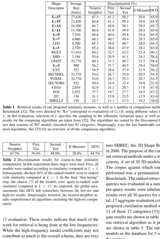
Shape Descriptor Storage Size (bytes) Discrimination (%) Nearest Neighbor First Tier Second Tier E-MeasureDCG L=17 27,630 67.3 41.2 50.2 29.6 65.9 L=15 21,420 66.8 41.1 50.2 29.6 65.9 L=13 16,200 66.7 40.8 50.1 29.5 65.7 L=11 11,700 66.8 41.0 49.9 29.4 65.6 L=9 7,920 66.8 40.6 49.8 29.4 65.5 L=7 4,860 66.3 40.1 49.4 29.3 65.0 LFD 4,700 65.7 38.0 48.7 28.0 64.3 L=5 2,520 65.4 38.6 47.9 28.1 63.8 REXT 17,416 60.2 32.7 43.2 25.4 60.1 SHD 2,184 55.6 30.9 41.1 24.1 58.4 GEDT 32,776 60.3 31.3 40.7 23.7 58.4 L=3 900 56.2 31.7 40.5 24.4 58.0 EXT 552 54.9 28.6 37.9 21.9 56.2 SECSHEL 32,776 54.6 26.7 35.0 20.9 54.5 VOXEL 32,776 54.0 26.7 35.3 20.7 54.3 SECTORS 552 50.4 24.9 33.4 19.8 52.9 CEGI 2,056 42.0 21.1 28.7 17.0 47.9 EGI 1,032 37.7 19.7 27.7 16.5 47.2 D2 136 31.1 15.8 23.5 13.9 43.4 SHELLS 136 22.7 11.1 17.3 10.2 38.6

Table 1 Retrieval results of our proposed similarity measure, as well as a number of comparison methods, on the Princeton Shape

Benchmark [32]. The rows denoted by “L=” correspond to evaluations ofGc(R)using different values for the bandwidth parameter

L. In this evaluation, selection ofLspecifies the sampling in the silhouette viewpoint space as well as the 3D rotation space. The results for the competing algorithms are taken from [32]. The algorithms are sorted by the Discounted Cumulative Gain Score. The test data consists of 907 models classified into 92 categories. Surprisingly, even the low bandwidth correlations are outperforming most algorithms. See [32] for an overview of all the comparison algorithms.

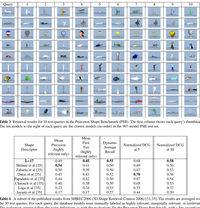
Nearest Neighbor First Tier Second Tier E-Measure DCG 67.5% 39.4% 48.0% 28.0% 64.7%

Table 2 Discrimination results for coarse-to-fine similarity

computation. In this experiment three stages were used. First, all models were ranked according to similarity computed atL= 3. Subsequently, the best20%of the ranked models were re-ranked with similarity computed atL = 5. In the final “fine-tuning” step, the closest1%of the models were again re-ranked with similarity computed atL = 17. As expected, the global mea-surements like DCG fell somewhere between the low-res and high-res results. Surprisingly, however, the nearest-neighbor re-sults outperformed all algorithms including the high-res compu-tation.

17evaluation. These results indicate that much of the work for retrieval is being done at the low frequencies. While the high-frequency model coefficients may not contribute as much to the overall scheme, they are very valuable as a “fine-tuning” mechanism for re-ranking the top results.

In addition to these quantitative results, we show some examples of the top retrieval results for various query models in table 3.

7.2 SHREC 2006

In addition to the extensive evaluation on the PSB, our correlation based shape retrieval algorithm was entered

into SHREC, the 3D Shape Retrieval Contest [33, 34] in 2006. The purpose of the contest was to study differ-ent retrieval methods under a wide variety of evaluation criteria. A set of 30 3D models served as the query set. The corpus against which ranked retrieval was to be performed was a permutation of the Princeton Shape Benchmark. The ranked retrieval lists for each of the 30 queries was evaluated in a number of ways. Individual per-query results were tabulated, as well as aggregate results over all 30 queries for each contest entry. In to-tal, 17 aggregate evaluation criteria were used, and our proposed correlation method was the top performer in 11 of these 17 categories [33]. A subset of the aggre-gate results are shown in table 4. Qualitative results of our retrieval algorithm as it performed in this contest are shown in table 5. The table shows the 10 closest models in the database for 5 of the 30 queries used in the contest.

An alternative to the correlation-based comparison approach is to encode rotation-invariance directly into the feature descriptor. This can be done by comput-ing rotation-invariant model descriptors as described in section 6. While the online comparison cost is much less (Euclidean distance of a small feature vector ver-sus spherical correlation), the discrimination performance is expected to be much worse. This is in fact the ob-served effect in figure 7. Given a ranked list generated from rotation-invariant feature vectors, we observe how

Query 1 2 3 4 5 6 7 8 9 10

Table 3 Retrieval results for 10 test queries in the Princeton Shape Benchmark (PSB). The first column shows each query’s thumbnail.

The ten models to the right of each query are the closest models (in order) in the 907-model PSB test set.

Shape Descriptor Mean Precision (highly relevant only) Mean First Tier (highly relevant only) Dynamic Average Recall Normalized DCG at 5 Normalized DCG at 50 L=17 0.49 0.45 0.55 0.68 0.58 Shilane et al [35] 0.54 0.41 0.50 0.69 0.56 Zaharia et al [35] 0.50 0.39 0.50 0.67 0.53 Daras et al [35] 0.45 0.43 0.52 0.70 0.56 Papadakis et al [35] 0.44 0.42 0.50 0.67 0.54 Chaouch et al [35] 0.40 0.38 0.50 0.68 0.53 Laga et al [35] 0.23 0.24 0.33 0.53 0.37 Jayanti et al [35] 0.17 0.17 0.27 0.44 0.30

Table 4 A subset of the published results from SHREC2006 (3D Shape Retrieval Contest 2006) [33,35]. The results are averaged over

the 30 test queries. For each query, the database models were manually labeled as highly relevant, marginally relevant, or irrelevant. The evaluation criteria follow the same definitions as with the evaluations for the Princeton Shape Benchmark, with a few exceptions. For a given query, if the recall ratio within the topineighbors is given asri, then the Dynamic Average Recall is defined as the mean over allri. Normalized DCG represents the Discounted Cumulative Gain divided by the ideal or optimal possible Discounted Cumulative Gain score. For more contest results see [33, 35], and for a detailed explanation of the evaluation criteria see [34]. Each entrant into the competition was allowed multiple entries, either to be used for different algorithms, or just different parameter settings for the same general approach. To be fair to the comparison methods, we have only shown here the best performing method in each evaluation column for all the entrants. For our proposed method, we are showing the results atL= 17.

many of the top-ranked models must be observed be-fore seeing50%of the topK models retrieved using our correlation similarity measure (the plot shows the median over all 30 queries). For example, in order to see 50 of the top 100 retrieved models using a corlation similarity, we have to examine the first 213 re-trieved models using rotation-invariant descriptors. As expected, the computational benefit of building invari-ance directly into the descriptor is offset by the loss in discrimination power.

7.3 Google 3D Warehouse

While the Princeton Shape Benchmark has become one of the standard evaluation datasets for 3D model re-trieval algorithms, the benchmark can be criticized for it’s lack of variation within classes in addition to other factors such as a lack of articulated object classes. We therefore evaluated our proposed model comparison method on a more challenging real-word dataset. This set con-sists of 772 3D models downloaded from Google’s 3D

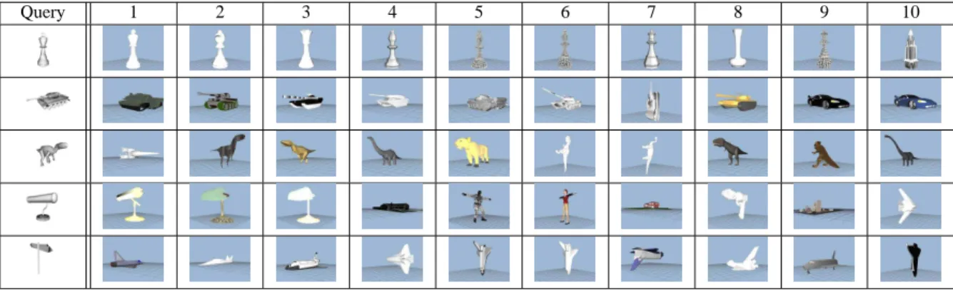
Query 1 2 3 4 5 6 7 8 9 10

Table 5 Top 10 retrieval results for 5 of the 30 queries from the SHREC 2006 contest. On the left column we show the query models,

and to the right of each query model are the 10 nearest neighbors in the database.

10 20 30 40 50 60 70 80 90 100 20 40 60 80 100 120 140 160 180 200 220

best K models in correlation method

Fig. 7 This plot shows how many models in the ranked list

(ob-tained by comparing rotation-invariant vectors) you need to tra-verse before finding50%of the bestKmatches in the ranked list obtained with the proposed correlation scheme. The plot shows the median over all test queries. For example,50%of the best 100 matches from the correlation method will appear in the first213matches from the ranked list obtained by comparing rotation-invariant model descriptors.

Warehouse, which is a repository for 3D models on the Web. All the models are grouped into a total of 25 classes. The categorization of models corresponds sim-ply to the search term used to find and the model. The largest category is “airplane” with 58 models, and the smallest is “fish” with only 6 models.

Figure 8 shows a few examples from the dataset. One of the biggest challenges posed by this repository is that individual model files can consist of multiple ob-jects. For example, the figure shows that the “garage” model consists of multiple structures in addition to the garage object (such as the ground plane).

Our primary evaluation criteria for this set was pre-cision versus recall. We averaged results over individ-ual classes, as well as over all 772 models. For compar-ison, we evaluated the method proposed by [13], where

Fig. 8 Samples of the 3D model dataset created from 3D

Ware-house. Each column shows samples from a single category. The three categories shown here are “stadium”, “plane”, and “garage”. These sample images indicate a few reasons why this collection is very challenging. For example, we see that there is a large variation in scale and complexity within and between cat-egories. Also, models on 3D Warehouse are not just individual objects as in the Princeton Shape Benchmark. Here individual model files such as the garage can consist of multiple pieces like the garage, ground plane, etc. This makes matching based solely on shape content very challenging.

3D Zernike descriptors are used to represent the mod-els. Note, for this dataset all of our similarity measure evaluations are performed atL= 11. Results averaged per class are shown in figure 9, while results averaged over all the models are shown in figure 10. The re-sults indicate consistently high performance for most classes of models in the set.

7.4 Timings

The algorithms proposed in this paper can play a big role in a system for 3D model search and retrieval. Hence, it is important to be aware of the execution times. There are two stages of computation. The pre-processing stage involves computing the model fea-tures. This is an offline step regarding database

cre-0 0.2 0.4 0.6 0.8 1 0.2 0.4 0.6 0.8 Recall Precision airplane (58) 0 0.2 0.4 0.6 0.8 1 0.2 0.4 0.6 0.8 Recall Precision bench (48) 0.2 0.4 0.6 0.8 1 0.1 0.2 0.3 0.4 0.5 0.6 Recall Precision bike (23) 0.2 0.4 0.6 0.8 1 0.1 0.2 0.3 0.4 0.5 Recall Precision bridge (35) 0.2 0.4 0.6 0.8 1 −0.1 0 0.1 0.2 0.3 0.4 Recall Precision castle (44) 0 0.2 0.4 0.6 0.8 1 0.1 0.2 0.3 0.4 0.5 0.6 Recall Precision chair (30) 0.2 0.4 0.6 0.8 1 −0.1 0 0.1 0.2 0.3 0.4 Recall Precision church (32) 0 0.2 0.4 0.6 0.8 1 0.1 0.2 0.3 0.4 0.5 0.6 Recall Precision computer (16) 0.2 0.4 0.6 0.8 1 0 0.1 0.2 0.3 0.4 Recall Precision door (11) 0 0.2 0.4 0.6 0.8 1 −0.1 0 0.1 0.2 0.3 0.4 Recall Precision fish (6) 0.2 0.4 0.6 0.8 1 0 0.1 0.2 0.3 0.4 Recall Precision garage (12) −0.2 0 0.20.4 0.6 0.8 1 1.2 0.2 0.4 0.6 0.8 1 Recall Precision guitar (37) 0 0.2 0.4 0.6 0.8 1 0.1 0.2 0.3 0.4 0.5 0.6 0.7 Recall Precision gun (48) 0.2 0.4 0.6 0.8 1 0 0.1 0.2 0.3 0.4 Recall Precision lamp (31) −0.2 0 0.2 0.40.6 0.8 1 1.2 0.2 0.4 0.6 0.8 1 Recall Precision mug (34) 0.2 0.4 0.6 0.8 1 −0.1 0 0.1 0.2 0.3 0.4 Recall Precision office (20) 0.2 0.4 0.6 0.8 1 −0.1 0 0.1 0.2 0.3 0.4 Recall Precision playground (25) −0.2 0 0.2 0.4 0.6 0.8 1 1.2 0.2 0.4 0.6 0.8 Recall Precision rubix (39) −0.2 0 0.2 0.4 0.6 0.8 1 1.2 0.2 0.4 0.6 0.8 Recall Precision screw (44) 0.2 0.4 0.6 0.8 1 0 0.1 0.2 0.3 0.4 0.5 Recall Precision skyscraper (37) 0 0.2 0.4 0.6 0.8 1 0.1 0.2 0.3 0.4 0.5 0.6 Recall Precision stadium (54) 0 0.2 0.4 0.6 0.8 1 0.1 0.2 0.3 0.4 0.5 0.6 Recall Precision tank (15) 0.2 0.4 0.6 0.8 1 −0.1 0 0.1 0.2 0.3 0.4 Recall Precision tree (13) 0 0.2 0.4 0.6 0.8 1 0.1 0.2 0.3 0.4 0.5 0.6 0.7 Recall Precision truck (29) −0.2 0 0.2 0.4 0.6 0.8 1 1.2 0.2 0.4 0.6 0.8 Recall Precision window (31)

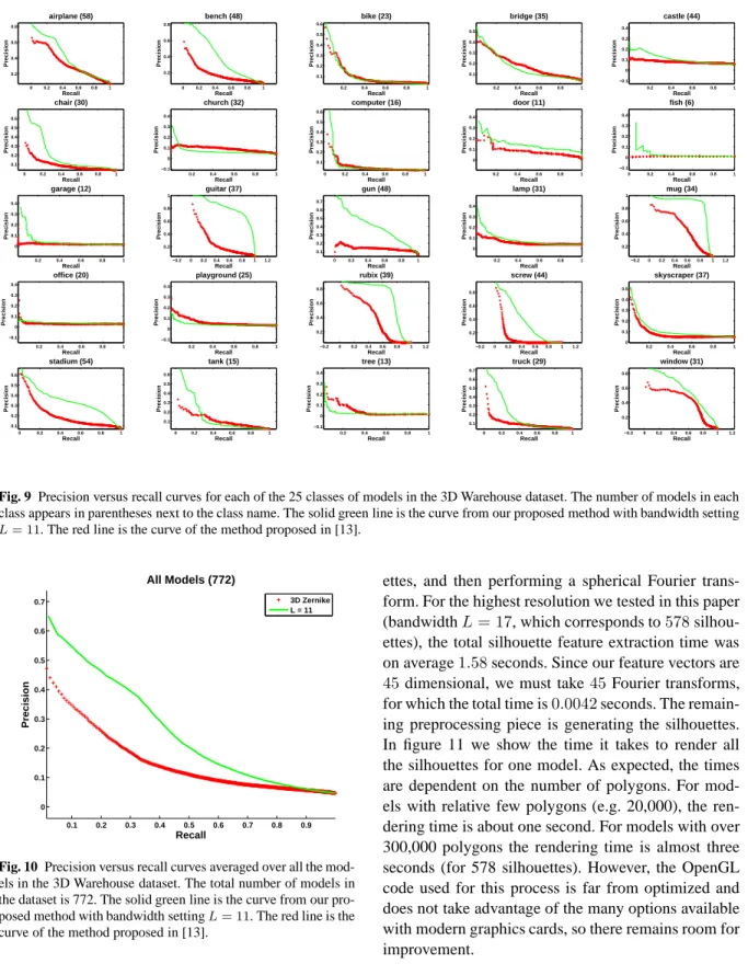
Fig. 9 Precision versus recall curves for each of the 25 classes of models in the 3D Warehouse dataset. The number of models in each

class appears in parentheses next to the class name. The solid green line is the curve from our proposed method with bandwidth setting

L= 11. The red line is the curve of the method proposed in [13].

0.1 0.2 0.3 0.4 0.5 0.6 0.7 0.8 0.9 0 0.1 0.2 0.3 0.4 0.5 0.6 0.7 Recall Precision All Models (772) 3D Zernike L = 11

Fig. 10 Precision versus recall curves averaged over all the

mod-els in the 3D Warehouse dataset. The total number of modmod-els in the dataset is 772. The solid green line is the curve from our pro-posed method with bandwidth settingL= 11. The red line is the curve of the method proposed in [13].

ation, but the computation time is still important since the query models may not have been seen before. In our algorithm feature generation involves generating model silhouettes, extracting features from the

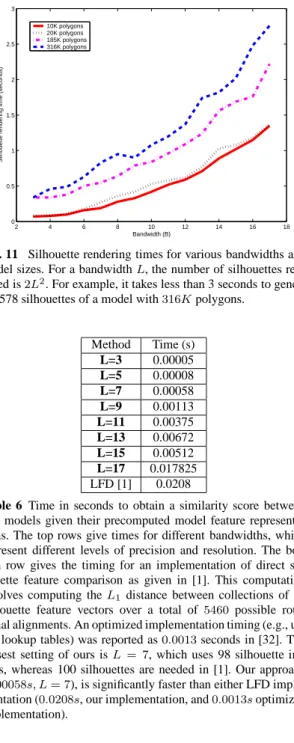
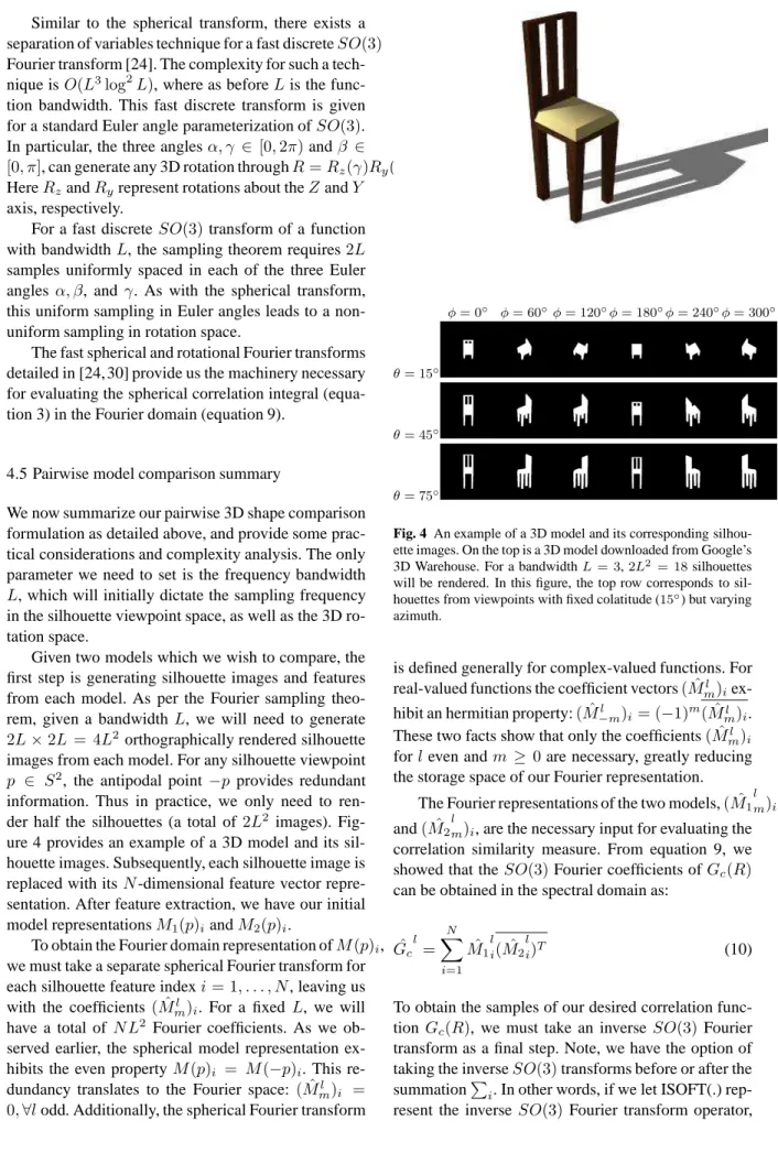
silhou-ettes, and then performing a spherical Fourier trans-form. For the highest resolution we tested in this paper (bandwidthL= 17, which corresponds to578 silhou-ettes), the total silhouette feature extraction time was on average1.58seconds. Since our feature vectors are 45dimensional, we must take45Fourier transforms, for which the total time is0.0042seconds. The remain-ing preprocessremain-ing piece is generatremain-ing the silhouettes. In figure 11 we show the time it takes to render all the silhouettes for one model. As expected, the times are dependent on the number of polygons. For mod-els with relative few polygons (e.g. 20,000), the ren-dering time is about one second. For models with over 300,000 polygons the rendering time is almost three seconds (for 578 silhouettes). However, the OpenGL code used for this process is far from optimized and does not take advantage of the many options available with modern graphics cards, so there remains room for improvement.

The online cost of the model comparison algorithm is the computation time required to estimate the corre-lation functionGc(R)and identify the maximum value.

Timings for evaluating equation 12 at various band-width settings, as well as a comparison with [1], are

2 4 6 8 10 12 14 16 18 0 0.5 1 1.5 2 2.5 3 Bandwidth (B)

Silhouette rendering time (seconds)

10K polygons 20K polygons 185K polygons 316K polygons

Fig. 11 Silhouette rendering times for various bandwidths and

model sizes. For a bandwidthL, the number of silhouettes ren-dered is2L2_{. For example, it takes less than 3 seconds to}

gener-ate 578 silhouettes of a model with316Kpolygons.

Method Time (s) L=3 0.00005 L=5 0.00008 L=7 0.00058 L=9 0.00113 L=11 0.00375 L=13 0.00672 L=15 0.00512 L=17 0.017825 LFD [1] 0.0208

Table 6 Time in seconds to obtain a similarity score between

two models given their precomputed model feature representa-tions. The top rows give times for different bandwidths, which represent different levels of precision and resolution. The bot-tom row gives the timing for an implementation of direct sil-houette feature comparison as given in [1]. This computation involves computing theL1 distance between collections of10

silhouette feature vectors over a total of 5460 possible rota-tional alignments. An optimized implementation timing (e.g., us-ing lookup tables) was reported as0.0013seconds in [32]. The closest setting of ours isL = 7, which uses 98 silhouette im-ages, whereas 100 silhouettes are needed in [1]. Our approach (0.00058s, L= 7), is significantly faster than either LFD imple-mentation (0.0208s, our implementation, and0.0013soptimized implementation).

given in table 6. The machine used to generate these timings is a Apple Powerbook laptop computer with 2GB of RAM.

8 Conclusion

In this paper we presented a new similarity measure for comparing 3D shapes based on a visual representation, as well as a novel estimation technique for the efficient evaluation of the similarity measure. We showed how an analysis in the spherical Fourier domain provides a flexibility to all components of our formulation, and

can also lead to a very intuitive and effective coarse-to-fine 3D model retrieval system.

A thorough evaluation on multiple benchmarks shows our proposed methods combine the discriminative power of a visual model representation with efficient compu-tation.

8.1 Acknowledgments

We thank Corey Goldfeder for the implementation of the 3D Zernike descriptors described in [13].

References

1. D.-Y. Chen X.-P. Tian, Y.T.S., Ouhyoung, M.: On visual similarity based 3D model retrieval. In: Eurographics (2003)

2. Kazhdan, M., Funkhouser, T., Rusinkiewicz, S.: Rotation in-variant spherical harmonic representation of 3D shape de-scriptors. In: Symposium on Geometry Processing (2003) 3. Vranic, D.V.: An improvement of rotation invariant 3D

shape descriptor based on functions on concentric spheres. In: Proceedings of International Conference on Image Pro-cessing, pp. 757–760 (2003)

4. Saupe, D., Vranic, D.V.: 3D model retrieval with spheri-cal harmonics and moments. In: Proceedings of the 23rd DAGM-Symposium on Pattern Recognition, pp. 392–397. Springer-Verlag, London, UK (2001)

5. Ankerst, M., Kastenm¨uller, G., Kriegel, H.P., Seidl, T.: Nearest neighbor classification in 3D protein databases. In: Proceedings of the Seventh International Conference on In-telligent Systems for Molecular Biology, pp. 34–43. AAAI Press (1999)

6. Kang, S.B., Ikeuchi, K.: Determining 3-D object pose using the complex extended gaussian image. In: Proceedings of the 1991 IEEE Computer Society Conference on Computer Vision and Pattern Recognition (CVPR ’91) (1991) 7. Horn, B.K.P.: Extended gaussian images. IEEE 72, 1671–

1686 (1984)

8. Osada, R., Funkhouser, T., Chazelle, B., Dobkin, D.: Match-ing 3D models with shape distributions. In: SMI ’01: Pro-ceedings of the International Conference on Shape Model-ing & Applications, pp. 154–166. IEEE Computer Society, Washington, DC, USA (2001)

9. Ohbuchi, R., Osada, K., Furuya, T., Banno, T.: Salient lo-cal visual features for shape-based 3D model retrieval. In: IEEE International Conference on Shape Modeling & Ap-plications (2008)

10. Ohbuchi, R., Minamitani, T., Takei, T.: Shape-similarity search of 3D models by using enhanced shape functions. In: TPCG ’03: Proceedings of the Theory and Practice of Com-puter Graphics, p. 97. IEEE ComCom-puter Society, Washington, DC, USA (2003)

11. Tangelder, J.W., Veltkamp, R.C.: A survey of content based 3d shape retrieval methods. Multimedia Tools Appl. 39(3), 441–471 (2008)

12. Makadia, A., Visontai, M., Daniilidis, K.: Harmonic silhou-ette matching for 3D models. In: 3DTV. Kos (2007) 13. Novotni, M., Klein, R.: 3D zernike descriptors for content

based shape retrieval. In: SM ’03: Proceedings of the eighth ACM symposium on Solid modeling and applications, pp. 216–225. ACM, New York, NY, USA (2003). DOI http: //doi.acm.org/10.1145/781606.781639

14. Johnson, A.E., Hebert, M.: Using spin images for efficient object recognition in cluttered 3D scenes. IEEE Trans. Pat-tern Anal. Mach. Intell. 21(5), 433–449 (1999)

15. Johnson, A.: Spin-images: A representation for 3-D surface matching. Ph.D. thesis, Robotics Institute, Carnegie Mellon University, Pittsburgh, PA (1997)

16. Frome, A., Huber, D., Kolluri, R., Bulow, T., Malik, J.: Rec-ognizing objects in range data using regional point descrip-tors. In: Proceedings of the European Conference on Com-puter Vision (ECCV) (2004)

17. Kortgen, M., Park, G.J., Novotni, M., Klein, R.: 3D shape matching with 3D shape contexts. In the 7th Central Euro-pean Seminar on Computer Graphics (2003)

18. Belongie, S., Malik, J., Puzicha, J.: Shape matching and ob-ject recognition using shape contexts. Pattern Analysis and Machine Intelligence, IEEE Transactions on 24(4), 509–522 (2002)

19. Lowe, D.G.: Object recognition from local scale-invariant features. In: ICCV ’99: Proceedings of the International Conference on Computer Vision-Volume 2, p. 1150. IEEE Computer Society, Washington, DC, USA (1999)

20. Funkhouser, T., Min, P., Kazhdan, M., Chen, J., Halderman, A., Dobkin, D., Jacobs, D.: A search engine for 3D models. ACM Transactions on Graphics 22(1), 83–105 (2003) 21. Thurston, W.P.: Three-Dimensional Geometry and

Topol-ogy. Princeton University Press (1997)

22. Zhang, D.S., Lu, G.: An integrated approach to shape based image retrieval. In: Proc. of 5th Asian Conference on Com-puter Vision (ACCV), pp. 652–657. Melbourne (2002) 23. Burel, G., Henoco, H.: Determination of the orientation of

3D objects using spherical harmonics. Graph. Models Im-age Process. 57(5), 400–408 (1995)

24. Kostelec, P.J., Rockmore, D.N.: FFTs on the rotation group. In: Working Paper Series, Santa Fe Institute (2003) 25. Makadia, A., Daniilidis, K.: Rotation recovery from

spher-ical images without correspondences. IEEE Trans. Pattern Anal. Mach. Intell. 28(7), 1170–1175 (2006)

26. Kazhdan, M.: An approximate and efficient method for op-timal rotation alignment of 3D models. IEEE Trans. Pat-tern Anal. Mach. Intell. 29(7), 1221–1229 (2007). DOI http://dx.doi.org/10.1109/TPAMI.2007.1032

27. Kovacs, J.A., Wriggers, W.: Fast rotational matching. Bio-logical Crystallography 58, 1282–1286 (2002)

28. Makadia, A., Sorgi, L., Daniilidis, K.: Rotation estima-tion from spherical images. In: ICPR ’04: Proceedings of the Pattern Recognition, 17th International Conference on (ICPR’04) Volume 3, pp. 590–593. IEEE Computer Soci-ety, Washington, DC, USA (2004)

29. Arfken, G., Weber, H.: Mathematical Methods for Physi-cists. Academic Press (1966)

30. Driscoll, J., Healy, D.: Computing fourier transforms and convolutions on the 2-sphere. Advances in Applied Mathe-matics 15, 202–250 (1994)

31. Makadia, A., Daniilidis, K.: Direct 3D-rotation estimation from spherical images via a generalized shift theorem. In: IEEE Conf. Computer Vision and Pattern Recognition. Wis-consin, June 16-22 (2003)

32. Shilane, P., Min, P., Kazhdan, M., Funkhouser, T.: The princeton shape benchmark. In: Shape Modeling Interna-tional. Genova, Italy (2004)

33. AIM@SHAPE: http://give-lab.cs.uu.nl/

shrec/shrec2006/(2006)

34. Typke, R., Veltkamp, R.C., Wiering, F.: Evaluating retrieval techniques based on partially ordered ground truth lists. In: Proceedings International Conference on Multimedia & Expo (2006)

35. Veltkamp, R.C., Ruijsenaars, R., Spagnuolo, M., van Zwol, R., ter Haar, F.: Shrec2006 3d shape retrieval contest. tech-nical report, Utrecht University (2006)