DiSTA
Dipartimento di Scienze Teoriche e Applicate
P H D T H E S I S
to obtain the title ofPhD of Science
Specialty : Computer Science
Defended by
C ¨
UNEYT G ¨
URCAN
AKC
¸ ORA
PROFILING USER
INTERACTIONS ON ONLINE
SOCIAL NETWORKS
Advisor: Barbara
Carminati
Advisor: Elena
Ferrari
defended on January 7, 2013
Jury :
Reviewers : James Joshi - University of Pittsburgh, USA
President : Claudio Gentile - University of Insubria Examinators : ... ... - ...
... ... - ...
... ... - ...
Acknowledgment
I would like to express the deepest gratitude to my advisors Elena Ferrari and Barbara Carminati. In addition to their academic guidance, they have shown a great deal of pa-tience towards me and supported my research in a way that goes beyond a professional relationship. Their caring attitude has always given me the strength to continue my re-search endeavor.
I would like to thank William Lucia for his work with me in hist last year in Master’s degree.
My lab partners Lorenzo Bossi, Dr. Stefano Braghin, Dr. Paolo Brivio, Michele Guglielmi, Lui Geng and Dr. Pietro Colombo have contributed to my research in dis-cussions, shown me the Italian hospitality and enriched my life greatly. Without them, my Ph.D would never be such a great experience.
I have spent many enjoyable moments with professors Alberto Trombetta, Claudio Gentile, Marco Tarini, Paolo Massazza and Mauro Ferrari. I would like to thank them for their kindness.
I would like to thank Mauro Santabarbara for his time in helping me with servers and computers that I used during my research. Not officially, but he has always been my third advisor.
Finally, I would like to thank the Italian people for their warmth and grace, which made me feel at home during these years. Your country is a heaven, not only because of your lakes, mountains and valleys, but also because of your cultured life, tolerance and kindness.
Abstract
Over the last couple of years, there has been significant research effort in mining user behavior on online social networks for applications ranging from sentiment analysis to marketing. In most of those applications, usually a snapshot of user attributes or user relationships are analyzed to build the data mining models, without considering how user attributes and user relationships can be utilized together.
In this thesis, we will describe how user relationships within a social network can be further augmented by information gathered from user generated texts to analyze large scale dynamics of social networks. Specifically, we aim at explaining social network interactions by using information gleaned from friendships, profiles, and status posts of users. Our approach profiles user interactions in terms of shared similarities among users, and applies the gained knowledge to help users in understanding the inherent reasons, consequences and benefits of interacting with other social network users.
Contents
1 Introduction 12
1.0.1 Outline of the Dissertation . . . 14
2 Related Work 16 2.1 Introduction . . . 16
2.2 Similarity metrics . . . 16
2.2.1 Network Similarity . . . 18
2.2.2 Profile Similarity . . . 22
2.3 Privacy in user interactions . . . 23
2.4 Risk in user interactions . . . 25
2.5 Detecting Anomalies in Interactions . . . 27
2.6 Micro analysis of Interactions . . . 27
3 User Similarity and Interactions 29 3.1 Introduction . . . 29
3.2 Similarity Measures . . . 30
3.2.1 Network Similarity . . . 30
3.2.2 Profile Similarity . . . 32
3.3 Experimental Methodology . . . 38
3.4 Experimental Results on Undirected Graphs . . . 42
3.4.1 Comparison of Network Similarity Measures . . . 42
3.4.2 Comparison of Profile Similarity Measures . . . 43
3.4.3 Inferrals in Item Similarity . . . 44
3.4.4 Combining Network and Profile similarity . . . 47
3.5 Experimental Results on Directed Graphs . . . 48
3.5.1 Comparison on Network Similarity Measures . . . 48
3.5.2 Comparison of Profile Similarity Measures on Directed Graphs . . . 55
3.6 Absolute Performance Values . . . 56
3.6.1 Profile Similarity . . . 56
3.6.2 Network Similarity . . . 58
3.7 Discussion on Experimental Results . . . 61
3.8 Conclusion . . . 62
4 Explaining Privacy with Interactions 64
4.1 Introduction . . . 64
4.2 How to measure risk . . . 66
4.3 Risk Learning Process . . . 68
4.3.1 Risk Labels . . . 69
4.3.2 Stranger sampling . . . 69
4.3.3 Classifier . . . 71
4.3.4 Termination . . . 73
4.4 Experiments on Facebook data . . . 74
4.4.1 Facebook Dataset . . . 75
4.4.2 Parameters setting . . . 76
4.4.3 Risk learning process . . . 76
4.4.4 Risk Measure . . . 77 4.5 Conclusions . . . 81 5 Risks of Interactions 83 5.1 Introduction . . . 83 5.2 Overall Approach . . . 84 5.3 Transforming Data . . . 85 5.3.1 Clustering Friends . . . 86 5.3.2 Clustering Strangers . . . 87 5.3.3 Clustering Algorithms . . . 88 5.4 Baseline Estimation . . . 88 5.5 Friend Impact . . . 90
5.5.1 The Past Labeling Parameter . . . 91
5.5.2 The Friend Impact Parameter . . . 92
5.6 Friend Risk Labels . . . 93
5.7 Experimental Results . . . 94
5.7.1 Validating Model Assumptions . . . 94
5.7.2 Training for Baseline . . . 94
5.7.3 Clustering . . . 96
5.7.4 Friend Impacts and Risk Labels . . . 100
5.8 Conclusion . . . 101
6 Detecting Anomalies in Interactions 102 6.1 Introduction . . . 102
6.2 Overview of the Problem . . . 103
6.3 Methodology . . . 105
6.3.1 Topic Models . . . 105
6.3.2 Clusters . . . 106
6.3.3 Anomaly Definitions . . . 106
6.4 Experimental Analysis . . . 108
6.4.2 LDA Results for Topics . . . 108
6.4.3 Network Data and Changing Data Interests . . . 110
6.4.4 Anomaly Results . . . 111
6.4.5 Validation of Anomalies . . . 116
6.5 Experimental Discussion . . . 119
6.6 Conclusions . . . 122
7 Micro Analysis of User Interactions 123 7.1 Introduction . . . 123
7.2 Data collection . . . 124
7.3 Methodology and tools . . . 125
7.4 Mining Dimensions . . . 125
7.4.1 Entity Recognition . . . 126
7.4.2 Sentiment Analysis . . . 127
7.4.3 Lexical Analysis . . . 129
7.5 Dimension interplay . . . 130
7.6 Influence of Geolocation on Conversations . . . 132
List of Figures
3.1 An exemplary social graph for a target useru. Six friends and two strangers are shown in the graph as nodes, and their friendship relations are denoted
by edges. . . 32
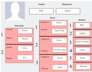
3.2 An exemplary profile for target useru. The profile consists of single valued gender and hometown items, as well as multiple valued education and work items. . . 35
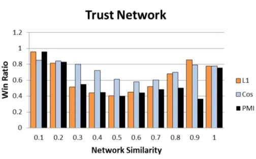
3.3 Win ratio against L1, Cosine, and PMI. The x-axis shows increasing network similarity values. . . 43
3.4 Win/loss ratios for [0.3,0.7] similarity range . . . 43
3.5 Percentage of missing item values for the considered dataset. . . 45
3.6 The effect of network and profile similarity for new edge creation. . . 46
3.7 Graph creation process in Youtube dataset. . . 48
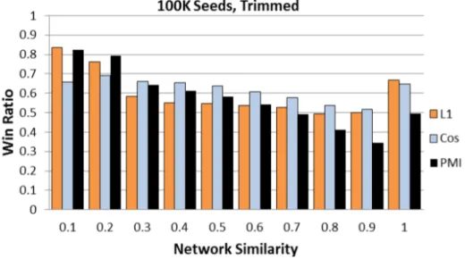
3.8 Win ratios of NS against the other similarity measures for 100K seed nodes in a trimmed network. . . 50
3.9 Win ratios of NS against the other similarity measures for 100K seed nodes in an untrimmed network . . . 51
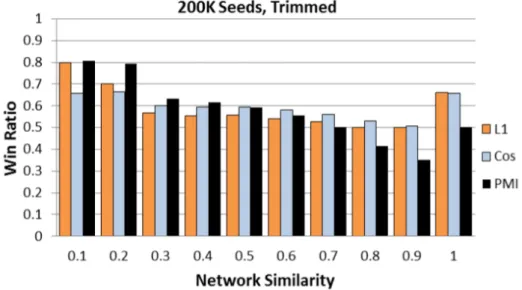
3.10 Win ratios of NS against the other similarity measures for 200K seed nodes in a trimmed network . . . 52
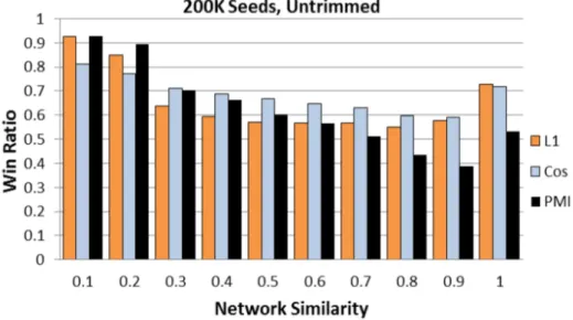
3.11 Win ratios of NS against the other similarity measures for 200K seed nodes in an untrimmed network . . . 53
3.12 Trust, distrust and mixed relations on the graph. Dashed edges are the predictions. . . 53
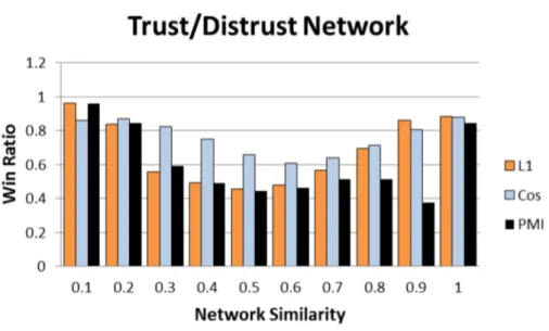
3.13 Win ratios of NS against other similarity measures for Epinions distrust network. X-axis values are increasing NS values . . . 54
3.14 Win ratios of NS against other similarity measures for Epinions trust network 54 3.15 Win ratios of NS against other similarity measures for combined Epinions network . . . 55
3.16 Figure shows average profile similarity as time progresses. The x-axis values are number of months since a user first rated another Epinions user. . . 56
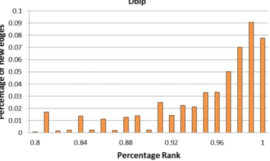
3.17 Percentage of strangers of newly formed edges on the DBLP dataset by their ranks according to NS. . . 59
3.18 Percentage of strangers of newly formed edges on the Facebook dataset by
their ranks according to NS. . . 59
3.19 Percentage of strangers of newly formed edges on the Youtube dataset by their ranks according to NS. . . 60
3.20 Percentage of strangers of newly formed edges on the Epinions dataset by their ranks according to NS. . . 61
4.1 Risk learning process . . . 69
4.2 Network and profile based pools . . . 72
4.3 Snapshot from the extension . . . 75
4.4 Stranger count for network similarity groups . . . 77
4.5 Error rate by rounds for NPP and NSP pools. . . 78
4.6 Average number of unstabilized labels for NPP and NSP pools. . . 78
4.7 Percentage of very risky strangers in network similarity groups . . . 79
5.1 Features and risk labels . . . 89
5.2 Friend impact definitions by considering the number of friends from the same cluster. In the single impact definition, two friends do not increase the friend impact. . . 92
5.3 Deviation of user given labels from baseline labels. Values in the x-axis are the number of mutual friends between a stranger and user. . . 96
5.4 Coefficient of determination (R2) values for 2 and 9 friend clusters . . . 97
5.5 Coefficient of determination (R2) values for 5, 6 and 7 friend clusters . . . . 98
5.6 Coefficient of determination (R2) values of friend impacts for 158 and 8 stranger clusters. . . 98
5.7 Coefficient of determination (R2) values of friend impacts for 26 and 49 stranger clusters . . . 99
5.8 Percentage of positive and negative impact values for friend clusters. . . 100
6.1 Old and new friends of users . . . 104
6.2 Topics and their top words. . . 109
6.3 Changing friend counts on the Twitter network. The x-axis values are num-bers of friends in 2009. In the y-axis, median values of 2013 friend counts are shown. As shown in the left bottom corner of the chart, Twitter users who had almost zero friends in 2009 have a median number of 150 friends in 2013. X-axis values are limited to a maximum of 750 for a better viewing experience. . . 111
6.4 Number of friendships among users of different tweetLDA topics. . . 112
6.5 Similarity of newly added friends to old friends with bioLDA used as the topic model to define profile vectors. . . 113
6.6 Similarity of newly added friends to old friends with tweetLDA used as the topic model to define profile vectors. . . 113
6.7 Similarity of deleted friends to old friends with bioLDA used as the topic
model to define profile vectors. . . 114
6.8 Similarity of deleted friends to old friends with tweetLDA used as the topic model to define profile vectors. . . 115
6.9 The relationship between number of collective anomaly friends and number of old friends for ξ = 0.6 and ξ = 0.7. An increasing ξ value results in a bigger number of anomalous friends. . . 117
6.10 Wordclouds of explanations for validator given decisions to the friendships which were detected as anomalies by our methods. . . 119
7.1 Entities and their percentage in Facebook and Twitter posts. . . 126
7.2 Most frequently mentioned organizations on Facebook. . . 127
7.3 Percentage of sentiments in Facebook and Twitter posts. . . 128
7.4 Most frequently mentioned organizations on Twitter. . . 129
7.5 The impact of sentiments on like and retweet counts. . . 129
7.6 Lexical errors on social networks. . . 131
7.7 Average lexical errors by sentiments in Facebook and Twitter posts. . . 131
7.8 Lexical errors and interactions. . . 133
7.9 Locations of Twitter users. Edges show retweet behavior among Twitter users.133 7.10 In miles, distances between user pairs who retweet each other’s tweets. . . 134
7.11 Like interactions among Facebook users of different locales. . . 135
8.1 Help Interface 1 . . . 148
8.2 Help Interface 2 . . . 148
8.3 Training Interface . . . 149
List of Tables
2.1 Network Similarity Metrics . . . 19
3.1 Education items of a stranger (x) and a target user (u). Number of oc-currences of item values on profiles of u’s friends are given in parentheses. These values in parantheses are what we termed as the dataset, and they are used to find the similarity between two non-identical item values. . . 37
3.2 Similarity values for identical and non-identical item values for different cat-egorical similarity measures. Assigning 0 implies that there is no similarity between two item values. The highest similarity value is 1, and it is assigned to indicate maximum similarity. By possible, we mean that a specific fre-quency distribution of values in the dataset can result in a 0 or 1 similarity. In computation with multiple item value pairs, an overall similarity value is computed by simple averaging, or by using the similarity value of each pair in a function. . . 40
3.3 Similarity values of three strangers for corresponding categorical similarity measures. . . 41
3.4 Comparison of win/loss/draw counts . . . 42
3.5 Comparison of profile similarity measures. Higher ranks show better per-formance, and the zero similarity column shows the percentage of strangers that are assigned zero similarity. . . 44
3.6 Inferral results . . . 45
3.7 Number of future friends found in depth 2. Trimmed graphs contain fewer future friends than untrimmed ones . . . 51
3.8 Profile similarity rankings for strangers of newly formed friendship edges on Facebook and DBLP datasets. . . 57
3.9 Profile similarity rankings for strangers of newly formed friendship edges on the Epinions dataset. . . 57
4.1 Profile attributes importance . . . 80
4.2 Mined importance of benefits . . . 80
4.3 Owner given θweights . . . 81
4.4 Item visibility for different genders . . . 81
4.5 Visibility of profile items for different locale strangers . . . 82
5.1 Regression results for all data points. p-value=2.22e-16. Total N=4013. . . 95
5.2 Regression results for the first group data points. p-value = 5.6701e-11. Total
N=1520. . . 95
5.3 Performance values for different numbers of stranger clusters. . . 99
6.1 Top words from each one of the top-5 topics of U.S. senators found by tweetLDA and bioLDA . . . 110 6.2 Percentages of users and friendships that were labeled as anomalous for
different ξ values. . . 115 6.3 Most frequent explanations for false positive anomalies. . . 120 6.4 Most frequent explanations for true positive anomalies. . . 121
7.1 Dimensional statistics and counts of English texts. Entitity, error and sen-timent values are given in percentages. . . 126 7.2 Examples of Facebook posts with sentiments. . . 128 7.3 Examples of tweets with sentiments. . . 130 7.4 Precision and recall values for Twitter and Facebook sentiments. + and
-signs refer to positive and negative sentiments, whereas P. and R. refer to precision and recall, respectively. . . 130 7.5 Examples of Facebook posts with sentiments containing errors. . . 132 7.6 Examples of tweets with sentiments containing errors. . . 132
Introduction
Almost half a century has passed since the ARPANET network crashed when for the first time researchers attempted to transmit a word from a workstation at University of California to another one at the Stanford Research Institute. What started as a government funded defense project with the ARPANET has in years evolved into a huge network that carries and supports resources and services, such as personal blogs, news media sites, social networks, video sharing sites and online gaming platforms.
In the early days of the Internet, although work stations could communicate with each other, ordinary users were still out of the picture as the Internet was limited to commu-nications among universities and research centres. Starting with the 90s, the Internet saw the creation of hyper-text documents and the World Wide Web, which connected these documents. Web browsers, such as the Netscape Navigator, were developed to surf the WWW, and scripting languages, such as JavaScript, were created to provide interactive hyper-text documents.
Despite interactive elements, the first hyper-text documents were static in the sense that they were loaded into the web browsers as “static screenfuls”.1 In 1999, the Web 2.0 concept was pushed forward to open web sites and documents to ordinary user input, and allow users to create, mesh and change documents. The Web 2.0 concept advanced the idea that user created content could replace or augment static web pages, and web sites could benefit from user collaborations. Although some services existed before the concept, with Web 2.0, online social networks, personal blogs, collaboration wikis, and video sharing services grew more popular.
While these fundamental changes were happening on how the Internet was being used, research works have been looking into network communications, and finding global patterns that explain dynamics within the Internet topology [44, 27, 132]. Once the WWW came into existence, research works turned their attention to human communications, and found that the Internet communication patterns, to some degree, also applied to human interactions. For example, the power law theory [44] that has originated from works on the Internet topology has also been observed on social networks [96].
1
Excerpted from Fragmented Future by Darcy DiNucci.
Increased attention to human interactions has also benefited from a growing number of online human population. Web 2.0 influenced services, such as social networks, personal blogs and even video sharing services, have become very popular in recent years and at-tracted a huge registered user base. Among these, online social networks hold the most data about the Internet users; starting with the SixDegrees.com in 1997, online social net-works, such as Friendster in 2002 and Facebook in 2004, became popular among hundreds of millions of users.
The growing population of online social network users has resulted in an abundance of user generated data, whether of the new friendships users make or profile information they enter. Social networks have also developed new functionalities such as “likes” and “shares” on Facebook, that increase the number of user generated data items (i.e., traces or texts of user involvement on the social network). From an information retrieval point of view, regardless of the studied social network, users’ friendships, or connections to other social network users are the easiest data items to retrieve and analyze. A connection is also easy to represent on a global graph; the two users are denoted as two nodes, and the connection becomes the edge between them. By considering all friendships, a global graph can be constructed, and problems, such as influence propagation [66] or user clustering [78], can be studied with techniques that have been developed in graph theory works [103].
A specific problem that hindered efforts to utilize user generated text data, such as profile information or status posts, is that these data items were unstructured or noisy. For example, user locations on Twitter are still manually typed, therefore unstructured, because users do not have to choose their city, region, country values from a list. For this reason, aggregating user locations from many Twitter users are difficult and time consuming. Despite these problems, several research works have utilized user generated text and profile data. For example, the influence of gender and race/ethnicity of users have been studied to understand network behavior [79] on Facebook, and Twitter users have been modeled to provide personalized news services [1]. However, difficulties in aggregating text based user data has hindered efforts to combine network information (e.g., friendships) with text based information (e.g., users’ posts and bios).
In recent years, the unstructured user data problem has been alleviated by the choice of online social network companies to provide an API access to their social network data. For their APIs, online social network companies have created structured user profiles. For example, Facebook has transitioned to a structured version of its user profiles by accepting most frequent manually entered data values as its predefined data values. A further data standardizing effort on social networks has resulted in a machine readable ontology in FOAF (Friend of a Friend) [51]. With FOAF, social network users and their relations to each other can be described in attributes within and across different social networks.
Our work shares a common goal with the FOAF approach; once the edges in a social network graph are labeled with shared attributes, or users are profiled with their attributes, a large scale analysis of shared attributes and created edges can be completed to have a better understanding of why and how interactions happen among social network users. Such an analysis can be used to understand and verify the sociological theories. Specifically we focus on the homophily [92] and heterophily [113] theories from sociology.
According to homophily, personal attributes and connections affect creation of new ties in social life and result in homogeneous groups of individuals. Political party supporters and religious communities are examples of homophilous groups. In contrast to homophily, heterophily is the tendency to interact with people that are not similar to you. In social networks, this tendency is mainly motivated by the fact that social interactions (e.g., creation of new relationships) might give a user some benefits in terms of acquaintance of new information.
In this thesis, we will describe how network connections within a social network can be further augmented by information gathered from user generated texts to analyze large scale dynamics of social networks. Specifically, we aim at explaining social network interactions by using information gleaned from friendships, profiles, and status posts of users. Our approach profiles user interactions in terms of shared similarities among users, and applies the gained knowledge to help users in understanding the inherent reasons, consequences and benefits of interacting with other social network users.
1.0.1 Outline of the Dissertation
The content of this dissertation is described in the following:
Related Work
In the related work chapter, we will explain previous work on finding similarities of users, and give the related work which deal with user interactions in privacy and risk domains. Afterwards, we will outline existing work in detecting which interactions among social network users can be labeled as anomalies. The chapter closes with the related work on micro analysis of user generated data to explain interactions. The content of this chapter is based on “Graphical User Interfaces for Privacy Settings” [10] and “Similarity Metrics on Social Networks” [11].
User Similarity in Interactions
In this chapter, we build on current research and propose measures for evaluating social network users’ similarity according to both their connections and profile attributes. From the network connections perspective, we propose a novel measure that facilitates finding user similarity without observing an important fraction of the network. This approach reduces computational costs by limiting the number of queries to be performed on the network. We also propose a profile similarity measure to find semantic similarities among users. Moreover, since user profile data could be missing, we present a technique to infer them from profile items of a user’s contacts. Metrics that are studied in this chapter constitute the building block of our studies in the following chapters. The results presented in this chapter has been published in [9].
Explaining Privacy with Interactions
In this chapter, we focus on the risk of new interactions from a privacy point of view. We investigate a risk measure to help users in judging another user with whom they might create a friendship relation. We assume that risks of interactions are impacted by several different dimensions, such as the other user’s characteristics and shared friends, whose importance may greatly vary from user to user. Our risk measure captures the personal judgment of users, and helps them in forming their own opinions. This study has been tested with real life social network data through a human experiment, and the results validate our approach. The results presented in this chapter has been published in [7].
Risks of Interactions
Once we have learned privacy decisions of users in Chapter 4, we turn our attention to labeling users’ interactions with their one and two degree neighbors on the social network. Based on neighbors’ characteristics, in this chapter we categorize social network users, and find that all neighbors can be put into a relatively small number of groups, regardless of their differing characteristics. The results presented in this chapter has been published in [8].
Detecting Anomalies in Interactions
In this chapter, we propose novel anomaly detection measures that use both categories of users and the evolution of the social network graph. Our proposed anomaly measures model a user based on his/her social network structure and the characteristics of the other users she/he follows on the network. In this study we consider the follower relationship on Twitter as an interaction which is initiated to benefit from learning about another user’s tweets. Through a large user experiment, we empirically show that anomalies in interactions can be found by analyzing data consumption patterns in a social network graph. The results presented in this chapter has been published in [64].
Micro Analysis of User Interactions
In this chapter, we study the problem of how interactions are governed by certain charac-teristics of posts across Facebook and Twitter. Rather than external features such as the network structure or user information, we focus on tweets/posts themselves to understand what aspects of tweets/posts help them to get retweeted and liked. Moreover, we analyze how location information influences retweet, comment and like interactions. The results presented in this chapter has been published in [85].
Related Work
2.1
Introduction
With the increasing popularity of online social networks, many studies have been carried on to better understand how and why humans interact on social networks (see e.g., [42, 131]). As our research has focused on using both the network information and the user generated data, we will start discussing the related work that have focused on finding and explaining commonalities between users with similarity metrics. Afterwards, we will give the state of art in profiling user interactions from privacy, risk and anomaly perspectives. We conclude this chapter with the related work which explain user interactions with certain dimensions of user generated data, such as the sentiments expressed in user posts.
2.2
Similarity metrics
In the literature, the term similarity has been used in different meanings (e.g., the short distance between two users, shared features or shared actions) to quantize similarity for different application fields. Some work have attempted to define similarity rigorously [112, 54, 81]. Among these, the four principles by Lin [81] are widely used to implement similarity metrics on social networks. We will explain these four principles with commonal-ity, differences, maximum and minimum similarity. Incommonality, shared commonalities (e.g., race, gender, sex of users) increase the similarity of two users. On the other hand, the more differences lead to smaller similarity. Regardless of the number of features, two users are said to have the maximum similarity when they are identical in every feature. Similarly, regardless of the number of features, two users are the least similar when they are different in every feature. In current studies, the maximum and minimum similarity values are given as 0 and 1, respectively.
A more rigorous set of properties for similarity metrics can be adopted from distance metrics by considering similarity = 1−distance. For any given distance metric, these properties are 1) symmetry, 2) identity, 3) non-negativity, and the 4) triangle equality. In the identity property, distance(a, b) = 0, when a = b. On social networks this property
can have different explanations; on the graph structure distance(a, b) = 0 is assumed to be true when the two nodes have the same set of friends, whereas if profile information are considered, two users must have the same values for every profile item. In setting a lower bound for distance, the non-negativity property defines distance(x, y) ≥ 0 for any user pair. The symmetry condition assures that distance(a, b) = distance(b, a), while in the triangle equality distance(a, c)≤distance(a, b) +distance(b, c).
The absence of some of these properties can be used to classify different formulas. For example, quasi-metrics do not provide the symmetry property, whereas semi-metrics do not have the triangle property. Traditionally, the symmetry property is not applicable in directed networks, because directions of edges can lead to different similarity values for a pair of users. In this case, two different values are computed; sim(a, b) denotes the similarity value according to a user a and sim(b, a) denotes a potentially different value from the perspective of user b.
Similarly, the triangle equality is difficult to achieve for similarity of user profiles because profiles can consist of more than one dimension (i.e., profile item). As a result, although the triangle property holds for one dimension, similarities for three user profiles with multiple dimensions might not adhere to the triangle property. Ideally, any formula that does not carry all these four properties should be called a measure, but researchers still prefer to use the word metric interchangeably with the term measure.
Founded upon these theoretical definitions, similarity metrics that have been proved efficient and practical on social networks are those that exploit a locality principle in similarity computations. The basic idea underlying such metrics is that, given two social network users, their similarity is computed by observing only a subset of vertices (e.g., friends of the two users) in the social network. This approach restricts required information about the social network to a minimum, and reduces the required time of calculations. Even though global measures (e.g., the shortest path between users, or the community membership of users) can be used in the same context, they are more costly in time and computational power because they require too much information about the social network. For example, shortest path calculation might require observing friendship links of many users. Moreover, even though the costs can be undertaken, researchers and companies cannot have access to the whole social network data because of privacy issues. Only owners of social networking services can have the complete data that is required to compute global similarity measures. Therefore, local similarity metrics provide a simple alternative in the face of these costly issues.
In 1970s, early attempts at defining similarity metrics involved finding similarities among text based documents [91] that were modeled as a collection of words. Similar-ity metrics were used to discover relations between documents or rank the documents according to their similarity to a given query. These efforts have resulted in several well known metrics, such as the Cosine and Jaccard similarities [55]. With the advent of the Internet, researchers have applied document based similarity metrics to user generated web items, such as friendships and status posts, to discover relationships between web users. Specifically, similarity research on user generated data has focused on predicting links (relationships) among users and mining past user behavior to predict future actions.
In the link prediction problem [80], similarity of social network users has been exploited to predict new friendships. In this context, high similarity between two social network users is assumed to increase the probability of them creating a new friendship [118]. With generalization, this idea has been explored in the homophily theory which states that people tend to be friends with other people who are similar to them along personal attributes, such as gender, race and religion [92].
In addition to user characteristics, actions of a user is exploited to predict actions of similar users. This idea has been studied in recommender systems to observe existing item ratings (for movies, books, songs etc.) of users and predict ratings of unseen items [93]. Similar users are assumed to give similar ratings to similar items. From this assumption, similarity of ratings are predicted by finding either similar users (i.e., user based) or similar items (i.e., item based).
On social networks, user generated data are classified into two types: profile data, which refers to user entered textual information, such as personal information, and network data, that is information on created relationships, such as friendships with other users on the social network. Depending on the type of user data, similarity metrics differ in how they model a social network user. Furthermore, some similarity metrics can be used only on one type of user generated data. By taking this into account, we will first explain how similarity metrics work on network data, and then continue to explain metrics for profile data.
2.2.1 Network Similarity
In network similarity metrics, existing user relationships are exploited to find similarity. For example, a big number of shared friends between two users can be assumed to imply their high similarity. Network data that represent relationships can be modeled as a graph
G = (V, E), where each user a in the network is considered a vertex va ∈ V, and a
relationship between users aand b is an edgeeab ∈E on the graphG. If relationships are
established by mutual consent of two users, an edge between them is said to be undirected (the edge has no start and end points), and it can be called a friendship. Friendship relations on social networks, such as Facebook, Orkut, and LinkedIn, are modeled with undirected graphs. On an undirected graph, first level neighbors of a vertex va are a set
of vertices Γ(va) who share an edge with va (e.g., friends of a). Similarly, second level
neighbors Γ(Γ(va)) (e.g., friends of friends of a) share an edge with first level neighbors of a. If relationships can be created without mutual consent, an edge is said to be directed; it starts from the user who initiated the relationship (i.e., source vertex) and ends at the user with whom the relationship was established (i.e., target vertex). For example, the popular social networks Twitter and Google+ are directed social networks; when user a
starts following user b, an edge is created, starting from vertex va and ending at vertex vb. On directed graphs, the friendship term from undirected graphs is replaced with
in-neighbors andout-neighbors. In-neighbors Γ−(va) and out-neighbors Γ+(va) of a vertexva
are defined as target and source vertices of all edges that have vertex va as their source
Measure Formula Description
Overlap |Γ(va)∩Γ(vb)| The number of common
neighbors.
Preferential Attachment |Γ(va)| × |Γ(vb)| Multiplied neighbor
counts of both users. Jaccard (|Γ(va)∩Γ(vb)|)/(|Γ(va)∪Γ(vb)|) The percentage of
shared neighbors over all neighbors.
Cosine (|Γ(va)∩Γ(vb)|)/(
p
(|Γ(va)|.|Γ(vb)|)) The number of common
neighbors normalized by multiplied neighbor counts.
Adamic & Adar P
vc∈{Γ(va)∩Γ(vb)} 1
Log(|Γ(vc)|) Common neighbors who
have very few neighbors are given more impor-tance.
Point-wise Mutual Information P(Γ(va),Γ(vb))×log
P(Γ(v
a),Γ(vb))
P(Γ(va)).P(Γ(vb))
How much the prob-ability of having the current set of common neighbors differs from the case where neigh-bors would be added by users on the graph ran-domly.
Katz’s Measure
+∞
P
p=1
βp×N umOf P ath(va, vb, p) Similarity is implied by
the number and length of paths that connect two users on the graph. Each path 0< p <+∞, whereas 0< β <1.
Although the similarity metrics are designed to work with the neighborhood notion of undirected graphs, they can be applied to directed networks by small modifications. For example, direction of edges can be removed to make the graph undirected. Another approach is to consider only one type of edges (out-neighbors or in-neighbors) as neighbors while using the metrics. As these modifications can be used to define neighbors of a user on directed graphs, we will give metric definitions in terms of user neighbors. Assume that a similarity function sim(va, vb) computes the similarity of users va and vb by considering
their neighbors Γ(va) and Γ(vb), respectively. We will denote one of their common neighbors
with vc, i.e., vc ∈ (Γ(va)∩Γ(vb)). High similarity between two users who do not have a
relationship will be assumed to increase the probability of them creating a relationship edge. With these definitions, metric formulas that we will explain are given in Table 2.1. Next we will discuss these network similarity metrics in more details.
Overlap: The overlap measure [124] counts the number of common friends of va and vb to compute similarity.
Preferential Attachment: For relationship creation on social networks, the prefer-ential attachment metric reflects the “rich gets richer” notion from sociology [14]. The metric assumes that highly connected vertices (i.e., users who have many neighbors) are more likely to create relationships with each other.
Jaccard (L1 norm): The Jaccard metric [124] counts the number of common neigh-bors as in the overlap metric, but it normalizes this value by using the total number of neighbors of users va andvb.
Cosine (L2 norm): Cosine similarity was originally devised to find the similarity of two documents by computing the cosine of the angle between their feature vectors [124]. When the angle between the two vectors is 0, they are considered identical, and the cosine of the angle equals the maximum similarity value 1.
Adamic & Adar: Like the overlap metric, Adamic & Adar considers common neigh-bors, but each neighbor’s impact on the similarity value depends on the number of its neighbors [3]. If a common neighbor has few neighbors, its impact on the similarity is assumed to be higher. For example, if usersvaandvb are the only neighbors ofvc, 1/log(2)
is added to the overall similarity. The similarity is computed by summing values from all common neighbors.
Point-wise Mutual Information (Positive correlations): Point-wise mutual in-formation [22] is computed in probabilistic terms where joint probability distribution function P(Γ(va),Γ(vb)) computes the probability of a graph vertex vx ∈ V|x 6= a 6= b
sharing edges with both va and vb, whereas marginal probability distribution functions P(Γ(va)) and P(Γ(vb)) are probabilities of a graph vertex sharing an edge with va and vb, respectively. If edges are assumed to represent friendships, P(Γ(va),Γ(vb)) is equal
to #users in the social network#mutual f riends . Similarly, P(Γ(va)) is equal to #users in the social network#f riends of va . In
other words, point-wise mutual information shows whether two users share mutual friends due to randomness. Note that due to computing probability with the total number of users in the social network, point-wise mutual information produces very low average similarity values, because #users in the social network can be in millions.
vertex on a graph. The vertex which had the biggest number of shortest paths to the other vertices was considered a central vertex with high status. To compute sim(va, vb), Katz’s
measure finds the number of paths that connect vaand vb for path length p, 1< p <+∞.
The number of paths (i.e., the value ofN umOf P ath(va, vb, p)) is dampened by aβp value,
where 0 < β < 1. In practice, the β value is chosen as small as 0.005 [80]. Although p
values can be increased to cover a big portion of the graph, usually p= 2 or p= 3 values are chosen to find similarity, because computations for p > 3 contribute very less to the overall value. Note that although the Katz’s measure can be used as a global measure with big p values, smallp values (e.g., 2 or 3) make it a practical measure for fast, local similarity computations.
In research work, performance of similarity metrics has been compared by making predictions based on similarity values, and validating the results [80, 118]. Typically, metrics are used to predict top-k relationships (e.g., k most probable future friendships that will be created between users) on graphs at a time t1, and these predictions are
validated at a timet2 > t1. The performance of a metric can be computed by counting the
number of correct predictions.
In Liben et al. [80], Adamic & Adar has been shown to perform better than preferential attachment, Jaccard, overlap and Katz’s measure on a scientific co-authorship network. On another social network, Orkut.com, Spertus et al. [118] have found that cosine similarity performed better than Jaccard and point-wise mutual information metrics.
Despite these comparisons, it is important to understand that each metric has its weak-nesses in different application fields. Preferential attachment is widely used in social net-works to predict friendships, but unlike Jaccard or cosine similarity its computed value does not reside within [0,1]. In fact, its max value is only bounded by the total number of users in a social network, because there are no theoretical limits to prevent a user from having every other social network user as a neighbor. However, some social networks may choose to limit the number of neighbors; for example, an undirected network, Facebook, allows up to 5000 neighbors, whereas a directed network, Twitter, does not have such a limit. Because of this, preferential attachment can not be used to quantify how much per-cent two users are similar. When the graph has many vertices (i.e., the probability of an edge between two users are very small), computed value of point-wise mutual information can be very small, and it can not be used to define how muchpercent two users are similar. Point-wise mutual information and preferential attachment can be best used in ranking a set of users according to their similarity to a specific user. There are some limitations in using Katz’s measure too. In popular social networks, discovering edge counts for paths of length 2 or more can be restricted because social networking services do not allow access to social network data. Furthermore, Katz’s measure can be costly to compute when the social network is large. Considering these limitations, research work [61, 134] have mostly used Jaccard, cosine or Adamic & Adar in their user similarity computations, because these measures are fast and easier to interpret.
2.2.2 Profile Similarity
Along with network data, profile data constitute the second type of user generated data on social networks. We will call similarity metrics which work with profile data as profile similarity metrics. On social networks, we will consider profile information as a set of unique items (e.g., hometown, location, education of a user), which can have one or multiple sub-fields for each value.
After modeling profile data with a set of items, similarity between two users is computed by first finding the similarity of individual item values on the two profiles. For example, similarity of two users according to the gender item compares gender values on the two profiles. If the considered item has many values, or each value has multiple sub-fields, an aggregation function is required to find item similarity. An overall profile similarity value is determined by aggregating (e.g., by weight averaging) all item similarity values. However in practice, most of the research work on profile similarity consider a user profile to be a set of unstructured keywords. For example, in [16], Facebook user profiles only consist of user values from the “hobbies” item. With this simplification, profile similarity of two users is found by computing item similarity of hobbies on two profiles.
In a more detailed study, similarity of items which have multiple values or subfields have been weight averaged to model the importance of similarity for some items or sub-fields [6]. For example, when user profiles consist of hometown and hobbies fields, hometown similarity can be weighted with a bigger coefficient to show that hometown similarity is more important than hobbies similarity.
When similarity computations are reduced to find item similarities, the type of item values determines the way similarity is computed. Although some items have numerical values (e.g., age, zip code), most of the item values on social networks are text based categorical data which can not be ordered on an axis to find similarity/distance of two data points. Using simple approaches, such as string matching, is not efficient because the text represents an identity (e.g., hometown:Barcelona), or partial (n-gram) similarities (e.g., bARcelona:pARis) are trivial.
Two main approaches are used to find similarity of item values: ontology based [63, 94] and our social graph based [6]. In ontology based approaches, a graph of entities is created to define their relationships or distance [37]. For example, considering hometown similarity of three social network users with values Barcelona, Madrid and New York, an ontology can classify Barcelona and Madrid as Spanish cities, whereas New York is classified as an American city, and compute a higher similarity for users from Barcelona and Madrid. The main disadvantage of this approach is that it requires a reliable ontology which can be difficult to create. Furthermore, as social networks are dynamic, new item values are added in time and the ontology must be updated frequently.
In the social graph based approach (see Chapter 3) we assume that neighbors (e.g., friends/coauthors) of a user va are similar to va along profile attributes. For example, if
hometown of va is Barcelona, we can expect many of its neighbors to be from Barcelona
and other Spanish cities. When hometown values of neighbors are observed, another city (e.g., Madrid) can be found similar to Barcelona without explicitly creating an ontology.
With this intuition, a user vb is said to be similar to va if its hometown is similar to the
hometown values ofva’s neighbors. Furthermore, even when a user has a blank profile, using
its neighbors in such a way allows one to compute its similarity with other social network users. The social graph approach has also been found effective for network similarity metrics [38]. The disadvantage of this approach is that neighbors are assumed to be similar to users. This assumption is more applicable in undirected social networks where mutual consent is required to create a relationship edge. However, if the network is undirected, neighbors can have very different characteristics from users, and performance of social graph based approaches can deteriorate.
2.3
Privacy in user interactions
Nissenbaum’s work [105] on defining personal privacy in terms of interaction contexts has led to influential privacy work (e.g., [45, 39]) from machine learning and community detec-tion communities. Considering context to be a role within which users interact, contextual privacy assumes that users publicize different parts of their social lives to specific people. For example, social network friends who are colleagues from a workplace are assumed to be interacting within office related roles, and their private pictures are not made visible to each other. In other words, “contextual privacy requires that particular information from users’ roles in another context should not discredit a convincing performance in the current situation” [128]. To this end, Berg et al. finds two issues to be central to contextual privacy: user awareness about a specific context should be raised, and “the user should be provided with tools to help him/her make sure that certain users who interact with the user in a context will not be the individuals who witness them in another of their roles” [128].
The research work on understanding the context of user interactions has resulted in two main techniques: audience segregation and content segregation.
Audience Segregation
The audience segregation methods aim at grouping social network users automatically such that when privacy settings for some members of the group are learned, the same privacy settings can be applied to the remaining members in the group. Each group is then called an audience, and information sharing is targeted to different audiences. Audience segregation approaches use five methods to find distinct audiences: manual selection by the user, selections by attribute rules, contact interactions, attribute similarity and contact relationships [102]. Among these approaches, selection by contact interactions has been commercially deployed by Google Buzz, where the number of exchanged e-mails was chosen to create audiences. The drawbacks of this approach has been found to be very severe, because exchanged mails without considering the content of information has been found not to reflect audiences or social tie strengths.
From the remaining options, privacy research has mostly focused on contact relation-ships [39, 45] where the social graph of a user is analyzed by community detection
algo-rithms to find distinct audiences.
Current day social networks employ audience segregation to a degree, but research work offer richer representation of audiences. For example, on many social networks, users are divided into four audiences by default: friends, friends of friends, network/group members and everyone. Research work create finer granularity audiences such as university friends and work colleagues, and this approach has only been recently employed by Facebook.com. With this richness in audiences, research work aim at presenting the user with a simple and intuitive privacy setting interface to compensate the difficulty of choosing the correct privacy setting for each audience. To this end, research work represent audiences within graph layouts, such as in the Fruchtermann-Reingold layout [48].
Audiences can also consist of overlapping communities, and user features can be used to choose privacy settings with a finer granularity in the audience. For example, gender attribute can be used in a community to select a finer granularity setting for female users [45]. More than showing communities as nodes in a graph, a community can also be labeled with textual or numerical flags to distinguish its members from the rest of the nodes in the graph [90], and nodes in the community can be colored differently (e.g., in white or black) to show whether they can access a data type or not.
Regardless of presenting the user with or without a graph layout, audience segregation methods pick some users from each audience, and asks the user to choose yes or no on whether a data type should be accessible by the selected users. This approach has been shown to reduce required user effort in setting privacy [45] because members within an audience have been found to receive similar privacy settings from the user.
Further validation of audience segregation approaches have been done by measuring the number of time spent and the number of clicks needed by users to complete privacy setting tasks. Mazzia et al. have used 36 tasks which consisted of single and a group of privacy settings to show the efficiency of their results [90]. In addition to required time and clicks, success rates to asked questions about chosen privacy settings and correctly set privacy rules have been used to validate interface efficiency [109].
A further inquiry into the efficiency of audience segregation research can be made by asking whether the found audiences receive privacy settings that are distinct enough across audiences to justify asking a user the same question for multiple audiences. In a work by Onwuasoanya et al., 14 social network users out of 20 have chosen to manually create only one group from all of their friends “meaning that Facebook’s default privacy settings for all friends accurately reflect their privacy settings” [106]. For the mentioned 14 users, multiple audiences would require choosing privacy settings for each audience, but the resulting privacy settings would not be different than those chosen by applying a privacy setting to all audiences at once. However, from the same study we note that for some users audience segregation would be desirable. To the best of our knowledge, no large scale survey work exists in understanding the percentage of users who would like to use audience segregation methods.
A critique of audience segregation work can be made regarding the scope of these studies. Although the idea of contextual privacy from Nissenbaum’s perspective [105] was not defined to be applied tofriends only, the current state of art in contextual privacy have
largely avoided creating audiences from friends of friends or other non-friend social network users. This shortcoming has mainly been the result of social network users’ reluctance to deal with privacy issues beyond information disclosure to friends. Stutzman et al. suggest that “due to a normative lack of interaction with outsiders, Facebook users may have constructed a boundary of privacy with weak ties” [120].
Content Segregation
Content segregation is based on the idea that user generated instances (e.g., a single photo) of a data type (e.g., photo) can belong to different contexts [87]. Whereas audience segrega-tion aims at finding the appropriate audience for a data type (i.e., which audiences should be allowed to access a specific data type), content segregation aims at finding the context of each data instance regardless of its type in order to specify audiences with respect to contexts. Social network users already employ such strategies by selectively allowing dif-ferent users to access a data instance. For example, although party photos are considered very private and hidden from the public, photos of mountains/cities, or even the profile photo are not considered to be private enough to be hidden from everybody.
Among contextual privacy works, we have found Madejski et al. provide the first approach in content segregation [87]. In this work, information categories (i.e., contexts for content) for data instances “were selected based on themes that were most likely to elicit user intent to show or hide from certain profile groups”. 12 such categories have been “defined by a careful consideration of Facebook data, Facebook terminology lists and tags as religious, political, alcohol, drugs, sexual, explicit, academic, work, negative, interests, personal and family”.
By this approach, users’ desire to hide data related to certain concepts can also be realized with ease. For example, “drunk photos, or check-ins to pubs can both be contex-tualized with alcohol and hidden from selected friends” [87]. We believe that when used with powerful machine learning/data mining techniques, such as face recognition and sen-timent analysis, content segregation can facilitate privacy settings and prepare a coherent view across all data types for better privacy.
2.4
Risk in user interactions
In the literature, risk models [28, 130, 41] have been proposed to put privacy in a context so that social network users would be empowered to understand privacy risks. Privacy risks have been evaluated from access control [29, 52] and information leakage [71] perspectives. Lately, analyzing the social graph of a user [71, 20, 95] has been found successful in revealing personal information even when the user does not enter personal data to the social network. Similar to our research focus, the risk of maintaining an online presence has been studied in [84], from which we borrowed our visibility measure for items in Chapter 4. In [84] a privacy score is computed for social network users, which measures the user’s potential privacy risk due to his/her online information sharing behaviors. Such a measure depends on the sensitivity of the information being revealed and the visibility the revealed
information gets in the network. In contrast, in our work we are interested in finding risks of becoming friends with certain social network users.
Friends’ role in user interactions has been studied in sociology [114], but observing it on a wide scale has not been possible until online social networks attracted millions of users and provided researchers with social network data. For online social networks, Ellison et al. [43] defined friends as social capital in terms of an individual’s ability to stay connected with members of a previously inhabited community. Differing from this work, we study how friends can help users to interact with new people on social networks. Although these interactions can increase users’ contributions to the network [120] and help the social network evolve by creation of new friendships [127], they can also impact the privacy of users by disclosing profile data. Squicciarini et al. [119] have addressed concerns of data disclosure by defining access rules that are tailored by 1) the users’ privacy preferences, 2) sensitivity of profile data and 3) the objective risk of disclosing this data to other users. Similarly, Terzi et al. [84] has considered the sensitivity of data to compute a privacy score for users. Our work differs in scope from these in that we study the role of friends who connect users on the social network graph and facilitate interactions. Indeed, research works (see [15] for a review) have been limited to finding the best privacy settings by observing the interaction intensity of user-friend pairs [13] or by asking the user to choose privacy settings [45]. Without explicit user involvement, Leskovec et al. [77] have shown that the attitude of a user toward another can be estimated from evidence provided by their relationships with other members of the social network. Similar works try to find friendship levels of two social network users (see [5] for a survey). Although these work can explain relations between social network users, they cannot show how existence of mutual friends can change these relations.
Privacy risks that are associated by friends’ actions in information disclosure has been studied in [125], but the authors work with direct actions (e.g., re-sharing user’s photos) of friends, rather than their friendship patterns.
Recent privacy research focused on creating global models of risk or privacy rather than finding the best privacy settings, so that ideal privacy settings can be mined automatically and presented to the user more easily. Terzi et al. [84] has modeled privacy by considering how sensitive personal data is disclosed in interactions. Although users assign global privacy or risk scores to other social network users, friend roles in information disclosure are ignored in these work.
An advantage of global models is that once they are learned, privacy settings can be transfered and applied to other users. In such a shared privacy work, Bonneau et al. [19] use suites of privacy settings which are specified by friends or trusted experts. However, such works do not use a global risk/privacy model, and users should know which suites to use without knowing the risk of social network users surrounding him/her.
2.5
Detecting Anomalies in Interactions
Our work on detecting anomalies in interactions focuses on profiling Twitter users, and analyzing their friendships in time to detect anomalous interactions. As such, in addition to traditional approaches for anomaly detection [32], there are several research work on topic modeling for microblogging data, topical anomaly detection, graph based and classifier based anomaly detection on microblogs that are relevant to our work.
Early work on using topic models with microblogging data focused on choosing a strat-egy that would allow using traditional topic models with Twitter’s short tweets. Similar to our tweet aggregation process, Hong et al. [58] experimented with different user represen-tations with tweets, and checked the accuracy of their aggregation strategy by comparing a user’s topics to an external ground truth (i.e., listings of web services that group users based on several criteria). However their work does not consider friends in defining a user’s profile. Another early effort to look beyond traditional topic models and design a topic model that would work with Twitter data is from Ramage et al. [111]. They acknowledge the existence of some new dimensions in Twitter data, such as “substance, style, status, and social characteristics of posts” rather than a set of words to describe topics. Similar to using tweets and bios as two different datasets to find user topics, Zhao et al. [133] performs a study of comparing New York Times newspaper articles to Twitter news. Their approach aims at finding the best set of topics, without representing users with topic distributions.
With early applications in more traditional settings, graph based anomaly detection ap-proaches [108] are established methods, but they are computationally expensive. A more local and cheap approach involves using classifier based anomaly detection. In “Warning-Bird”, Lee et al. trains a classifier to detect suspicious URLs on Twitter [74]. In another classification work, Chu et al. [35] aims at classifying Twitter accounts into Human, Cy-borg and Bot classes. Using our approach, anomalies can be detected as well to identify “Cyborg” and “Bot” accounts, because they are known to follow a large number of users regardless of user characteristics.
In user behavior, Anantharam et al. [12] analyze contents of URLs that are given in tweets to find topically anomalous tweets. By using this information, users can be labeled as having anomalous behavior. Similar to our friendship oriented approach, Takahashi et al. [122] propose a probability model to detect the emergence of a new topic between two users from the anomaly measured through the model. Their assumption is that users tweet about changes in their behavior.
2.6
Micro analysis of Interactions
Other than finding similar users or profiling users with certain topics, some related work focus on a certain dimension of the available profile or network data to study user interac-tions. These related work can be considered as the micro analysis of user interacinterac-tions. For example, the use of hashtags (i.e., Twitter topics) and addressivity (i.e., @ sign) has been studied to understand interactions among Twitter users [57]. A comprehensive analysis has
found that online social networks, such as Twitter, can also act as an information source [72] to a high degree, thereby pointing to an information seeking behavior among Twitter users. This functionality of Twitter is provided by tweets and conversations that occur among users [59, 101, 121].
From a theoretical point of view, sentiment analysis of user generated texts is a widely studied problem in research work [70, 4], but its impact on conversational interactions has not been explored in detail. In these research works, sentiments are used to find aggregate public opinion about a given topic such as the approval rates of political actors.
Another dimension of user interactions is related to geolocation studies. Recent works by Takhteyevet al. [123] and Leetaru et al. [75] have analyzed the geography of Twitter and found that users communicate more often with those closest to them. However such works have been limited to studying Twitter users only, because accessing user location data on other social networks, such as Facebook.com, has been fraught with privacy and security problems, which makes a large scale analysis very difficult. In a limited study on Facebook, locations of friends have been studied from a privacy point of view on Facebook [73]. In this work, researchers come to the conclusion that friends/followers share common locations to a high degree, but an analysis of the impact of locations on conversational interactions has not been studied.
User Similarity and Interactions
3.1
Introduction
Today, social network data are regarded as one of the most highly valuable source of information over the Web [25], as they can broaden our horizons in keeping track of the life, in learning about societies, or, simply, in making advertising more profitable. In this framework, social network studies [80, 116, 26] help us in understanding how user relationships will evolve, and which paths should be taken to spread specific news, ads and political views. The basis of the majority of such work [104, 92] is finding user similarity from different perspectives.
In our work, we build on current research and propose measures for evaluating social network users’ similarity according to both their connections and profile attributes. From the network connections perspective, we propose a novel measure that facilitates finding user similarity without observing an important fraction of the network. This approach reduces computational costs by limiting the number of queries to be performed on the network. We also propose a profile similarity measure to find semantic similarities among users. Moreover, since user profile data could be missing, we present a technique to infer them from profile items of a user’s contacts.
Besides proposing the measures, this chapter presents a comprehensive evaluation study aimed at comparing the proposed similarity measures with those previously proposed in the literature. The main goal of the experimental evaluation is to test how the considered measures are able to forecast creation of new relationships. We have conducted our experi-ments on different kinds of graph data (i.e., Facebook, Youtube, Epinions, and DBLP data sets) to see how different scenarios and graph sizes affect performance. Considered scenar-ios allow us to see the influence on the measure performance of different key dimensions of graph data, such as whether the relations are directed (e.g., Epinions), or undirected (e.g., Facebook), or they are explicitly (e.g., Facebook) or implicitly given by the semantics of the considered data (e.g., Youtube). Moreover, we show how the proposed technique to infer missing profile items performs on the undirected social network Facebook. Finally, to observe how profile and network similarities interact, we carried out experiments on a
DBLP data set enriched with profile data from the ACM digital library.
Specifically, we detail the relation between profile and network similarity measures, and explain how they are affected by the characteristics of studied networks. As such, we believe that the results reported in this chapter can be useful not only for evaluating the performance of our measures, but also to evaluate future developments in the area.
The rest of this chapter is organized as follows. Section 3.2 presents our similarity measures. Section 3.3 describes our experimentation methodology. Section 3.4 reports the experiments on undirected Facebook and DBLP datasets, whereas Section 3.5 illustrates the experiments on directed Youtube and Epinions datasets. Section 3.6 gives absolute performance results for our similarity measures. In Section 3.7 we discuss experimental results with a holistic view.
3.2
Similarity Measures
Our measures have been mainly designed to predict new relationships in the network. More precisely, we take into account the theory of homophily [92], from which we learn two issues related to the establishment of a new relationship in social networks. The first is that, as shown in [92], people tend to create new relationships with people that are closer to them on a social graph. As an example of this trend, in the Facebook data used for our experiments (cfr. Section 3.4), 83% of new edges are created between users and contacts of their friends. The second fact is that users tend to create relationships with people that are similar to them along certain profile attributes, such as gender, education and religion. Therefore, we introduce two distinct similarity measures, namely, networkand profile similarity, and show how these two can be combined to find user similarity. Both of these measures are designed in such a way that we only consider the data in the social graph between the target useruand the new possible friendx, who is selected fromu’s friends of friends. Any user x who is connected to u within a two-hop distance is hereafter called a stranger. We model a social network G = (E, N) as a graph, such that the set of nodes N represents social network users, whereas the set of edgesE⊆N×N denotes relationships. Moreover, we use dot notation to refer to a specific component within a graph.
3.2.1 Network Similarity
Similar to existing measures [40, 36], we compute network similarity between a target user
u and a stranger x based on the use of network information of both u and x. A common way to estimate this similarity is to count the number of mutual friends between u andx. However, in existing approaches relationships among mutual friends ofuandxare ignored, losing valuable information. Our intuition is that, if a stranger is connected to friends of
u who themselves are well connected to each other, the stranger is more connected to the target useru. To understand this, assume that in one extreme, relationships among mutual friends of u and x provide a complete graph, and, in the other extreme, mutual friends have no friendship relations among them. In existing measures that just use the count of mutual friends, these cases are considered the same.
Our measure takes into account friendship edges among the mutual friends of u and
x, in addition to the number of mutual friends. To find out how friendship edges should be used in the network similarity measure, we define the mutual friends graph of u and
x as a subgraph of the target social network G, where the node set consists of u, x and their mutual friends. The edge set includes all edges among the above considered nodes. Formally, we define mutual friends graph as follows.
Definition 1 (Mutual Friends Graph) Given a social networkG and two nodesu, x∈ G.N, the mutual friends graphof u and x, denoted as M F G(u, x), is a sub-graph of G where: (1) M F G(u, x).N ={u, x} ∪ {n∈ G.N|n=6 x, n6=u,∃e, e0 ∈ G.E, e=hu, ni ∧e0 =
hn, xi}; (2)M F G(u, x).E={hn, n0i ∈ G.E|n,n0 ∈M F G(u, x).N}.
Edge count of the mutual friends graph shows strength of ties between two nodes in the graph. When computing how the target user u is similar to a strangerx with respect to the network, we compare edge count of mutual friends graph of u and x to edge count of the friendship graph of the target user u, that is, a graph consisting of all friends of u
and all edges between the corresponding nodes. This is defined as follows.
Definition 2 (Friendship Graph) Given a social network G and a node u ∈ G.N, the
friendship graph of u, denoted as F G(u), is a sub-graph of G where: (1) F G(u).N =
{u} ∪ {n ∈ G.N|n 6= u,∃e ∈ G.E, e = hu, ni}; (2) F G(u).E = {hu, ni ∈ G.E|n ∈
F G(u).N} ∪ {hn, n0i ∈ G.E|n, n0 ∈F G(u).N}.
Network similarity can thus be measured through a comparison between the number of edges in the mutual friends graph ofu and xand the number of edges in the friendship graph ofu, as follows.
Definition 3 (Network Similarity) Network similarity of node x to u is defined as:
N S(u, x) =Log(|M F G(u, x).E|)
Log(2|F G(u).E|)
where |M F G(u, x).E|and |F G(u).E| are the number of edges inM F G(u, x) and F G(u), respectively.
The value of the proposed network similarity measure is damped by the log function, and a constant2 is used to normalize the similarity value. This normalization is motivated by the fact that when a stranger x is connected to all friends of a target user u, the following holds: |M F G(u, x).N|= |F G(u).N|+ 1, and |M F G(u, x).E| ≤2× |F G(u).E|. Thus, when comparing the number of edges in the mutual friends graph to the number of edges in the friendship graph, we normalize the similarity function by taking this into account. If strangers do not have mutual friends with the target user, the mutual friendship graph consists only of two nodes, i.e.,M F G(u, x).N ={u, x}and no edges. Hence, network similarity is zero.
str1 str2 u 1 2 3 4 5 6 FG(u) MFG(u,str2) MFG(u,str1)
Figure 3.1: An exemplary social graph for a target user u. Six friends and two strangers are shown in the graph as nodes, and their friendship relations are denoted by edges.
Example 3.2.1 Consider the social network graph in Figure 3.1. Friendship graph of user
u has 7 nodes and 9 edges. Stranger str1 has 3 mutual friends with user u and there are 9 edges in the mutual friends graph MFG(u,str1); stranger str2 also has 3 mutual friends with u but the mutual friends graph MFG(u,str2) has only 6 edges. Network similarity of str1 to u is then N S(u, str1) = Log(9)/Log(2×9) = 0.76, whe