for Solving the Permutation Flowshop
Scheduling Problem
G. H. Aalvanger1, N. H. Luong2, P. A. N. Bosman2, and D. Thierens1(B) 1 Institute of Information and Computing Sciences,
Universiteit Utrecht, Utrecht, The Netherlands
2 Centre for Mathematics and Computer Science (CWI),
Amsterdam, The Netherlands
Abstract. The recently introduced permutation Gene-pool Optimal Mixing Evolutionary Algorithm (GOMEA) has shown to be an effective Model Based Evolutionary Algorithm (MBEA) for permutation prob-lems. So far, permutation GOMEA has only been used in the context of Black-Box Optimization (BBO). This paper first shows that permuta-tion GOMEA can be improved by incorporating a constructive heuristic to seed the initial population. Secondly, the paper shows that hybridiz-ing with job swapphybridiz-ing neighborhood search does not lead to consis-tent improvement. The seeded permutation GOMEA is compared to a state-of-the-art algorithm (VNS4) for solving the Permutation Flow-shop Scheduling Problem (PFSP). Both unstructured and structured instances are used in the benchmarks. The results show that permuta-tion GOMEA often outperforms the VNS4 algorithm for the PFSP with the total flowtime criterion.
1
Introduction
Recently, Bosman et al. [2] introduced the permutation Gene-pool Optimal Mix-ing Evolutionary Algorithm (GOMEA), a model-based evolutionary algorithm which is able to solve permutation problems from a Black-Box Optimization (BBO) perspective. Permutation GOMEA has been tested on the Permutation Flowshop Scheduling Problem (PFSP) with the total flowtime (TFT) criterion. In these tests, permutation GOMEA outperformed GM-EDA [3] another per-mutation model-based evolutionary algorithm. In order to improve perper-mutation GOMEA further, we should shift from a BBO perspective to a White-Box per-spective. In this paper we study the effect of seeding the initial population with solutions from a constructive heuristic, and we look at hybridizing permutation GOMEA with neighborhood search heuristics.
Section2 briefly introduces permutation GOMEA. After this we explain the PFSP and benchmark instances and performance measures in Sect.3. Construc-tive heuristics for the PFSP are given in Sect.4.1, along with some experiments
c
Springer Nature Switzerland AG 2018
A. Auger et al. (Eds.): PPSN 2018, LNCS 11101, pp. 146–157, 2018. https://doi.org/10.1007/978-3-319-99253-2_12
on the effectiveness of these heuristics. In Sect.4.3we do the same for improvement heuristics for the PFSP. Finally, we compare the permutation GOMEA -seeded with a constructive heuristic - with VNS4, a state-of-the-art algorithm for solving the PFSP in Sect.5. Section6concludes this paper.
2
Permutation GOMEA
2.1 Solution and Model Encoding
Permutation GOMEA encodes solutions using a random-key encoding [2]. A permutation ofnvariables is encoded asr= (r1,· · ·rn), where each random key
ri∈[0,1]. The position of variableiin the permutation is equal to the position of ri when r is sorted in ascending order. Multiple random key encodings can encode the same permutation. For example, r1 = (0.34,0.56,0.21) and r2 = (0.72,0.93,0.12) both encodex= (3,1,2).
2.2 Model Building
The model used in permutation GOMEA is a linkage tree that models depen-dencies between problem variables in a hierarchical manner [9]. The root of the linkage tree is a set with all variables. Each node is recursively split up, ending in leaves containing only a single variable. Variables grouped in a node are assumed to be dependent, so optimal mixing can improve solutions effectively.
In permutation GOMEA, the linkage tree is built in each generation anew, by merging nodes starting at the bottom of the tree. The two sets i and j are merged which have the strongest dependencyδ(I, J). For two variablesiandj, the dependency is composed of two factors: δ(i, j) =δ1(i, j)·δ2(i, j). The first dependency factor is based on relative-ordering information in the population and is calculated using the entropy of the probability that variable i is before variablej in the population:
δ1(i, j) = 1−Entropy(pi,j). (1) The second dependency factor uses the average squared distance in random key values of variableiandj:
δ2(i, j) = 1− 1 n n−1 k=0 (rki −rkj)2. (2) This results in a symmetric dependency measure between two variables, where high values indicate a high dependency. We can extend the dependency measure to calculate the dependency between two sets, by taking the average pairwise dependency of the variables in the sets:
δ(I, J) = 1 |I| · |J| i∈I j∈J δ(i, j). (3)
2.3 Optimal Mixing
To generate new solutions, permutation GOMEA uses Gene-pool Optimal Mix-ing (GOM) [9]. For each solution, permutation GOMEA takes every set in the linkage tree as a crossover mask. The values of the masked variables are then substituted by values from a random donor solution. For example, solution
r1 = (0.2,0.3,0.6,0.5) is changed using crossover mask (x1, x2, x4) and donor
r2= (0.9,0.5,0.1,0.7) tor1 = (0.9,0.5,0.6,0.7). If such a change is not strictly improving a solution, the substitution is reverted. Thanks to the random keys encoding, optimal mixing always results in a feasible permutation.
If a solution is not improved using any crossover mask, permutation GOMEA will ‘force’ improvements using the best known solution so far. In this Forced Improvement (FI) phase, permutation GOMEA repeats optimal mixing but the best known solution is used as donor, instead of a random one. In order to improve convergence changes are accepted when they do not decrease the quality of the solution. FI is also entered if the best overall solution has not changed for 10 + 10·logngenerations (denoted with variableNIS=truein Algorithm1).
With a probability of 0.1, permutation GOMEA will ‘scale’ the random keys before substitution. Here, the values to substitute are scaled to a new interval. For example, scaling random keys (0.9,0.5,0.7) to the interval [0.3,0.5] results in (0.5,0.3,0.4). Scaling allows permutation GOMEA to move a group of variables closer together in the permutation. Also, the random key diversity is improved in the population. Random key diversity is also ensured by re-encoding. After the GOM phase of permutation GOMEA, each random key gets a new value, while retaining the order of the random keys.
2.4 Population Sizing Scheme
When implemented, permutation GOMEA would look like the pseudocode in Algorithm1. However, one needs to specify the population size before running the algorithm. Therefore, permutation GOMEA incorporates an exponential popu-lation sizing scheme [2]. In this scheme, a population is started with sizenbase. Every four times this population is evaluated, a population with size 2·nbase is evaluated once. This pattern recurses, so populationiis evaluated four times as often as population i+ 1. Using such a scheme, no population size has to be estimated. When a population is converged, no evaluations are performed anymore for that population, allowing permutation GOMEA to evaluate more in the other populations.
3
Permutation Flowshop Scheduling Benchmark
The PFSP is concerned with finding the optimal solution for scheduling J jobs on M machines. Each job requires M operations, which should be performed sequentially, starting on machine 1 and finishing on machine M (theFlowshop
Result:A good/optimal solution with respect to fitness functionf P op←rand P op(n) ;
while¬termination criteriondo
LT ←build LT(P op) ; // Model-building
foreachreceiver∈P opdo
receiver∗←receiver; improved←F alse;
foreachset∈LinkageT reedo // Gene-pool Optimal Mixing
donor←Random(P op);
child←Donaterescale(receiver∗, set, donor, Rand(0,1)<0.1);
if f(child)≥f(receiver∗)then
receiver∗←child;
if f(child)> f(receiver∗)then
improved←T rue;
if ¬improved∨N IS then // Forced Improvement
foreachset∈LinkageT reedo
child←
Donaterescale(receiver∗, set, best solution, Rand(0,1)<0.1);
if f(child)≥f(receiver∗)then
receiver∗←child; break
receiver=Reencode(receiver∗) // Re-encoding
returnbest solution fromP op
Algorithm 1. GOMEA outline
operations are not performed immediately after each other. Any solution can be seen as a permutation of jobs, since each machine has to process the jobs in the same order (thePermutationproperty). In three field notation, the PFSP is denoted byF|prmu|γ, whereγ refers to the objective function that is used for optimizing the schedule. Here, we consider the total flowtime (TFT) criterion, which is defined as the sum of completion times of all jobs:
T F T(π) = J
i=1
c(πi, M). (4)
The completion times of all jobs can be calculated using the equations in (5) in O(J ·M) time. For the TFT criterion, the PFSP is NP-hard whenM >1.
c(π1,1) =p(π1,1) c(π1, j) =c(π1, j−1) +p(π1, j) forj = 2· · ·M c(πi,1) =c(πi−1,1) +p(πi,1) fori= 2· · ·J c(π1,1) =max{c(πi−1, j), c(πi, j−1)}+p(π,j), fori= 2· · ·J; forj = 2· · ·M. (5)
Here,p(πi, j) is the processing time of jobπi on machinej. The completion time of jobπion machinej (i.e.,c(πi, j)) is the duration from when jobπi is started on the first machine until jobπi is finished on machine j.
3.1 Problem Instances Taillard Instances
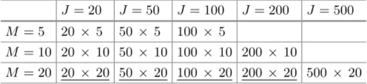
For the PFSP, the most often used benchmark set is developed by Taillard [7]. This benchmark set can be divided in 12 (J×M) sets with 10 instances each (See Table1). The instances are a selection of the hardest randomly generated instances. Here, instances for which simple metaheuristics do not often find the same solution or where the solution is far from a lower bound are considered to be hard.
Structured Instances
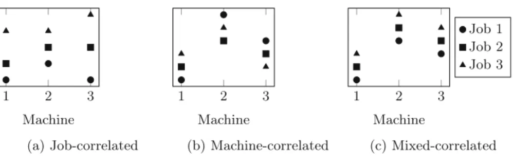
Aalvanger [1] introduced a new set of benchmarks for testing algorithms on structured instances. The benchmark set contains the three types of struc-tured instances as described by Watson [10]: Job-correlated (JC), Machine-correlated (MC) and Mixed-Machine-correlated (MXC) instances (see Fig.1). In job-correlated instances, processing times are dependent on the job and not on the machines. Therefore the processing times of operations in one job are related. In machine-correlated instances the structure goes the other way around. Here, processing times on one machine are related, while processing times within one job are unrelated. Mixed-correlated instances are equal to Machine-correlated instances, but here the relative ranks of processing times within each machine are job-dependent.
Fig. 1.Job processing time for three types of structured PFSP instances.
For each of the three correlation types, four (J × 20) sets are generated (See underlined in Table1). For each instance size, 1100 instances are generated, with varying values for correlation: α∈ {0.0,0.1· · ·1.0}. Forα= 0.0, instances reflect the way Taillard instances are generated, higher values introduce more correlation. Forα= 1.0, every task in a job/machine has the same processing time.
3.2 Comparing Results
To compare algorithms for PFSP, the Relative Percentage Deviation (RPD) is often used. The RPD describes the relative distance to the best known upper
Table 1.Sizes of the Taillard PFSP instances, for underlined sizes structured instances are available. J= 20 J= 50 J= 100 J= 200 J= 500 M = 5 20×5 50 ×5 100×5 M = 10 20×10 50 ×10 100×10 200 ×10 M = 20 20×20 50 ×20 100×20 200 ×20 500× 20
bound (UB) of an instance and the result of the algorithm RES. The RPD is calculated by
RP D(RES) = 100·(RES−UB)
UB . (6)
RPD values are best used when the upper bound is very close to the opti-mal solution. An RPD value of 0.0 then means that the optimal solution has been found. Over a set of runs, the average or median RPD is often reported (ARPD/MRPD). In our results, we also report the average over the MRPDs of multiple instances (AMRPD).
We use the Mann-Whitney-U test to check for a significant difference between two algorithms. Unless reported otherwise, we use sample sizes of 20 per instance to find MRPD values. AMRPD values are found over 10 instances with the same size. For significance tests we use a significance level ofp <0.05.
4
Heuristics for the PFSP
4.1 Constructive HeuristicsFor the TFT criterion, Liu and Reeves have introduced the LR(x) heuristic [6], which can generate up to J schedules, depending on the parameter x. LR(x) builds a schedule from the front to the back, using the following three steps: 1. Sort all jobs according to the index function.
2. Createxpartial schedules with the top-x jobs scheduled first. Extend the par-tial schedules by iteratively adding the best job according to the re-evaluated index function.
3. Select the best schedule generated in step 2).
The index function for adding jobi after the last job k in the partial schedule consists of two components:
1. A weighted total machine idle time, penalizing the time the machines wait between job k and job i. Idle time on the first machines is punished more than idle time on the last machines.
2. Theartificial total flow time, is the sum of the completion time of jobiplus the completion time of an artificial job representing the unscheduled jobs.
Fig. 2. Seeding with the LR heuristics: amount of seeds vs. solution quality after 50,000,000 fitness evaluations.
4.2 Constructive Heuristics Seeding: Results
For the LR heuristic we have tested the effect of seeding solutions in the initial populations of permutation GOMEA. Figure2 shows that for most instances -especially the larger ones - more seeds result in better solutions. This holds for both structured and unstructured instances. An interesting observation is the effect of single-solution seeding. Here, the dominant new solution can misguide optimal mixing, leading to worse solutions.
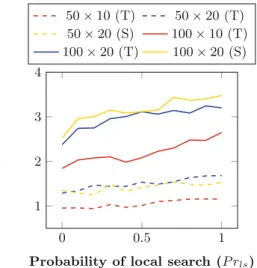
Fig. 3. Hybrid GOMEA performance with respect to the probability of local search for Taillard (T) and structured (S) instances (α= 0.3)
4.3 Improvement Heuristics
For the PFSP with the TFT criterion, various improvement heuristics exist. Each of these improvement heuristics are based on two fundamental permu-tation neighborhoods: job insertion and job swap. The swap heuristic takes two jobs and swaps them in a permutation. The insertion heuristic takes one job and puts it in another place in the permutation. Both heuristics have a neighbor-space that is quadratic in the amount of jobs and takeO(J ·M) time to compute the fitness of a neighbor. In permutation GOMEA an improvement heuristic is most effectively applied when a solution has changed in the GOM phase. For permutation GOMEA solving the PFSP with the TFT criterion, the swap heuristic was shown to have the most potential, especially on instances with a few machines (for more details see [1]). Figure3 shows for structured (mixed-correlation) and unstructured instances how permutation GOMEA per-forms when this improvement heuristic is applied with some probability P rls. Clearly, the use of the neighborhood search does not improve the effectiveness of permutation GOMEA within the given computational time budget. Apparently the extensive search already executed by the Gene-pool Optimal Mixing process does not benefit anymore from the classical swap neighborhood exploration.
5
Permutation GOMEA vs. VNS4 Iterated Local Search
The previous section showed that permutation GOMEA can best be enhanced by seeding the initial population with solutions constructed with the LR heuristic. Adding local search to improve each solution after the gene-pool mixing process does not result in consistent improvements on all instances, and is thereforeTable 2.Quality of pGOMEA and VNS4 on Taillard instances.
not applied in this section. To see how well permutation GOMEA performs in comparison with a well tested Iterated Local Search heuristic for the PFSP, we compare it with VNS4, a Variable Neighborhood Search algorithm which uses an optimal form of combining the insertion heuristic and swap heuristic in order to solve the PFSP with the TFT criterion [4]. VNS4 was the most successful algorithm in a study of six different ways to combine the two most used neighborhoods in the literature used for the permutation flowshop scheduling problem with total flowtime criterion, namely job interchange and job insertion. VNS4 turned out to be the most effective of the six variable neighborhood search algorithms. VNS4 was also compared to a state-of-the-art evolutionary approach which it outperformed on most of the benchmark instances.
VNS4 is started from a solution generated by the LR constructive heuristic. First, VNS4 fully explores the job interchange neighborhood until no further improvement is possible. Then, a single iteration of the job insertion neigh-borhood search is executed. If this iteration improves the current solution, the algorithm resumes the interchange neighborhood search. When a local optimum common to both neighborhoods has been reached within the computational time limit, VNS4 executes a random walk to escape from the region of attraction of this local optimum. The random walk consists ofkrandom job insertion moves. Iterated Local Search is sensitive to the length of the perturbation size. Exper-imental results show that VNS4’s performance degrades when the perturbation
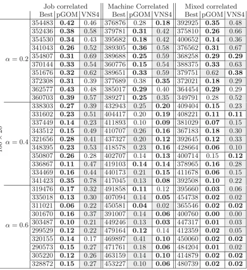
Table 3.Quality of pGOMEA and VNS4 on structured instances.
size is less than 14 or greater than 18 random job insertion moves [4]. The results with 14≤k≤18 produce very similar results, butk= 14 has the lowest RPD median, so this value is shown here in the Tables with experimental results.
Table2shows the MRPD values on Taillard problem instances for VNS4 and permutation GOMEA when both algorithms are run for 400·J·Mmilliseconds. This stopping criterion is the same as used in recent works of [5,8,11] which were all included in the comparison in [4].
The best solution in the Table is marked bold and if the other solution performs significantly worse, its cell is marked grey. The results show that in most cases permutation GOMEA outperforms VNS4 significantly, in a number of cases there is no statistically significant difference, and in only a few instances VNS4 outperforms permutation GOMEA.
Secondly, we have tested permutation GOMEA and VNS4 on multiple struc-tured instances with size 100×20. For these problems we have run the algorithms for 400·(1−α)·J·Mseconds, as structure makes the problems easier. Table3 shows the results for three types of structured instances and threeαvalues.
The results show for job-correlated instances that permutation GOMEA always outperforms the VNS4 algorithm. The type of structure apparently suits permutation GOMEA best, while VNS4 cannot benefit from an easier fitness landscape. The machine-correlated instances with a high amount of structure (α ≥ 0.4) are however easier for VNS4. When machine and job correlation are mixed, the PFSP is best solved using permutation GOMEA. Permutation GOMEA finds solutions with MRPD values lower than 0.5, showing that struc-tured instances are easier than the standard Taillard instances.
An interesting question is why permutation GOMEA does not outperform VNS4 for the machine-correlated instances with a high amount of structure? Apparently, permutation GOMEA does not fully capture the structure in the machine-related instances. The most likely explanation is that this structure is not represented well enough in the distance measure used to build the linkage tree. Further research into the relation between the structure in specific problem instances and the type of structure searched for by GOMEA using different distance measures is needed to answer this question.
6
Conclusions
Previous work has shown how the Gene-pool Optimal Mixing Evolutionary Algo-rithm can be applied to permutation problems like the PFSP by representing solutions with the random-key encoding. Each generation GOMEA builds a link-age tree in order to capture structure in the set of solutions. This linklink-age tree can also be looked upon as an adaptive neighborhood learned by GOMEA to explore new solutions. In this paper we have investigated how the use of constructive heuristics and neighborhood search might improve on the Black-Box approach of permutation GOMEA. Results showed that adding neighborhood search does not consistently improve the performance. However, seeding the initial popula-tion of GOMEA by solupopula-tions generated by the constructive LR heuristic was shown to be an effective technique. We have experimentally compared permu-tation GOMEA - seeded with the constructive heuristic LR - with the highly successful VNS4 algorithm for unstructured and structured Permutation Flow-shop Scheduling problems. VNS4 is an Iterated Local Search algorithm using a variable neighborhood that combines the job insertion neighborhood with the job swap neighborhood.
For the unstructured Taillard instances, GOMEA almost always outper-forms VNS4. Also for the job correlated structured instances and for the mixed job/machine correlated instances GOMEA outperforms VNS4. Only for machine correlated structured instances with a high amount of structure (α≥0.4), VNS4 outperforms permutation GOMEA.
As a general conclusion, this paper has shown that the use of a multi-solution constructive heuristic to seed the initial population of permutation GOMEA
leads to an effective model-based evolutionary algorithm. It has also been shown that adding neighborhood search algorithms does not always result in more efficient results given a fixed computational time budget.
References
1. Aalvanger, G.: Incorporating domain knowledge in permutation gene-pool optimal mixing evolutionary algorithms. Master’s thesis. Utrecht University, The Nether-lands (2017).https://dspace.library.uu.nl/handle/1874/353005
2. Bosman, P.A., Luong, N.H., Thierens, D.: Expanding from discrete Cartesian to permutation gene-pool optimal mixing evolutionary algorithms. In: Proceedings of the Genetic and Evolutionary Computation Conference, pp. 637–644. ACM (2016) 3. Ceberio, J., Irurozki, E., Mendiburu, A., Lozano, J.A.: Extending distance-based ranking models in estimation of distribution algorithms. In: 2014 IEEE Congress on Evolutionary Computation, CEC, pp. 2459–2466, July 2014
4. Costa, W.E., Goldbarg, M.C., Goldbarg, E.G.: New VNS heuristic for total flow-time flowshop scheduling problem. Expert Syst. Appl.39(9), 8149–8161 (2012) 5. Jarboui, B., Eddaly, M., Siarry, P.: An estimation of distribution algorithm for
min-imizing the total flowtime in permutation flowshop scheduling problems. Comput. Oper. Res.36, 2638–2646 (2009)
6. Liu, J., Reeves, C.R.: Constructive and composite heuristic solutions to the p||Ci scheduling problem. EJOR132(2), 439–452 (2001)
7. Taillard, E.: Benchmarks for basic scheduling problems. Eur. J. Oper. Res.64(2), 278–285 (1993)
8. Tasgetiren, M.F., Pan, Q.-K., Suganthan, P.N., Chen, A.H.-L.: A discrete artificial bee colony algorithm for the permutation flow shop scheduling problem with total flowtime criterion. In: Proceedings of the IEEE World Congress on Computational Intelligence, WCCI-2010, pp. 137–144. IEEE (2010)
9. Thierens, D., Bosman, P.A.: Optimal mixing evolutionary algorithms. In: Proceed-ings of the Genetic and Evolutionary Computation Conference, pp. 617–624 (2011) 10. Watson, J.-P., Barbulescu, L., Whitley, L.D., Howe, A.E.: Contrasting structured and random permutation flow-shop scheduling problems. INFORMS J. Comput.
14(2), 98–123 (2002)
11. Xu, X., Xu, Z., Gu, X.: An asynchronous genetic local search algorithm for the per-mutation flowshop scheduling problem with total flowtime minimization. Expert Syst. Appl.38, 7970–7979 (2011)