SPADE: An Efficient Algorithm for Mining Frequent Sequences

SPADE: An Efficient Algorithm for Mining

Frequent Sequences

MOHAMMED J. ZAKI [email protected]

Computer Science Department, Rensselaer Polytechnic Institute, Troy NY 12180-3590

Editor: Douglas Fisher

Abstract. In this paper we present SPADE, a new algorithm for fast discovery of Sequential Patterns. The existing solutions to this problem make repeated database scans, and use complex hash structures which have poor locality. SPADE utilizes combinatorial properties to decompose the original problem into smaller sub-problems, that can be independently solved in main-memory using efficient lattice search techniques, and using simple join operations. All sequences are discovered in only three database scans. Experiments show that SPADE outperforms the best previous algorithm by a factor of two, and by an order of magnitude with some pre-processed data. It also has linear scalability with respect to the number of input-sequences, and a number of other database parameters. Finally, we discuss how the results of sequence mining can be applied in a real application domain.

Keywords: sequence mining, sequential patterns, frequent patterns, data mining, knowledge discovery

1. Introduction

The sequence mining task is to discover a set of attributes, shared across time among a large number of objects in a given database. For example, consider the sales database of a bookstore, where the objects represent customers and the attributes represent authors or books. Let’s say that the database records the books bought by each customer over a period of time. The discovered patterns are the sequences of books most frequently bought by the customers. An example could be that, “70% of the people who buy Jane Austen’s Pride and Prejudice also buy Emma within a month.” Stores can use these patterns for promotions, shelf placement, etc. Consider another example of a web access database at a popular site, where an object is a web user and an attribute is a web page. The discovered patterns are the sequences of most frequently accessed pages at that site. This kind of information can be used to restructure the web-site, or to dynamically insert relevant links in web pages based on user access patterns. Other domains where sequence mining has been applied include identifying plan failures (Zaki, Lesh, & Ogihara, 1998), finding network alarm patterns (Hatonen et al., 1996), and so on.

The task of discovering all frequent sequences in large databases is quite challenging. The search space is extremely large. For example, with m attributes there are O(mk₎

potentially frequent sequences of length k. With millions of objects in the database the problem of I/O minimization becomes paramount. However, most current algorithms are iterative in nature, requiring as many full database scans as the longest frequent sequence;

of objects in which it occurs, along with the time-stamps. We show that all frequent sequences can be enumerated via simple temporal joins (or intersections) on id-lists. 2. We use a lattice-theoretic approach to decompose the original search space (lattice) into

smaller pieces (sub-lattices) which can be processed independently in main-memory. Our approach usually requires three database scans, or only a single scan with some pre-processed information, thus minimizing the I/O costs.

3. We decouple the problem decomposition from the pattern search. We propose two different search strategies for enumerating the frequent sequences within each sub-lattice: breadth-first and depth-first search.

SPADE not only minimizes I/O costs by reducing database scans, but also minimizes computational costs by using efficient search schemes. The vertical id-list based approach is also insensitive to data-skew. An extensive set of experiments shows that SPADE out-performs previous approaches by a factor of two, and by an order of magnitude if we have some additional off-line information. Furthermore, SPADE scales linearly in the database size, and a number of other database parameters.

We also briefly discuss how sequence mining can be applied in practice. We show that in complicated real-world applications, sequence mining can produce an overwhelming number of frequent patterns. We discuss how one can identify the most interesting patterns using pruning strategies in a post-processing step.

The rest of the paper is organized as follows: In Section 2 we describe the sequence discovery problem and look at related work in Section 3. In Section 4 we develop our lattice-based approach for problem decomposition, and for pattern search. Section 5 describes our new algorithm. An experimental study is presented in Section 6. Section 7 discusses how the sequence mining can be used in a realistic domain. Finally, we conclude in Section 8.

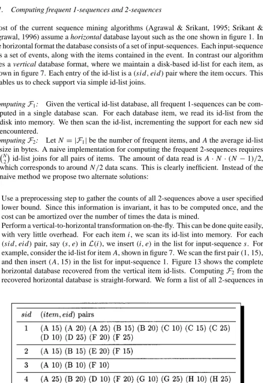
2. Problem statement

The problem of mining sequential patterns can be stated as follows: LetI = {i1,i2, . . . ,im} be a set of m distinct items comprising the alphabet. An event is a non-empty unordered collection of items (without loss of generality, we assume that items of an event are sorted in lexicographic order). A sequence is an ordered list of events. An event is denoted as (i1i2. . .ik), where ij is an item. A sequenceαis denoted as(α1 → α2 → · · · → αq),

whereαi is an event. A sequence with k items (k = P

j|αj|) is called a k-sequence. For

example,(B→ AC)is a 3-sequence.

For a sequenceα, if the eventαi occurs beforeαj, we denote it as αi < αj. We say

αis a subsequence of another sequenceβ, denoted asα¹ β, if there exists a one-to-one order-preserving function f that maps events inαto events inβ, that is, 1)αi ⊆ f(αi), and

2) ifαi < αjthen f(αi) < f(αj). For example the sequence(B→ AC)is a subsequence

of (A B → E → AC D), since B ⊆ A B and AC ⊆ AC D, and the order of events is preserved. On the other hand the sequence(A B → E)is not a subsequence of(A B E), and vice versa.

The databaseDfor sequence mining consists of a collection of input-sequences. Each input-sequence in the database has an unique identifier called sid, and each event in a given input-sequence also has a unique identifier called eid. We assume that no sequence has more than one event with the same time-stamp, so that we can use the time-stamp as the event identifier.

An input-sequence C is said to contain another sequenceα, ifα ¹ C, i.e., if αis a subsequence of the input-sequenceC. The support or frequency of a sequence, denoted σ (α,D), is the the total number of input-sequences in the databaseDthat containα. Given a user-specified threshold called the minimum support (denoted min sup), we say that a sequence is frequent if it occurs more than min sup times. The set of frequent k-sequences is denoted asFk. A frequent sequence is maximal if it is not a subsequence of any other

frequent sequence.

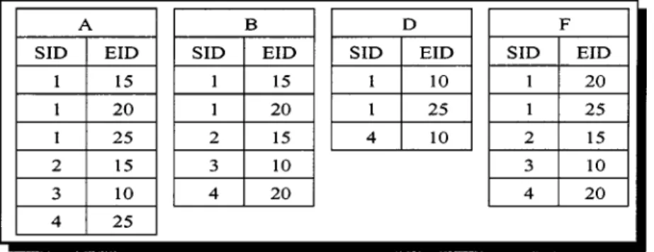
Given a databaseDof input-sequences and min sup, the problem of mining sequential patterns is to find all frequent sequences in the database. For example, consider the input database shown in figure 1 (used as a running example throughout this paper). The database

all the frequent sequences with a minimum support of 50% (i.e., a sequence must occur in at least 2 input-sequences). In this example we have a two maximal frequent sequences,

A B F and D→B F → A.

Some comments are in order to see the generality of our problem formulation: 1) We discover sequences of subsets of items, and not just single item sequences. For example, the set B F in(D→B F → A). 2) We discover sequences with arbitrary gaps among events, and not just the consecutive subsequences. For example, the sequence(D→ B F → A) is a subsequence of input-sequence 1, even though there is an intervening event between D and B F . The sequence symbol→simply denotes a happens-after relationship. 3) Our formulation is general enough to encompass almost any categorical sequential domain. For example, if the input-sequences are DNA strings, then an event consists of a single item (one of A,C,G,T ). If input-sequences represent text documents, then each word (along with any other attributes of that word, e.g., noun, position, etc.) would comprise an event. Even continuous domains can be represented after a suitable discretization step.

2.1. Sequence rules

Once the frequent sequences are known, they can be used to obtain rules that describe the relationship between different sequence items. For example, the sequence(B F)occurs in four input-sequences, while(A B F)in three input-sequences. We can therefore say that if B F occurs together, then there is a 75% chance that A also occurs. In other words we say that the rule(B F) ⇒ (A B F)has a 75% confidence. Another example of a rule is that(D → B F)⇒(D → B F → A). It has 100% confidence. Given a user-specified minimum confidence (min conf), we can generate all rules that meet the condition by means of the simple algorithm shown in figure 2. Since the rule generation step is relatively straightforward, in the rest of the paper we will mainly concentrate on the frequent sequence discovery phase. We do return to the problem of generating useful rules, in Section 7, within a planning domain.

3. Related work

The problem of mining sequential patterns was introduced in Agrawal and Srikant (1995). They also presented three algorithms for solving this problem. The AprioriAll algorithm

was shown to perform better than the other two approaches. In subsequent work (Srikant & Agrawal, 1996), the same authors proposed the GSP algorithm that outperformed AprioriAll by up to 20 times. They also introduced maximum gap, minimum gap, and sliding window constraints on the discovered sequences.

Independently, Mannila, Toivonen, and Verkamo (1995) proposed mining for frequent episodes, which are essentially frequent sequences in a single long input-sequence (typically, with single items events, though they can handle set events). However our formulation is geared towards finding frequent sequences across many different input-sequences. They further extended their framework in Mannila and Toivonen (1996) to discover generalized episodes, which allows one to express arbitrary unary conditions on individual sequence events, or binary conditions on event pairs. The MEDD and MSDD algorithms (Oates et al., 1997) discover patterns in multiple event sequences; they explore the rule space directly instead of the sequence space.

Sequence discovery can essentially be thought of as association discovery (Agrawal et al., 1996; Savasere, Omiecinski, & Navathe, 1995) over a temporal database. While association rules discover only intra-event patterns (called itemsets), we now also have to discover inter-event patterns (sequences). The set of all frequent sequences is a superset of the set of frequent itemsets. Due to this similarity sequence mining algorithms like AprioriAll, GSP, etc., utilize some of the ideas initially proposed for the discovery of association rules. Our new algorithm is based on the fast association mining techniques we presented in Zaki et al. (1997). Nevertheless, the sequence search space is much more complex and challenging than the itemset space, and thus warrants specific algorithms. A preliminary version of this paper appeared in Zaki (1998).

3.1. The GSP algorithm

Below we describe the GSP algorithm (Srikant & Agrawal, 1996) in some more detail, since we use it as a base against which we compare SPADE, and it is one of the best previous algorithms.

GSP makes multiple passes over the database. In the first pass, all single items (1-sequences) are counted. From the frequent items a set of candidate 2-sequences are formed. Another pass is made to gather their support. The frequent 2-sequences are used to generate the candidate 3-sequences, and this process is repeated until no more frequent sequences are found. There are two main steps in the algorithm.

1. Candidate Generation: Given the set of frequent(k−1)-sequencesFk−1, the candidates for the next pass are generated by joiningFk−1with itself. A pruning phase eliminates any sequence at least one of whose subsequences is not frequent. For fast counting, the candidate sequences are stored in a hash-tree.

2. Support Counting: To find all candidates contained in a input-sequenceE, conceptually all k-subsequences ofE are generated. For each such subsequence a search is made in the hash-tree. If a candidate in the hash-tree matches the subsequence, its count is incremented.

The GSP algorithm is shown in figure 3. For more details on the specific mechanisms for constructing and searching hash-trees, please refer to Srikant and Agrawal (1996).

4. Sequence enumeration: Lattice-based approach

Before embarking on the algorithm description, we will briefly review some terminology from lattice theory (see Davey and Priestley (1990) for a good introduction).

Definition 1. Let P be a set. A partial order on P is a binary relation≤, such that for all X,Y,Z ∈ P, the relation is:

1) Reflexive: X ≤ X .

2) Anti-Symmetric: X ≤Y and Y ≤ X , implies X =Y . 3) Transitive: X ≤Y and Y ≤Z , implies X ≤ Z .

The set P with the relation≤is called an ordered set.

Definition 2. Let P be an ordered set, and let S ⊆ P. An element X ∈ P is an upper bound (lower bound ) of S if s ≤ X (s≥ X ) for all s ∈ S. The minimum (or least) upper bound, called the join, of S is denoted as∨S, and the maximum (or greatest) lower bound, called the meet, of S is denoted as∧S. The greatest element of P, denoted>, is called the top element, and the least element of P, denoted⊥, is called the bottom element.

Definition 3. Let L be an ordered set. L is called a join (meet) semilattice if X∨Y (X∧Y ) exists for all X,Y ∈ L, i.e., the minimum upper bound (maximum lower bound) exists. L is called a lattice if it is a join and meet semilattice. A ordered set M⊂L is a sublattice of L if X,Y ∈M implies X ∨Y ∈M and X∧Y ∈M.

Definition 4. Let L be a lattice, and let X,Z,Y ∈L. We say X is covered by Y , if X <Y and X ≤Z <Y , implies Z =X , i.e., if there is no element Z of L with X <Z <Y . Let

⊥be the bottom element of lattice L. Then X ∈ L is called an atom if X covers⊥. The set of atoms of L is denoted byA(L).

Definition 5. Let L be an ordered set. L is called a hyper-lattice if X∨Y (X∧Y ), instead of representing a unique minimum upper bound (maximum lower bound), represents a set of minimal upper bounds (maximal lower bounds).

Note that in a regular lattice the join and meet refers to the unique minimum upper bound and maximum lower bound. In a hyper-lattice the join and meet need not produce a unique element; instead the result can be a set of minimal upper bounds and maximal lower bounds. In the rest of this paper we will usually refer to the sequence hyper-lattice as a lattice (unless we wish to stress the difference), since the sequence context is understood.

Lemma 1. LetS be the set of all sequences on the items inI. Then the subsequence relation¹, defines a hyper-lattice onS.

Theorem 1. Given a setI of items, the ordered setS of all possible sequences on the items, is a hyper-lattice in which the join of a set of sequences Ai∈Sis the set of minimal

common supersequences, and the meet of a set of sequences is the set of maximal common subsequences. More formally,

_

{Ai} = {α| Ai ¹αand Ai ¹βwithβ¹α⇒β=α} ^

{Ai} = {α|α¹ Ai andβ ¹ Aiwithα¹β ⇒β=α}

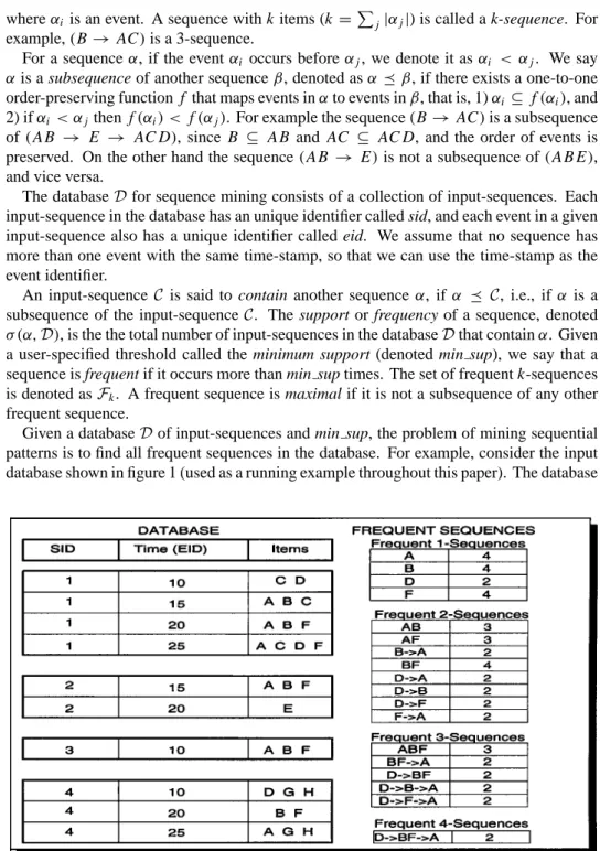
From our example database (figure 1), the set of frequent items is given as F1 = {A,B,D,F}. Figure 4 shows the sequence latticeS spanned by the subsequence rela-tion on these four frequent items. These are also the atoms of the sequence lattice, since they cover the bottom element{}. To see why the set of all sequences forms a hyper-lattice, consider the join of A and B; A∨ B = {(A → B), (A B), (B → A)}. As we can see the join produces three minimal upper bounds (i.e., minimal common super-sequences). Similarly, the meet of two (or more) sequences can produce a set of maximal lower bounds. For example, (B → A B)∧(A B → A) = {(A B), (B → A)}, both of which are the maximal common sub-sequences.

The bottom element of the sequence lattice is⊥ = {}, but the top element is undefined, since in the abstract the sequence lattice is infinite. Thus figure 4 shows only some parts of the lattice, namely, the complete set of 2-sequences, the 3-sequences that can be generated from A→ A and A B, and the possible 4-sequences that can be generated from A → A → A. The recursive combinatorial structure of the subsequence lattice should be apparent. For example consider the set of sequences generated from the item A, and the sequence A→ A. The two sets are identical except for the extra A→prefix in the latter set.

Lemma 2. Let n denote the number of frequent items. Then the total number of sequences of length at most k is O(nk).

Proof. We will count the number of ways in which a k sequence can be constructed, and then assign items for each arrangement. The number of ways a k-sequence can be constructed is given by the number of ways we can obtain k as a sum of integers. For

Figure 4. Sequence lattice spanned by subsequence relation.

Figure 5. Number of ways to obtain a 4-sequence.

example, figure 5 shows the number of ways we can obtain 4 as a sum of integers. The integers in the sum are interpreted to be the sizes of the events comprising a k length sequence. We now assign items to each such event. For an event of length i , we have¡n_i¢ item assignments. Multiplying the choices for each case, and adding all the cases we obtain the total number of k-sequences, given asPk_i

1=1 ¡_n i1 ¢ Pk₋i1 i2=1 ¡_n i2 ¢ · · ·Pk−i1−···−ik−1 ik=1 ¡_n ik ¢ . It is difficult to derive a closed-form expression for the exact number of k-sequences from the formula above, but a closed-form expression for an upper-bound on the number of k-sequences can be obtained as follows. For each of the k positions we have the choice of

Figure 6. Lattice induced by maximal frequent sequences A B F and D→B F→A.

n items, and between items we have two choices: to put a→or not. Thus, the total number of k-sequences is bounded above by the expression 2k−1_nk_{. Then, the total number of}

se-quences of length at most k is given asPk_i=12i−1_ni _≤2k−1Pk i=1n

i_≈2k−1_nk_=O(nk_{), for}

a constant k. ¤

As mentioned above, in the abstract case the lattice of sequences is infinite. Fortunately in all practical cases it is bounded. The number of sequence elements (events) is bounded above by the maximum number of events per input-sequence (say C). Since the size of an event is bounded above by the maximum event size (say T ), a sequence can have at most C·T items, and hence the subsequence lattice is bounded above by C·T . In our example database, C =4 and T =4, so that the largest possible sequence can have 16 items.

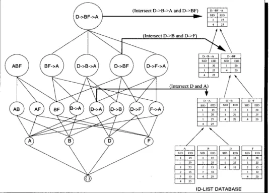
In all practical cases not only is the lattice bounded, but the set of frequent sequences is also very sparse (depending on the min sup value). For example, consider figure 6 which shows the sequence lattice induced by the maximal frequent sequences A B F and D → B F → A, in our example. The set of atoms A is given by the frequent items

{A,B,D,F}. It is obvious that the set of all frequent sequences forms a meet-semilattice, because it is closed under the meet operation, i.e., if X and Y are frequent sequences, then the meet X ∧Y (a maximal common subsequence) is also frequent. However, it is not a join-semilattice, since it is not closed under joins, i.e., X and Y being frequent, doesn’t imply that X∨Y (a minimal common supersequence) is frequent. The closure under meet leads to the well known observation on sequence frequency:

Lemma 3. All subsequences of a frequent sequence are frequent.

The above lemma leads very naturally to a bottom-up search procedure for enumerating frequent sequences, which has been leveraged in many sequence mining algorithms (Srikant

Figure 7. Id-lists for the atoms.

& Agrawal, 1996; Mannila, Toivonen, & Verkamo, 1995; Oates et al., 1997). In essence what the lemma says is that we need to focus only on those sequences whose subsequences are frequent. This leads to a very powerful pruning strategy, where we eliminate all se-quences, at least one of whose subsequences is infrequent. However, the lattice formulation makes it apparent that we need not restrict ourselves to a purely bottom-up search. We can employ different search procedures, which we will discuss below.

4.1. Support counting

Let’s associate with each atom X in the sequence lattice its id-list, denotedL(X), which is a list of all input-sequence (sid) and event identifier (eid) pairs containing the atom. Figure 7 shows the id-lists for the atoms in our example database. For example consider the atom D. In our original database in figure 1, we see that D occurs in the following input-sequence and event identifier pairs{(1,10), (1,25), (4,10)}. This forms the id-list for item D. Lemma 4. For any X∈S, let J= {Y∈A(S)|Y¹X}. Then X= ∨Y_∈JY , andσ(X)= | ∩Y∈J L(Y)|, where ∩ denotes a temporal join of the id-lists, and |L(Z)|, called the

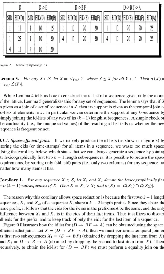
cardinality ofL(Z), denotes the number of distinct sid values in the id-list for a sequence Z . The above lemma states that any sequence inScan be obtained as a temporal join of some atoms of the lattice, and the support of the sequence can be obtained by joining the id-list of the atoms. Let’s say we wish to compute the support of sequence(D → B F → A). Here the set J = {D,B,F,A}. We can perform temporal joins one atom at a time to obtain the final id-list, as shown in figure 8. We start with the id-list for atom D and join it with that of B. Since the symbol→represents a temporal relationship, we find all occurrences of B after a D in an input-sequence, and store the corresponding time-stamps or eids, to obtainL(D→ B). We next join the id-list of(D→ B)with that of atom F , but this time the relationship between B and F is a non-temporal one, which we call an equality join, since they must occur at the same time. We thus find all occurrences of B and F with the same eid and store them in the id-list for(D→ B F). Finally, a temporal join withL(A) completes the process.

Figure 8. Naive temporal joins.

Lemma 5. For any X∈S, let X= ∨Y_∈J Y , where Y¹X for all Y∈J . Thenσ(X)= |∩Y∈JL(Y)|.

While Lemma 4 tells us how to construct the id-list of a sequence given only the atoms of the lattice, Lemma 5 generalizes this for any set of sequences. The lemma says that if X is given as a join of a set of sequences in J , then its support is given as the temporal join of id-lists of elements in J . In particular we can determine the support of any k-sequence by simply joining the id-lists of any two of its(k−1)length subsequences. A simple check on the cardinality (i.e., the unique sid values) of the resulting id-list tells us whether the new sequence is frequent or not.

4.1.1. Space-efficient joins. If we naively produce the id-lists (as shown in figure 8) by storing the eids (or time-stamps) for all items in a sequence, we waste too much space. Using the corollary below, which states that we can always generate a sequence by joining its lexicographically first two k−1 length subsequences, it is possible to reduce the space requirements, by storing only (sid, eid) pairs (i.e., only two columns) for any sequence, no matter how many items it has.

Corollary 1. For any sequence X ∈S, let X1and X2 denote the lexicographically first

two(k−1)-subsequences of X . Then X =X1∨X2andσ(X)= |L(X1)∩L(X2)|. The reason why this corollary allows space reduction is because the first two k−1 length sequences, X1and X2, of a sequence X , share a k−2 length prefix. Since they share the same prefix, it follows that the eids for the items in the prefix must be the same, and the only difference between X1and X2is in the eids of their last items. Thus it suffices to discard all eids for the prefix, and to keep track of only the eids for the last item of a sequence.

Figure 9 illustrates how the idlist for(D→B F → A)can be obtained using the space-efficient idlist joins. Let X =(D→ B F → A), then we must perform a temporal join on its first two subsequences X1 =(D→ B F)(obtained by dropping the last item from X ), and X2 = D → B → A (obtained by dropping the second to last item from X ). Then, recursively, to obtain the id-list for(D → B F)we must perform a equality join on the

Figure 9. Computing support via space-efficient temporal id-list joins.

id-list of(D→ B)and(D→ F). For(D→ B → A)we must perform a temporal join onL(D→ B)andL(D→ A). Finally, the 2-sequences are obtained by joining the atoms directly. Figure 9 shows the complete process, starting with the initial vertical database of the id-list for each atom. As we can see, at each point only (sid,eid) pairs are stored in the id-lists (i.e., only the eid for the last item of a sequence are stored). The exact details of the temporal joins are provided in Section 5.3, when we discuss the implementation of SPADE. Lemma 6. Let X and Y be two sequences , with X ¹Y . Then|L(X)| ≥ |L(Y)|.

This lemma says that if the sequence X is a subsequence of Y , then the cardinality of the id-list of Y (i.e., its support) must be equal to or less than the cardinality of the id-list of X . A practical and important consequence of this lemma is that the cardinalities of intermediate id-lists shrink as we move up the lattice. This results in very fast joins and support counting.

4.2. Lattice decomposition: Prefix-based classes

If we had enough main-memory, we could enumerate all the frequent sequences by travers-ing the lattice, and performtravers-ing temporal joins to obtain sequence supports. In practice,

Figure 10. a) Equivalence classes ofSinduced byθ1, b) classes of [D]θ1induced byθ2.

however, we only have a limited amount of main-memory, and all the intermediate id-lists will not fit in memory. This brings up a natural question: can we decompose the original lat-tice into smaller pieces such that each piece can be solved independently in main-memory. We address this question below.

Define a function p:(S,N)→S whereSis the set of sequences, N is the set of non-negative integers, and p(X,k)= X [1 : k]. In other words, p(X,k)returns the k length prefix of X . Define an equivalence relationθkon the latticeSas follows: ∀X,Y ∈S, we

say that X is related to Y underθk, denoted as X ≡θk Y if and only if p(X,k)= p(Y,k).

That is, two sequences are in the same class if they share a common k length prefix. Figure 10 shows the partition induced by the equivalence relationθ1 onS, where we collapse all sequences with a common item prefix into an equivalence class. The resulting set of equivalence classes is{[ A],[B],[D],[F ]}. We call these first level classes as the parent classes. At the bottom of the figure, it also shows the links among the four classes. These links carry pruning information. In other words if we want to prune a sequence (if it has at least one infrequent subsequence) then we may need some cross-class information. We will have more to say about this later in Section 5.4.

Lemma 7. Each equivalence class [X ]_θk induced by the equivalence relationθk is a

sub-(hyper)lattice ofS.

Proof. Let U and V be any two elements in the class [X ], i.e., U,V share the common prefix X . Thus X ¹Z for all Z ∈U∨V , i.e., since U and V share a common prefix, then so must any minimal common super-sequence. This implies that Z∈[X ] for all Z∈U∨V . On the other hand, since U and V share a common prefix, then so must any maximal

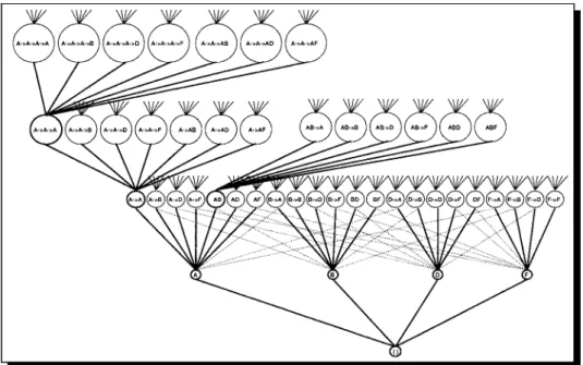
scenario, we apply recursive class decomposition. Let’s assume that [D] is too large to fit in main-memory. Since [D] is itself a lattice, it can be decomposed using the relationθ2. Figure 10 shows the classes induced by applyingθ2on [D] (after applyingθ1onS). Each of the resulting six parent classes, [ A], [B], [D→ A], [D→ B], [D →F ], and [F ], can be processed independently to generate frequent sequences from each class. Thus depending on the amount of main-memory available, we can recursively partition large classes into smaller ones, until each class is small enough to be solved independently in main-memory.

4.3. Search for frequent sequences

In this section we discuss efficient search strategies for enumerating the frequent sequences within each parent class. We will discuss two main strategies: breadth-first and depth-first search. Both these methods are based on a recursive decomposition of each parent class into smaller classes induced by the equivalence relationθk. Figure 11 shows the decomposition

of [D]_θ1into smaller and smaller classes, and the resulting lattice of equivalence classes.

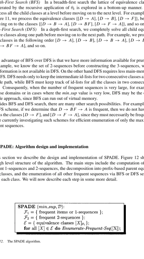
Breadth-First Search (BFS) In a breadth-first search the lattice of equivalence classes generated by the recursive application ofθk is explored in a bottom-up manner. We

process all the child classes at a level before moving on to the next level. For example, in figure 11, we process the equivalence classes{[D→ A],[D→ B],[D→ F ]}, before moving on to the classes{[D→ B→ A],[D→ B F ],[D→ F→ A]}, and so on. Depth-First Search (DFS) In a depth-first search, we completely solve all child

equiva-lence classes along one path before moving on to the next path. For example, we process the classes in the following order [D → A], [D → B], [D→ B → A], [D → B F ], [D→ B F → A], and so on.

The advantage of BFS over DFS is that we have more information available for pruning. For example, we know the set of 2-sequences before constructing the 3-sequences, while this information is not available in DFS. On the other hand DFS requires less main-memory than BFS. DFS needs only to keep the intermediate id-lists for two consecutive classes along a single path, while BFS must keep track of id-lists for all the classes in two consecutive levels. Consequently, when the number of frequent sequences is very large, for example in dense domains or in cases where the min sup value is very low, DFS may be the only feasible approach, since BFS can run out of virtual memory.

Besides BFS and DFS search, there are many other search possibilities. For example, in the DFS scheme, if we determine that D→ B F → A is frequent, then we do not have to process the classes [D→ F ], and [D→ F→ A], since they must necessarily be frequent. We are currently investigating such schemes for efficient enumeration of only the maximal frequent sequences.

5. SPADE: Algorithm design and implementation

In this section we describe the design and implementation of SPADE. Figure 12 shows the high level structure of the algorithm. The main steps include the computation of the frequent 1-sequences and 2-sequences, the decomposition into prefix-based parent equiva-lence classes, and the enumeration of all other frequent sequences via BFS or DFS search within each class. We will now describe each step in some more detail.

ComputingF1: Given the vertical id-list database, all frequent 1-sequences can be com-puted in a single database scan. For each database item, we read its id-list from the disk into memory. We then scan the id-list, incrementing the support for each new sid encountered.

ComputingF2: Let N = |F1|be the number of frequent items, and A the average id-list size in bytes. A naive implementation for computing the frequent 2-sequences requires

¡N 2 ¢

id-list joins for all pairs of items. The amount of data read is A·N ·(N−1)/2, which corresponds to around N/2 data scans. This is clearly inefficient. Instead of the naive method we propose two alternate solutions:

1. Use a preprocessing step to gather the counts of all 2-sequences above a user specified lower bound. Since this information is invariant, it has to be computed once, and the cost can be amortized over the number of times the data is mined.

2. Perform a vertical-to-horizontal transformation on-the-fly. This can be done quite easily, with very little overhead. For each item i , we scan its id-list into memory. For each (si d,ei d)pair, say(s,e)inL(i), we insert(i,e)in the list for input-sequence s. For example, consider the id-list for item A, shown in figure 7. We scan the first pair(1,15), and then insert(A,15)in the list for input-sequence 1. Figure 13 shows the complete horizontal database recovered from the vertical item id-lists. ComputingF2from the recovered horizontal database is straight-forward. We form a list of all 2-sequences in

the list for each si d, and update counts in a 2-dimensional array indexed by the frequent items.

5.2. Enumerating frequent sequences of a class

Figure 14 shows the pseudo-code for the breadth-first and depth-first search. The input to the procedure is a set of atoms of a sub-lattice S, along with their id-lists. Frequent sequences are generated by joining the id-lists of all pairs of atoms (including a self-join) and checking the cardinality of the resulting list against min sup. Before joining the id-lists a pruning step can be inserted to ensure that all subsequences of the resulting sequence are frequent. If this is true, then we can go ahead with the id-list join, otherwise we can avoid the temporal join. Although SPADE supports pruning, we found that in practice, for the databases we looked at, it did not improve the running time. On the other hand, to successfully apply pruning, one has to store in memory all the frequent sequences found thus far. This imposes significant memory overheads, and thus in our experiments we disabled pruning. We discuss more details in Section 5.4.

The sequences found to be frequent at the current level form the atoms of classes for the next level. This recursive process is repeated until all frequent sequences have been enumerated. In terms of memory management it is easy to see that we need memory to store intermediate id-lists for at most two consecutive levels. The depth-first search requires memory for two classes on the two levels. The breadth-first search requires memory of all the classes on the two levels. Once all the frequent sequences for the next level have been generated, the sequences at the current level can be deleted.

Disk scans Before processing each parent equivalence class from the initial decompo-sition, all the relevant item id-lists for that class are scanned from disk into memory. The id-lists for the atoms (which are 2-sequences) of each initial class are constructed by joining

5.3. Temporal id-list join

We now describe how we perform the id-list joins for two sequences. Consider an equiva-lence class [B → A] with the atom set{B→ A B,B→ A D,B→ A→ A,B→ A→ D,B → A→ F}. If we let P stand for the prefix B→ A, then we can rewrite the class to get [P]= {P B,P D,P→ A,P→ D,P →F}. One can observe the class has two kinds of atoms: the event atoms{P B,P D}, and the sequence atoms{P→ A,P →D,P→ F}. We assume without loss of generality that the event atoms of a class always precede the sequence atoms. To extend the class it is sufficient to join the id-lists of all pairs of atoms. However, depending on the atom pairs being joined, there can be upto three possible result-ing frequent sequences (these are the three possible minimal common super-sequences): 1. Event atom with event atom: If we are joining P B with P D, then the only possible

outcome is new event atom P B D.

2. Event atom with sequence atom: If we are joining P B with P → A, then the only possible outcome is new sequence atom P B→ A.

3. Sequence atom with sequence atom: If we are joining P → A with P→F , then there are three possible outcomes: a new event atom P → A F , and two new sequence atoms P → A → F and P → F → A. A special case arises when we join P → A with itself, which can produce only the new sequence atom P → A→ A.

We now describe how the actual id-list join is performed. Consider figure 15, which shows the hypothetical id-lists for the sequence atoms P → A and P→ F . To compute the new id-list for the resulting event atom P → A F , we simply need to check for equality of (sid, eid) pairs. In our example, the only matching pairs are{(8,30), (8,50), (8,80)}. This forms the id-list for P → A F . To compute the id-list for the new sequence atom P → A → F , we need to check for a temporal relationship, i.e., for a given pair(s,t1) inL(P → A), we check whether there exists a pair(s,t2)inL(P → F)with the same sid s, but with t2 > t1. If this is true, it means that the item F follows the item A for input-sequence s. In other words, the input-sequence s contains the pattern P → A→ F , and the pair(s,t2)is added to the pattern’s id-list. Finally, the id-list for P → F → A can be obtained in a similar manner by reversing the roles of P → A and P → F . The final id-lists for the three new sequences are shown in figure 15. Since we join only sequences within a class, which have the same prefix (whose items have the same eid or time-stamp),

Figure 15. Temporal id-list join.

we need only to keep track of the last item’s eid for determining the equality and temporal relationships. As a further optimization, we generate the id-lists of all the three possible new sequences in just one join.

5.4. Pruning sequences

The pruning algorithm is shown in figure 16. Letα1 denote the first item of sequenceα. Before generating the id-list for a new k-sequenceβ, we check whether all its k subsequences of length k −1 are frequent. If they all are frequent then we perform the id-list join. Otherwise,βis dropped from consideration. Note that all subsequences except the last are within the current class. For example consider a sequenceβ =(D → B F → A). The first three subsequences,(D→ B F),(D → B → A), and(D → F → A)are all lie in

One practical note is that, to implement the subsequence pruning step efficiently, we need to store all frequent sequences from the previous levels in some sort of a hash structure. In general, such pruning can eliminate a lot of unnecessary candidates. However, in our experiments, in Section 6, we found pruning to be of no help. This is mainly because of Lemma 6, which says that the id-list join is especially efficient for large sequences, i.e., as we generate longer sequences the cardinality of the id-lists decreases, and leads to very fast frequency checking. In other words, performing an idlist join is as fast as checking if all subsequences are frequent using hashing. Furthermore, storing all the frequent sequences in memory imposes significant memory overheads, and causes virtual memory to be exceeded, if there are a large number of frequent sequences. Thus, in our experiments reported below, we disabled the subsequence pruning feature. Nevertheless, there may be databases where pruning is crucial for performance, and we can support pruning for those datasets, as we discussed above.

6. Experimental results

In this section we study the performance of SPADE by varying different database parameters and by comparing it with the GSP algorithm. GSP was implemented as described in Srikant and Agrawal (1996). For SPADE results are shown only for the BFS search. Experiments were performed on a 100 MHz MIPS processor with 256MB main memory running IRIX 6.2. The data was stored on a non-local 2GB disk.

Synthetic datasets The synthetic datasets are the same as those used in Srikant and Agrawal (1996), albeit with twice as many input-sequences. We used the publicly available dataset generation code from the IBM Quest data mining project (IBM ). These datasets mimic real-world transactions, where people buy a sequence of sets of items. Some customers may buy only some items from the sequences, or they may buy items from multiple sequences. The input-sequence size and event size are clustered around a mean and a few of them may have many elements. The datasets are generated using the following process. First NI maximal events of average size I are generated by choosing from N items. Then

NSmaximal sequences of average size S are created by assigning events from NIto each

sequence. Next a customer (or input-sequence) of average C transactions (or events) is created, and sequences in NSare assigned to different customer elements, respecting

Figure 17. Synthetic datasets.

been generated. Like Srikant and Agrawal (1996) we set NS =5000, NI =25000 and

N = 10000. Figure 17 shows the datasets with their parameter settings. We refer the reader to Agrawal and Srikant (1995) for additional details on the dataset generation. Plan dataset This real dataset was obtained from a planning domain. The input consists

of a database of plans for evacuating people from one city to another. Each plan has a unique identifier, and a sequence of actions or events. Each event is composed of several different attributes including the event time, the unique event identifier, the action name, the outcome of the event, and a set of additional parameters specifying the weather condition, vehicle type, origin and destination city, cargo type, etc. Some example plans are shown in figure 18. Each plan represents an input-sequence (with sid = PlanId). Each

in practice.

6.1. Comparison of SPADE with GSP

Figure 19 compares SPADE with GSP, on different synthetic datasets. Each graph shows the results as the minimum support is changed from 1% to 0.25%. Two sets of experiments are reported for each value of support. The bar labeled SPADE corresponds to the case where we computedF2via the vertical-to-horizontal transformation method described in Section 5.1. The times for GSP and SPADE include the cost of computingF2. The bars labeled SPADE-F2 and GSP-F2 correspond to the case whereF2was computed in a pre-processing step, and the times shown don’t include the pre-pre-processing cost. In all the runs, subsequence pruning was disabled for SPADE, since it was found to be of no benefit.

The figures clearly indicate that the performance gap between the two algorithms in-creases with decreasing minimum support. SPADE is about twice as fast as GSP at lower values of support. In addition we see that SPADE-F2 outperforms GSP-F2 by an order of magnitude in most cases. There are several reasons why SPADE outperforms GSP:

1. SPADE uses only simple temporal join operation on id-lists. As the length of a frequent sequence increases, the size of its id-list decreases, resulting in very fast joins.

2. No complicated hash-tree structure is used, and no overhead of generating and search-ing of subsequences is incurred. These structures typically have very poor local-ity (Parthasarathy, Zaki, & Li, 1998). On the other hand SPADE has excellent locallocal-ity, since a join requires only a linear scan of two lists.

3. As the minimum support is lowered, more and larger frequent sequences are found. GSP makes a complete dataset scan for each iteration. SPADE on the other hand restricts itself to usually only three scans. It thus cuts down the I/O costs.

Another conclusion that can be drawn from the SPADE-F2 and GSP-F2 comparison is that nearly all the benefit of SPADE comes from the improvement in the running time after the F2 pass since both algorithms spend roughly the same time in computingF2. BetweenF3andFk, SPADE outperforms GSP anywhere from a factor of three to an order

Figure 20. Performance comparison: Planning dataset.

We also compared the performance of the two algorithms on the plan database. The results are shown in figure 20. As in the case of synthetic databases, the SPADE algorithm outperforms GSP by a factor of two.

6.2. Scaleup

We first study how SPADE performs with increasing number of input-sequences. Figure 21 shows how SPADE scales up as the number of input-sequences is increased ten-fold, from 0.1 million to 1 million (the number of events is increased from 1 million to 10 million, respectively). All the experiments were performed on the C10-T2.5-S4-I1.25 dataset with different minimum support levels ranging from 0.5% to 0.1%. The execution times are normalized with respect to the time for the 0.1 million input-sequence dataset. It can be observed that SPADE scales almost linearly.

We next study the scale-up as we vary the dataset parameters in two ways: 1) keeping the average number of items per event constant, we increase the average number of events per input-sequence; and 2) keeping the average number of events per input-sequence constant, we increase the average number of items per event. The size of the datasets is kept nearly constant by ensuring that the product of the average event size, the average number of events per input-sequence, and the number of input-sequences T ·C·D remains the same. The aim of these experiments is to gauge the scalability with respect to the two test parameters, and independent of factors like database size or the number of frequent sequences.

Figure 22 shows the scalability results. To ensure that the number of frequent sequences doesn’t increase by a great amount, we used an absolute minimum support value instead of using percentages (the graph legends indicate the value used). For both the graphs, we used S4-I1.25, and the database size was kept a constant at T·C·D=500 K. For the first graph we used T =2.5, and varied C from 10 to 100 (D varied from 200 K to 20 K), and for the second graph we set C=10, and varied T from 2.5 to 25 (D varied from 200 K to 20 K).

Figure 21. Scale-up: Number of input-sequences.

Figure 22. Scale-up: a) Number of events/input-sequence; b) event size.

It can be easily observed the the algorithm scales linearly with the two varying parameters. The scalability is also dependent on the minimum support value used, since for a lower minimum support relatively more frequent sequences are generated with increase in both the number of events and the event size, and thus it takes more time for pattern discovery in these cases.

We further study the scalability as we change the size of the maximal elements in two ways: 1) keeping all other parameters constant, we increase the average length of maximal potential frequent sequences; and 2) keeping all other parameters constant, we increase the average length of maximal potential frequent events. The constant parameters for the first experiment were C10-T2.5-I1.25-D200K, and S was varied from 2 to 10. For the second experiment, the constant parameters were C10-T5-S4-D200K, and I was varied from 1 to 5.

Figure 23. Scale-up: a) Frequent sequence length; b) frequent event length.

Figure 23 shows how the algorithm scales with the two test parameters. For higher values of support the time starts to decrease with increasing maximal element size. This is because of the fact that the average event size and average number of input-sequence events remains fixed, and increasing the maximal frequent sequence or event size means that fewer of these will fit in an input-sequence, and thus fewer frequent sequences will be discovered. For lower values of support, however, a larger sequence will introduce many more subsequences, thus the time starts to increase initially, but then decreases again due to the same reasons given above. The peak occurs at roughly the median values of C10 (at S6) for the sequences experiment, and of T 5 (at I 2) for the events experiment.

7. Practical application of sequence mining

We saw in the last section that SPADE is an efficient and scalable method for mining frequent sequences. However, the mining process rarely ends at this stage. The more im-portant aspect is how to take the results of mining and use them effectively within the target domain. In this section we briefly describe our experiences in applying sequence mining in a planning domain to predict failures before they happen, and to improve the plans.

Using SPADE to find the frequent sequences we developed a system called PLAN -MINE(Zaki, Lesh, & Ogihara, 1998), which has been integrated into two applications in planning: the TRIPS collaborative planning system (Ferguson & James, 1998), and the IMPROVE algorithm for improving large, probabilistic plans (Lesh, Martin, & Allen, 1998).

TRIPS is an integrated system in which a person collaborates with a computer to develop a high quality plan to evacuate people from a small island. During the process of building the plan, the system simulates the plan repeatedly based on a probabilistic model of the domain, including predicted weather patterns and their effect on vehicle performance. The system returns an estimate of the plan’s success. Additionally, TRIPS invokes PLANMINE

Figure 24. a) Number of frequent sequences; b) effect of different pruning techniques.

on the execution traces produced by simulation, in order to analyze why the plan failed when it did. This information can be used to improve the plan. PLANMINEhas also been integrated into the IMPROVE algorithm for automatically modifying a given plan so that it has a higher probability of achieving its goal. IMPROVE runs PLANMINEon the execution traces of the given plan to pinpoint defects in the plan that most often lead to plan failure. It then applies qualitative reasoning and plan adaptation algorithms to modify the plan to correct the defects detected by PLANMINE.

We applied SPADE to the planning dataset to detect sequences leading to plan failures. We found that since this domain has a complicated structure with redundancy in the data, SPADE generates an enormous number of highly frequent, but unpredictive rules (Zaki, Lesh, & Ogihara, 1998). Figure 24 shows the number of mined frequent sequences of different lengths for various levels of minimum support when we ran SPADE on the bad plans. At 60% support level we found an overwhelming number of patterns (around 6.5 million). Even at 75% support, we have too many patterns (38386), most of which are quite useless for predicting failures when we compute their confidence relative to the entire database of plans. Clearly, all potentially useful patterns are present in the sequences mined from the bad plans; we must somehow extract the interesting ones from this set.

We developed a three-step pruning strategy for selecting only the most predictive se-quences from the mined set:

1. Pruning normative patterns: We eliminate all normative rules that are consistent with background knowledge that corresponds to the normal operation of a (good) plan, i.e., we eliminate those patterns that not only occur in bad plans, but also occur in the good plans quite often, since these patterns are not likely to be predictive of bad events.

2. Pruning redundant patterns: We eliminate all redundant patterns that have the same frequency as at least one of their proper subsequences, i.e., we eliminate those patterns

Applying redundant pruning in addition to normative pruning reduces the pattern set from 17492 down to 113. Finally, dominant pruning, when applied along with normative and redundant pruning, reduces the rule set from 113 down to only 5 highly predictive patterns. The combined effect of the three pruning techniques is to retain only the patterns that have the highest confidence of predicting a failure, where confidence is given as:

Conf(α)= σ (α,Db) σ (α,Db+Dg)

whereDbis the dataset of bad plans andDgthe dataset of good plans.

These three steps are carried out automatically by mining the good and bad plans sepa-rately and comparing the discovered rules from the unsuccessful plans against those from the successful plans. There are two main goals: 1) to improve an existing plan, and 2) to generate a plan monitor for raising alarms. In the first case the planner generates a plan and simulates it multiple times. It then produces a database of good and bad plans in simulation. This information is fed into the mining engine, which discovers high frequency patterns in the bad plans. We next apply our pruning techniques to generate a final set of rules that are highly predictive of plan failure. This mined information is used for fixing the plan to prevent failures, and the loop is executed multiple times till no further improvement is ob-tained. The planner then generates the final plan. For the second goal, the planner generates multiple plans, and creates a database of good and bad plans (there is no simulation step). The high confidence patterns are mined as before, and the information is used to generate a plan monitor that raises alarms prior to failures in new plans.

Our experiments (Zaki, Lesh, & Ogihara, 1998) showed that for IMPROVE, PLANMINE improves the plan success rate from 82% to 98%, while less sophisticated methods for choosing which part of the plan to repair were only able to achieve a maximum of 85% success rate. We also showed that the output of PLANMINEcan be used to build execution monitors which predict failures in a plan before they occur. We were able to produce monitors with 100% precision, that signal 90% of all the failures that occur.

8. Conclusions

In this paper we presented SPADE, a new algorithm for fast mining of sequential patterns in large databases. Unlike previous approaches which make multiple database scans and use

complex hash-tree structures that tend to have sub-optimal locality, SPADE decomposes the original problem into smaller sub-problems using equivalence classes on frequent se-quences. Not only can each equivalence class be solved independently, but it is also very likely that it can be processed in main-memory. Thus SPADE usually makes only three database scans—one for frequent 1-sequences, another for frequent 2-sequences, and one more for generating all other frequent sequences. If the supports of 2-sequences is available then only one scan is required. SPADE uses only simple temporal join operations, and is thus ideally suited for direct integration with a DBMS.

An extensive set of experiments has been conducted to show that SPADE outperforms the best previous algorithm, GSP, by a factor of two, and by an order of magnitude with precomputed support of 2-sequences. It also has excellent scaleup properties with respect to a number of parameters such as the number of input-sequences, the number of events per input-sequence, the event size, and the size of potential maximal frequent events and sequences.

We also discussed how the mined sequences can be used in a real application. We observed that simple mining of frequent sequence produces an overwhelming number of patterns, many of them trivial or useless. However, the mined set does contain all potentially useful patterns. Thus some form of post-processing is necessary to weed out the irrelevant patterns and to locate the most interesting sequences. We showed how one can identify these using novel pruning strategies, that can be applied in almost any domain.

References

Agrawal, R. & Srikant, R. (1995). Mining sequential patterns. In 11th Intl. Conf. on Data Engineering. Agrawal, R., Mannila, H., Srikant, R., Toivonen, H., & Verkamo, A. I. (1996). Fast discovery of association rules.

In U. Fayyad, et al. (ed.), Advances in knowledge discovery and data mining, pp. 307–328. Menlo Park, CA: AAAI Press.

Davey, B. A. & Priestley, H. A. (1990). Introduction to lattices and order. Cambridge: Cambridge University Press.

Ferguson, G. & James, A. (1998). TRIPS: An integrated intelligent problem-solving assistant. In 15th Nat. Conf.

Artificial Intelligence.

Hatonen, K., Klemettinen, M., Mannila, H., Ronkainen, P., & Toivonen, H. (1996). Knowledge discovery from telecommunication network alarm databases. In 12th Intl. Conf. Data Engineering.

IBM. http://www.almaden.ibm.com/cs/quest/syndata.html. Quest Data Mining Project, IBM Almaden Research Center, San Jose, CA 95120.

Lesh, N., Martin, N., & Allen, J. (1998). Improving big plans. In 15th Nat. Conf. Artificial Intelligence. Mannila, H., & Toivonen, H. (1996). Discovering generalized episodes using minimal occurences. In 2nd Intl.

Conf. Knowledge Discovery and Data Mining.

Mannila, H., Toivonen, H., & Verkamo, I. (1995). Discovering frequent episodes in sequences. In 1st Intl. Conf.

Knowledge Discovery and Data Mining.

Oates, T., Schmill, M. D., Jensen, D., & Cohen, P. R. (1997). A family of algorithms for finding temporal structure in data. In 6th Intl. Workshop on AI and Statistics.

Parthasarathy, S., Zaki, M. J., & Li, W. (1998). Memory placement techniques for parallel association mining. In

4th Intl. Conf. Knowledge Discovery and Data Mining.

Savasere, A., Omiecinski, E., & Navathe, S. (1995). An efficient algorithm for mining association rules in large databases. In 21st Intl. Conf. on Very Large Data Bases.

Srikant, R., & Agrawal, R. (1996). Mining sequential patterns: Generalizations and performance improvements. In 5th Intl. Conf. Extending Database Technology.