Agricultural Productivity Gap in Developing Countries
By
Sirojiddin Salomovich Juraev
THESIS
Submitted to
KDI School of Public Policy and Management In Partial Fulfillment of the Requirements
For the Degree of
DOCTOR OF DEVELOPMENT POLICY
Agricultural Productivity Gap in Developing Countries
By
Sirojiddin Salomovich Juraev
THESIS
Submitted to
KDI School of Public Policy and Management In Partial Fulfillment of the Requirements
For the Degree of
DOCTOR OF DEVELOPMENT POLICY
2017
Agricultural Productivity Gap in Developing Countries
By
Sirojiddin Salomovich Juraev
THESIS
Submitted to
KDI School of Public Policy and Management In Partial Fulfillment of the Requirements
For the Degree of
DOCTOR OF DEVELOPMENT POLICY
Committee in charge:
Professor Jong-Il, YOU, Supervisor
Professor TaeJong, KIM
Professor Siwook, LEE
Professor Jisun, BAEK
Professor Wang, Shun
4 Abstract
Labor is substantially less productive in agriculture than that in non-agricultural sectors in poor countries. The gap has tended to increase over time. Conclusions from the existing literature, which mainly trace the factors related to labor market frictions and statistical discrepancies, are inconclusive in explaining the magnitude and pattern of the gap. The phenomenon has remained puzzling. In this work, we intend to show that the unexplained portion of the gap and its trend over time can fully be attributed to differences in capital intensities and relative technical change. In formal framework with two sectors, two factors, and exogenous prices, we show that in equilibrium with constant labor supply agricultural productivity gap is related to relative cross-sector technical change through skill-premium and division of, heterogeneous in skills, labor. Under plausible empirical assumptions and stylized facts, resulting propositions imply that technology imports from abroad stimulate the productivity gap between agriculture and non-agriculture in developing countries. The theory developed is substantiated with two sets of empirical estimations on cross-country longitudinal data. Results imply that technology imports have positive, statistically significant, and robust impact on the sectoral productivity gaps in developing countries. Key findings reinstate the debate regarding appropriateness of technologies transferred into poor economies and corroborate longstanding views that without technological change traditional agricultural productions deliver decreasing returns at increasing rate. High and increasing productivity disparities in developing countries suggest that proper development policies should be implemented to induce more balance and sustainable development. Particularly, in the short run, policies ought to emphasize on the elimination of barriers to free labor mobility between agriculture and non-agriculture, or equally, rural and urban areas. In the long-run, governments should pay greater attention to technical change in the agricultural productions, whether through domestic development or adoption of appropriate technologies from more advanced countries. Accumulation of human capital in the economy, overall, would make more skilled labor available for both traditional and modern sectors to embrace technical changes more smoothly and consistently.
5
Copyright by:
JURAEV SIROJIDDIN SALOMOVICH 2017
6
7
ANCKNOWLEDGEMENTS
I am thankful to KDI School of Public Policy and Management for providing me the opportunity to further explore the field of Development Economics that I have always been fascinated by.
I would like to extend my deepest gratitude to Professor You Jong-il for his guidance, encouragement, and support. This work would not be possible without his motivations. Also, my sincere appreciations to Professor Baek Ji Sun, Professor Kim Taejong, Professor Lee Siwook, and Professor Wang Shun for their valuable comments and useful discussions.
No words can describe the love, care, and inspiration I have received from my Parents and my Family on the path to become who I am today. Thank you for the being there.
8 Contents
Introduction ... 12
Chapter I. Agricultural Productivity Gap: Theory vs. Data ... 20
1.1. Preliminary Analysis ... 20
1.2. Existing Literature ... 30
1.3. Additional Insights ... 44
1.3.1. Historical Perspective ... 44
1.3.2 Pre- and Post-Malthusian Technical Change ... 49
1.4. The Ex-ante Results and The Remaining Puzzle ... 53
1.4.1. Measurement Issues Revisited ... 53
1.4.2. Working Hours... 58
1.4.3. Wage Gaps ... 60
1.4.4. The Remaining Puzzle ... 66
Chapter II ... 74
2.1. Reinstating the Technical Change ... 75
2.2. The Observed Bias ... 82
2.3. The Model ... 87
Chapter III. Estimations, Results, and Inferences ... 96
3.1. Estimation Specification ... 96
3.2. Measuring Technology Transfers ... 98
3.3. Construction of Instrument ... 101
3.4. Testing the Quality of the Instrument ... 106
3.5. Technology Transfers and APG: Estimation Results ... 108
3.6. Robustness Checks... 113
3.7. Dynamic Panel Instrumental Variable Estimations ... 118
Summary and Conclusions ... 123
Bibliography ... 129
9
List of Tables
Table 1.
Implied APG
Table 2.
APG: National Accounts vs. KLEMS
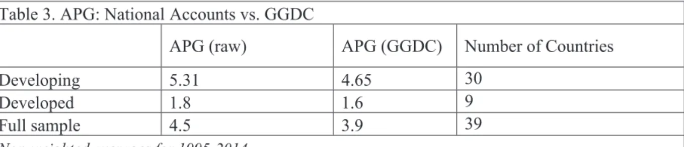
Table 3.
APG: National Accounts vs. GGDC
Table 4.
Working hours
Table 5.
APG and wage gaps
Table 6.
APG/AWG over time
Table 7.
APG adjusted for AWG and labor shares of income
Table 8.
Estimation of instrument: bilateral technology imports
Table 9.
Actual and predicted technology transfers
Table 10.
Basic panel OLS results
Table 11.
IV-estimation results
Table 12.
Alternative channels of technology transfers
Table 13.
Inclusion of related covariates
Table 14. Dynamic panel IV-estimation results
Table A1.
Summary statistics of variables used to compute APG
10 List of Figures
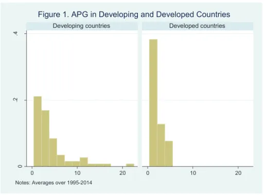
Figure 1.
APG in Developing and Developed Countries
Figure 2.
APG and per-person income
Figure 3.
Labor productivity gap relative to U.S.: non-agriculture vs. agriculture
Figure 4.
APG and agricultural employment
Figure 5.
APG and agricultural employment over time
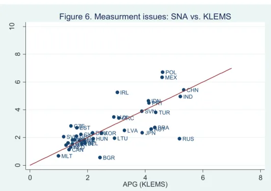
Figure 6.
Measurement issues: SNA vs. KLEMS
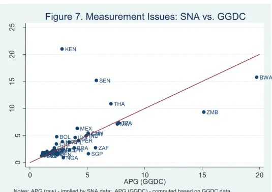
Figure 7.
Measurement issues: SNA vs. GGDC
Figure 8.
Hours worked in agriculture and non-agriculture
Figure 9.
APG and wage gaps – developing countries
Figure 10.
APG and wage gaps – developed countries
Figure 11.
Pattern of wage gap: non-agriculture and agriculture
Figure 12.
Revisiting the ‘Food problem’
Figure 13.
Trade and food exports
Figure 14.
APG and relative per-worker capital intensity
Figure 15.
Ratio of per-worker-capital in non-agriculture and agriculture
Figure 16.
Bias in technology transfers implied by data
Figure A1.
Labor productivity relative to U.S.L agriculture vs. non-agriculture
11
List of Key Abbreviations
APG – Agricultural Productivity Gap
CEPII – Centre d'Etudes Prospectives et d'Informations Internationales
CES – Constant Elasticity of Substitution
FAO - Food and Agriculture Organization
GGDC - Groningen Growth and Development Center
ISICV - International Standard Industry Classification
KLEMS - Capital, Labor, Energy, Materials, and purchased Services
OECD - Organization for Economic Co-operation and Development
SITC – Standard International Trade Classification
SNA - System of National Accounts
TFP – Total Factor Productivity
UNCTAD – United Nations Conference on Trade and Development
WDI - World Development Indicators
12 Introduction
As of 2013 average per-person income difference between the richest and the poorest 25% countries is recorded roughly 20-fold1 . This gap is largely reflected on sectoral labor productivities. Comparing to the rich group agriculture is 35-times less productive in the poor group, and the analogous gap constitutes the factor of 12 for non-agricultural sectors. Almost half of workers in the poor nations are engaged into agricultural production. These numbers blindly imply to the presence of significant cross-sector productivity disparities in developing countries, and more importantly, to the large portion of labor stuck in relatively unproductive sector. Other things being equal, there is nontrivial incentive for relocation of workers from agriculture into non-agriculture, which, in turn, should greatly lessen the income gap across nations.
Data from the National Accounts suggest that agricultural productivity gap (APG), measured as the ratio of per-worker value added in non-agriculture to that in agriculture, stands over the factor of 4 in developing countries with increasing trend over the last two decades. If they can earn more income in other sectors, why are the agricultural laborers not simply moving out of agriculture? Why are the significant potentials for income gains not being realized? This work intends to provide a complementary standpoint in addressing these questions that have been rigorously discussed in development economics literature.
13
In founding theories, relatively large productivity gaps in agriculture is attributed to differences in land quality, climate, and capital intensity (Clark, 1940), the ‘food problem’ (Schultz, 1953), as well as stagnant production technologies and human capital (Schultz, 1964; Hayami, 1969). Recent streams of literature have explored the role of capital market distortions, and resulting statistical discrepancies due to home production (Parente et al, 2000; Gollin et al, 2004; Herrendorf and Schoellman, 2012; Gollin et al, 2014); human capital differences across sectors due to skill-constraints and skill-intensiveness of production technologies (Caselli and Coleman, 2001), self-selection of labor based on observed abilities (Lagakos and Waugh, 2013), and on unobserved skills (Young, 2014); frictions distorting the labor markets (Restuccia et al, 2008; Au and Henderson, 2006; Munshi and Rosenzweig, 2016) as well as aggregate productivity inefficiencies (Caselli, 2005; Vollrath, 2009), and barriers for using intermediate inputs (Restuccia et al, 2008) to explain the sectoral productivity discrepancies in poor countries.
However, the half of the observed magnitude of APG as well as its increasing trend in developing countries has remained unexplained (Gollin et al, 2014; You and Juraev, 2017a; Juraev and You, 2017b).
This work proposes an alternative theory that complies with the observed magnitude and pattern of APG both over time and across countries. Specifically, we argue that puzzlingly large portion of the productivity gap in developing countries can only, and fully, be attributed to ratio of labor shares of income in agricultural to that in non-agricultural production. After using the data on labor shares corrected for self-employment, we show
14
that the puzzle profoundly disappears! More importantly, given unchanged pattern of wage gaps, moderately increasing trend of APG implies that labor shares are decreasing (increasing) in non-agriculture (agriculture) due to increasing (decreasing) shares of capital and technologies. In a simple accounting exercise, we demonstrate that relative sectoral capital intensities in the developing countries have remained constant, and thus, the changes in the productivity gaps unequivocally result from relative technical changes – more intense in non-agriculture comparing to agricultural sector.
In a simple formal framework with two sectors, two factors, and exogenous prices, we also show that in equilibrium, with constant labor supply, APG can be related to relative cross-sector technical change through skill-premium and division of, heterogeneous in skills, labor. Relationship is not positive per se without three empirically substantiated stipulations from literature. The first is the technology-skill complementarity hypothesis originating from Hicks (1932), which warrants a positive relationship between technical change, demand for skilled labor, and the skill premium. The second is the technical change that is sector biased resulting from demand driven profit incentives of producers. And finally, it is the aggregate technical change in developing countries that take place primarily through adoption of technologies from more advanced economies.
In our theoretical proposition, the skill-biased sector-specific technical change in developing countries via technology transfers increases the skill premium and allocates relatively more skilled labor into non-agriculture. Concentration of skilled labor further induces the technical change and the transformation of production technologies in the
15
modern sectors. Agricultural production, on the contrary, remains relatively sluggish and unproductive.
We test our hypothesis through two specifications of empirical estimations using the data for the sample of 153 developing countries for the period of 1995-2014. In the panel instrumental variable estimations, technology transfers are proxied by the imports of machinery and equipment classified under the Section 7 of the Standard International Trade Classification (SITC7) of the United Nation’s Conference on Trade and Development (UNCTAD). In order to overcome the issue of endogeneity, the imports are instrumented by the cumulative sum of bilateral trade of technologies predicted based on geographical factors and proximities among countries, and the innovative intensity of the technology exporters. The key exclusion restriction is the innovative intensity of the technology producers, measured as the ratio of aggregated R&D spending to GDP. Controlling for country specific fixed factors, panel instrumental variable estimation results provide plausible support for the proposition that technology imports are an important determinant of APG in developing countries. Findings are robust to inclusion of related covariates, sample restrictions, as well as factors representing alternative channels of technology transfers. In this first set of estimation specification, it is assumed that the R&D intensity of partner countries does not affect APG in developing countries except through technologies imported. The validity of this exclusion restriction is tested using the data on direct investment flows. However, due to paucity of complete data on other factors through which R&D intensity of the technology exporters may affect the sectoral productivities in
16
developing countries, and because the panel instrumental variable estimations do not take the possible dynamic prevalence of APG over time, estimation results may well be subject to debate.
To provide alternative evidence on the theory developed and account for the likely dynamic persistence of APG, the impact of technology transfers is also estimated using Arellano-Bond system dynamic panel two-step specifications, where all variables-in-levels are instrumented by lagged differences and variables-in-differences are instrumented by lagged variables in levels as in Arellano and Bover (1995) and Arellano and Bond (1998). Moreover, in order to directly control for the sectoral bias in technology transfers, the key variable of interest in the dynamic panel specification is measured as the ratio of non-agriculture specialized machinery imports to those specialized for agricultural production. Overall, the results from dynamic modifications suggest that 1% increase in the ratio of non-agricultural-to-agricultural technology imports tends to increase the productivity gap by 0.18 units. Entailing tests provide plausible support for the validity of the instruments used and the inferences derived.
This work fits into existing literature in number of ways. First, we demonstrate that intersectoral allocation of skilled labor is determined by relative technical change in non-agriculture and non-agriculture. In existing models e.g. Lagakos and Laugh (2013) and Young (2014) distribution of skills is solely a supply side decision, where the skilled self-select into sectors based on their observed and unobserved characteristics. Additionally, the formal framework in this paper distinguishes the aggregate productivity parameter from
17
sector-specific ones by formulating the production functions with skill-augmenting technical change in each sector. This formulation explains the relevance of the aggregate efficiency debated in Gollin et al (2004), Vollrath (2009), and Caselli (2005).
Using alternative sources of data, we also explore the relevance of statistical discrepancies and mismeasurement in calculation of productivity gaps for much larger samples than those in Gollin et al (2014) and Herrendorf and Schoellman (2012). Our findings reinstate that, while the magnitudes of APG’s in the sample of developed countries seems slightly overestimated than those implied by national accounts data, productivity gaps in developing countries cannot simply be attributed to the measurement issues. Contrarily, the measurement problems seem to be relevant in the empirical estimations of labor shares of income, which consistently assign lower values onto agricultural comparing to non-agricultural production functions.
Furthermore, this work presents a unique comparative analysis of economic transformation of the advanced countries from a historical perspective, which helps understand why the developed countries have exhibited low and relatively constant APG’s for over hundred years until now. The conclusions from the analysis imply that the historical development path of the advanced countries today did not necessarily embody large sectoral productivity disparities. Accumulated knowledge and human capital development triggered productivity growth, primitively, in the agricultural sector. Sufficiently high agricultural productivity enabled the reallocation factors of production and excess resources into non-agricultural sectors. The non-agricultural productivity revolution preceded the industrialization
18
stage in the case of the advanced economies. The sequence of transformation, however, seems to be reversed for the developing countries today due to the availability of the technologies readily available in the world markets.
Another important novelty of this work is the establishment of empirical link between technology transfers and the productivity gaps in developing countries. To the best of our knowledge, this is the first attempt to do so. The closest in context research to this work by Wang and Wandschneider (2014) presents two-sector small economy endogenous growth model and concludes that increase in product-varieties’ share in manufacturing imports increases the sectoral productivity in favor of modern productions. Their underlying intuition originates from Schumpeterian models of endogenous growth that increasing varieties in manufacturing imports induce the creation of more product varieties in the domestic manufacturing sector and increase labor productivities. They, however, assume that trade does not result in reallocation of labor, neither do they take the heterogeneity in skills of labor into account. Moreover, in their framework similar reasoning in case of varieties in agricultural imports would also give symmetric conclusions in favor of decreasing APG. In this work, we allow for technical change to be neutral, or non-agriculture biased, or non-agriculture biased. Should technical change favor non-agriculture relative to non-agriculture, skill premium would increase, and APG would decline due to relatively more skilled labor moving into agriculture.
Key findings from this work corroborate longstanding views that without technical change traditional agricultural production technologies deliver decreasing returns at increasing rate
19
(Theodore Schultz, 1953, 1964; Arthur Mosher 1966; Yujiro Hayami and Vernon Ruttan, 1985; Peter Timmer, 1988). High and increasing APG in developing countries suggest that the central importance of agriculture in development, at least in terms of the existence of large pools of less productive workers, seems yet to be tackled with proper development policies. Instead, surplus resources are directed to the productions in the non-agricultural sectors at the cost of delaying agricultural, perhaps aggregate, development.
Particularly, our analysis and results suggest that, in the short run, development policies ought to emphasize on the elimination of barriers to free labor mobility between agriculture and non-agriculture, or equally, rural and urban areas. In the long-run, governments should pay greater attention to technical change in the agricultural productions, whether through domestic development or adoption of appropriate technologies from more advanced countries. Accumulation of human capital in the economy, overall, would make more skilled labor available for both traditional and modern sectors to embrace technical changes more easily and consistently.
20
Chapter I. Agricultural Productivity Gap: Theory vs. Data
1.1. Preliminary Analysis
In this section, we start off by presenting the analytical discussion of labor productivity gaps implied by national accounts data. By definition, APG is measured as the ratio of value added per worker in non-agriculture to that in agriculture:
/ (1) / n n a a VA L APG VA L
Where, VA and L are value added and labor, subscripts ‘n’ and ‘a’ refer to non-agriculture and agriculture, respectively. ‘Agriculture’ includes agricultural production, hunting, forestry, and fishing in accordance with the International Standard Industry Classification (ISIC) Rev.2 of the United Nations2. Non-agricultural sector is composed of all other economic activities. Value-added is the difference between gross value of output and intermediate inputs, and available from the World Development Indicators (WDI). Labor is derived from share of employment in each sector and total employment in the economy. Data on the share of employment is available from Food and Agriculture Organization (FAO) of the United Nations3. Total employment is measured by the total number of persons of 15 years of age or older engaged in any economic activity for a given year. Number of persons engaged is obtained from the World Penn Tables. Sample ranges from
2Equally refers to Sections A and B in ISIC Rev.3 and Section A in ISIC Rev.4.
3FAO employment shares data originate from the International Labor Organization’s (ILO)
household survey data. Surveys that are concentrated on non-representative geographical coverage such as urban areas, towns, major cities, and state-owned enterprises are excluded.
21
1995 to 2014 and includes 176 countries with relevant data available. Summary statistics of the variables presented in appendices Table A1.
Countries are classified into low income, lower-middle income, higher-middle income, and high-income categories in compliance with the 2016 December review by the World Bank. It is important to acknowledge that there is no precise definition of the ‘developing’ and ‘developed’ countries. Frequently, ‘high-income’ is interchangeably used to represent the ‘developed’ group despite there is significant heterogeneity in quality of economic development4. To tackle this issue, economies that became OECD member in or before 1995 are conditionally referred to ‘developed’ countries5. Table 1 summarizes the APG’s computed6.
Results imply that an average worker in non-agriculture is over four times more productive than her counterpart in agricultural sector in developing countries. The calculated gap is two-fold in the developed countries. When population weights are applied, gap further increases in the sample of low and middle income or, in general, developing countries. This implies that APG is relatively larger in countries with more population. On the contrary, weighting decreases the gap in both high-income and developed countries.
4For example, it would be implausible to treat Saudi Arabia and Sweden, or Croatia and Canada
under one level of development.
5Following countries are classified into the ‘developed’ group: Australia, Austria, Belgium, Canada,
Switzerland, Germany, Denmark, Spain, Finland, France, the United Kingdom, Greece, Ireland, Iceland, Italy, Japan, Luxembourg, Netherlands, Norway, New Zealand, Portugal, Sweden, and the United States.
22 Table 1. Implied APG
Country groups APG Weighted APG Number of
countries
Low and middle income 4.03 4.5 121
High income 3.01 2.8 55
Developing 4.2 4.3 153
Developed 2.2 2.1 23
Notes: The second column is APG simply averaged over 1995-2014. The third column is the average of population weighted APG over 1995-2014.
Among the developing countries the largest in magnitude productivity gaps are recorded in Bhutan (15.1), Botswana (15.8), Qatar (22.5), Kenya (21), and Senegal (15.2). Calculated APG’s in developed countries are, roughly, in the range of one to five. Median APG is 3.1 and 1.8 in the ‘developing’ and the ‘developed’ samples, respectively. Distributions are illustrated in Figure 1.
Is high APG associated with low income? The answer seems to be mixed. Figure 2 illustrates the raw APG and purchasing power adjusted income per-capita. The observations from the figure has two important implications: that for same or similar levels of income, APG varies significantly, and that for same or similar levels of APG, income differences can be enormous. For example, both Tanzania and Senegal have per-person income of roughly 1700 USD. The productivity gap is 7.4 in Tanzania whereas it is 15.2 in Senegal – the difference is twofold! On the contrary, comparison between Guinea and Trinidad and Tobago shows that both have APG’s slightly over 10 whereas the income difference between the two is 22-fold! However, in general, higher income is associated with lower APG’s.
23
Negative, yet blurred, relationship between APG and income can be observed due to two reasons: 1) because a nontrivial part of income is determined by other factors; 2) because APG by itself does not necessarily imply to having a low level of income. By no means we neglect the importance of other factors, yet, continue with the second reason to keep the scope of this work as focused as possible. Since APG measures the relative productivity in two sectors, a country with high APG can have high income if: a) both agricultural and non-agricultural labor productivity is high relative to other countries; or b) unproductive agriculture employs small portion of labor force; or c) both. Opposite notion holds for countries with low implied APG and low income. High APG in countries with large share of employment in agriculture, however, implies to substantial potential gains in reallocation of labor from the less productive to the more productive sectors. In order to provide more substantiated explanation to the importance of sectoral productivity
0
.2
.4
0 10 20 0 10 20
Developing countries Developed countries
Notes: Averages over 1995-2014
24
disparities it is of crucial importance to look at the share of employment in agriculture as well as labor productivity in both sectors relative to an arbitrary cross-country threshold level.
As a threshold level, we choose the labor productivity in the US, without the loss of generality. Figure 3 compares the labor productivity gap in non-agriculture and agriculture in different groups of developing countries. Specifically, vertical axis represents the ratio of non-agricultural labor productivity in the US to that in each country. It, therefore, measures how unproductive an average non-agricultural labor is comparing to her counterpart in the US. Horizontal axis represents the ratio of agricultural labor productivity in the US to that in each country. For example, factor of 10 on horizontal axis means that average agricultural labor is 10 times more productive in the US comparing to average
0 5 10 15 20 25 APG 6 8 10 12 log(per-capita income, PPP)
Note: Empty and filled circles represent developing and developed countries, respectively. Averages over 1995-2014. Figure 2. APG and per-person income
25
agricultural worker in the country of interest. Measures of labor productivity are adjusted for Purchasing Power Parities (PPP) in each country and represent face values.
Conclusions from the Figure 3 are striking7! In almost all developing countries, labor productivity gap relative to the US is greater in agriculture than non-agriculture. For example, in Ethiopia, agricultural labor is 64 times less productive than that in the US, whereas the gap is 18-fold in non-agriculture. The relative gap in agriculture reaches shockingly large level of 121 for Mozambique, while the same gap in non-agriculture stands at the factor of 15.
Similar picture is observed in case of middle-income countries. In China, for example, labor is 36-fold less productive in agriculture, whereas the gap is 3.6 for non-agriculture relative to the US. The gaps are 2.8 and 1.8 in agriculture and non-agriculture in Korea, respectively, and 23-fold and 6.5-fold for India.
All these numbers imply that high agricultural productivity gap is due to very low labor productivity in agricultural production rather than very high non-agricultural productivity in the developing countries.
7 The same picture for developed countries is presented in Figure A1 in appendices. I let that
26
Now, let us return to the motion about the relationship between APG and per-person income and present two extreme cases. Consider Central African Republic (CAF). CAF is one of the poorest nations in the world with per capita income being around 800 USD. However, APG in CAF averages to 1.8 over 1995-2014, which is even lower than the average corresponding to the developed countries in Table 1. Coexistence of low income and low APG means that in both agriculture and non-agriculture labor productivity is proportionately low. Indeed, referring to the low-income group (3) in Figure 3, relative to the US, labor productivity gap in agriculture and non-agriculture is 44 and 39 – equally low. Consider, now, Qatar. In Figure 1, Qatar is the obvious outlier with APG over 20 and
UGA UGA GNB AFG MOZ MLI SEN BEN ETH CAF ZWE CAF CAF BDI CAF TCD UGA GNB BDI GNB RWA RWA SEN TZA RWA MWI ZWE TCD COM COM AFG MLI COM TGO ERI NPL MDG AFG TZA NERRWA
MOZ COM BFAUGA TCDGNB SLE MLI TGO NPL SEN ZWE SLE NER MWI RWA ERI COM CAF ERI ERI BDI CAF RWA GNB ETH ZWE TZA ETH ETH ETH UGA GNB MDG SLE MLI COM SEN TZA MWI BDI SEN NPL COM SEN MOZ TCD RWA MDG COM SLE GMB GMB GMB GMB GMB GMB GMB NER GNB NPL SLE MWI BEN TGO COM ZWE COM BEN GMB ETH GNB COM COM ERI BFA BFA AFG BDI MDG NPL GMB MWI RWA SEN NER GMB ETH MLI ERI SEN ERI MWI TCD MLI NER TZA TCD SLE AFG GMB ZWE NER AFG AFG GMB ETH MDG NPL NPL NPL ZWE CAF UGA TGO CAF BEN UGA BFA NERERI ZWE CAF UGA COM CAF BFA SLE TZA BDI ERI AFG TGO TZA UGA TGO TGO TZA CAF NPL ERI ZWE TZA ETH CAF MWI CAF MOZ BEN MDG COM MDG BEN MDG MDG BEN TCDGNB BFA SEN MDG UGA MLI MLI MLI MDG SEN NER NPL ZWE RWA ETH TCD BEN ZWE RWA MLI MOZ MOZ ETH TGO NPL MWI TZA AFG NPL MWI MWI GMB ERI ETH BDI SLE ERI BFA SLE BDI BEN BDI NER TZA NER ETH BEN CAF ERI MLI BFA MWI GNB MOZ AFG CAF NPL NPL RWA BENNPL GMB BDI SEN MLIGNB AFG RWA GMB GNB MDG NER GNB ETH MLI TCD MLI BEN MOZ BDI NER BFA ETH ETH GNB MDG MOZ COM UGA TCD NER AFG GNB ERI MWI TZA MOZ MWI SLE RWA GMBTZA TCD TCD CAF BFA MOZ ETH RWA SLE RWA RWA RWA GNB COM AFG SEN MLI SEN TZA TZA MLI RWA MOZ ERI SLE MLI SLE SLE SLE ETH SLE ERI SLE SLE MOZ BFA RWA SEN NER BFA MLI NPL MDG TCD NER UGA MDG GMB SEN ZWE ERI SLE ZWE GNB UGA CAF GMB NPL MDG COM BFA TCD COM TCD BEN MLI BFA TGO MWI TGO TGO TGO TGO NPL NER AFG TZA GMB SLE MDG UGA CAF MOZ AFG TCD BDI BDI BEN TZA SLE TCD COM UGA UGA BDI UGA UGA MWI TCD CAF MOZ NER SEN ETH TCD MWIERI AFG BDI MWI TCD MOZ GNB ERI TGO BDI TZA BEN TGO MLI MWI UGA GNB TGO RWA BDI MDG CAF ZWE ZWE ZWE ZWE ZWE TGO ZWE CAF ETH ZWE TGO ZWEMDG MOZ COM MDG MLI ETH BEN TGO BEN BFA BEN GMB BEN SEN BEN GNB MWIMWI TZA SEN NPL
AFG TZA NERRWA ERI NER TCD UGA BDI MOZ ERI MOZ BFA BDI BFA BEN BDI MDG SEN NER TGO GMB GNB COM AFG AFG MWI TGO NPL BFA SEN NPL MOZ AFG AFG UGA SEN MOZ TZA BFABFA NER
BDI BFA 0 10 20 30 40 0 50 100 150 Low income (1) PHL SDN MMR UZB LKA KEN UZB GTM BTN EGY PAK TJK MAR KEN NGA KEN MNG VUT KHM PNG ARM KHM ZMB MDA VNM PAK KEN VNM KGZ PAK TUN BOL MMR SLB TJK SLBIND PHL STP SWZ BTN VUT YEM PHL TJK BTN LKA SDN CIV NIC GHA SWZ EGY MMR UKR TJK ZMB CIV TJK STP MMR GHA BGD HND LAO KHM TUN UZB SLB TJK SWZ NIC COG SWZ BTN COG PAK UKR LKA TJK COG UKR SWZ PHL SLB NIC BTN PAK SLV MAR CPV PAK LAO MMR KGZ PNG MMR ZMB GHA BGD KGZ IND YEM BGD SLV GHA PHL VUT STP MNG SWZ SLB MNG HND PHL CMR MNG KEN MMR MAR CMR MNG CIV GTM MDA MNG ARM MNG SLB PNG MNG HND SLB SLB EGY TJK PAK IDN SLB TJK STP GTM SLV MNG CIV SWZ LSO ARM VUT CPV PHL CPV SLB VNM PNG MMR KGZ STP BGD TUN UZB EGY EGY COG IND TJK GTMIDN MRT SWZ YEM KHM SLV NGA LKA GTM MRT UKR LSO CMRBGD UKR ZMB BOL PNG ZMB PNG ARM LAO LSO SDN LSO BTN SWZ SLV LKA UKR GHA VNM GHA BTN IDN BGD UKR ZMB CIV BTN SLV SLV TON MRT VUT VUT GHA YEM IDNYEM KEN IDN SLV MAR BGD PNG NIC NGA BTN TON UKR PAK NIC GHA CMR STP HND COG TON CMR GTM TUN TON ZMB CPV NGA SLV GTM SLV GHA GTM TON TON IDN SDN NIC TUN TON TON BOL TON UKR TUN LSO TUN TUN CPV BTN LAO PAK LSO KHM HND LSO IDN GHA SLB SDN YEM YEM GTM KGZ EGY MDA BTN SDN PHL GTM HND BTN SDN MRT MDA TON MDA HND LAO UKR SLB MDA CMR EGY BOL PHL CPV GTM MRT UKR EGY HND KEN MNG TJK GHA MMR YEM ARM TUN GHA TUN HND LAOIND YEM LKA KGZ KGZ MDA BOL SLV LSO MAR UZB TJK PNG MAR VNM PAK TJK IDN MMR IDN UKR IDN SWZ IDN TUN IDN IND SDN HND MNG GTM MRT LSO NGA BOL TJK SDN IND MDA IND TON MDA VNM CPV KEN IND BGD LSO SLV KHM IND LKA BTN BGD EGY MDA NIC LKA LAO MNG KHM HND UZB LAO MDA IDN MMR PNG GHA BGD KGZ YEM ARM PAK MAR YEM STP KGZ VUT PHL KGZ TUN STP MDA NIC NIC STP CMR GHA IDN KHM MAR ARM MMR STP KEN BGD GTM STP LAO STP MDA STP VUT KHM LSO KHM TON NGA PNG CMR UKR KHM LAO PHL LKA KHM HND IND IND LSO PNG PHL MNG MRT IDN LKA NIC BOL NIC GTM CPV YEM CIV KHM SLV STPZMB EGY ARM ZMB CMR YEM IND KGZ BGD PHL CPV ZMB GTM ZMB SDN GTM COG VNM LAO TJK MNG EGY MAR CIV UZB ARM GTM BGD MRT MAR VUT UZB HND KGZ UKR LSO MAR KHM BGD SLB LKA LSO CMR KHM NIC IDN PNG NGA COG BTN SWZ VUT MRT MDA MMR MRT MRT LAO MAR CIV KEN COG LKA KGZ EGY KEN EGY PAK COG LKA TUN NGA BOL YEM MNG MMR MRT CMR BOL UZB IND TUN KEN PAK UZB CMR KEN BGD STP TUN ZMB SDN VUT EGY HND VUT VUT PHL COG KHM KEN MAR YEM CIV TON IND NGA EGY COG STP CIV TON VNM LAO KHM BOLIND TJK CIV VUT COG PAK COG PAK PHL TJK CIV SDN IND PNG EGY COG VUT VNM TUN IND ARM EGY CPV YEM PNG SWZ BOL BTN MDA SDN CPV CMR MDA GTM PHL BOL KGZ VUT IND KEN VNM LKA TON MNG MNG LAO VNM PNG STPZMB CIV YEM SLB UZB LKA MNG VNM CPV CIV SWZ SWZ IND CMR BOL TONCPVCPVCPV UZB BOL LKA VNM VNM MNG PHL CMR GHA GHA MNG NGA KEN CIV TON UZB KHM STP BTN TUN HND SLVIDN LSO TJK ZMBCOG GHA NGA PAK MAR MAR UZB KEN UZB KGZ ARM SLV PHL PNG UKR MRT VUT IND SLB LAO EGY PNG NIC BOL KGZ SDN ARM HND ARM CPV TON CIV VNM NIC SLB MMR PNG BGD MAR CIV ARM UZB MMR MMR CIV PNG TON BGD PNG VNM TON TUN COG BGD NGA SWZ MMR ARM UZB KHM KHM BGD BGD LSO MMR LAO SWZ ARM PAK STP TUN MDA CMR BOL TON BTN KGZ IDN PHL ZMB SWZ COG MMR LAO YEM STP MRT HND KEN MNG YEM CIV SDN VUT PNG LAO BOL IDN KGZ NGA CMR KHM STP NGA TJK SDN TJK UKRCPV CIV MDA HND NGA VUT SWZ COG LSO SLB CMR MDA NGA SDN BTN GHA CMR PHL MDA BOL KEN SLV LAO KEN MRT VUT SWZMRT VNM ZMB BGD LSO UKR MAR SDN SDN SWZ SDN SWZLKA SLV GTM UKR BTN PAK LAO UKR UZB BOL VNM KEN PAK IDN SLV CPV BTN SLV GHA MRT CPV SLB ARM VNM SLV ARM UKR EGY BOL PAK MDA HND UZB LSO NIC LKA SLB KGZ NIC GHA MAR KGZ LAO ZMB BTN EGY CMR CPV TUN MRT CMR MRT COG PAK PHL MRT LKA EGY ZMB NGA VNM UZB LKA IND IDN ZMB MMR NIC SDN HND KGZ NIC NIC SLB GHA ARM GTMYEM COG VNM NGA SLB UKR CIV NGA BOL LKA MRT CPV MAR MAR HND LSO UZB MARSLV YEM ARM ARM NGA LSO COG NGA NIC ZMB TJK NIC GTM ZMB TUN VUT 0 5 10 15 20 0 20 40 60
Lower middle income (2)
NAM CHN JAM DOMJAM MYS MYS GEO ZAF BRA IRN JAM CHN MKD THA SRB KAZALB CRI MDV THA SUR BRA BLZ CUB COL TUR BLZ LBN DOM GUY TKM RUS PER LBN AZE CHN DZA JAM ARG TKM NAM CHN THA GEO SRB BWA RUS COL KAZ JAM BLZ SURCUB VEN ARG AGO VENSUR BIH AZE CHN LBY CHN DZA MDV BLZ CHN CHN ALB VEN SRBTUR SUR AGO BIH MKD PER THA DOM CRI LBN TKM COL PRY LBN CRI PAN IRN BLR PRY ALB PAN VCT VENJOR LCA ALB ZAF LCA ALB PER SRB LBY GUY LCA ARG ECU PRY CRI MKD BLZ LCA FJI ZAF MKD ALB GEO CUB LBN TUR MEX NAM JOR LBY PRY AGO LBN GNQ DZA LBY GAB BRA ECU IRN LBY BGR PRY PER VCTLCA MKD RUS SUR THA BLR GEO PAN BRA SRB SRB SUR LBY SRB JOR BLR TUR BIH MKD VEN AGO ARG SRB JORNAM BRA AGO BGR LBN AZE CUB BGR GUY PAN COL ARGJOR BIHKAZSUR THA
TKM FJI SUR BGR GAB CUBCRI COL GUY BRA JOR KAZ PER JAM BIH PAN BLR ZAF BWA PAN AGO VEN MUS ARG GAB SUR GNQ BRA TKM LBY NAM MKD FJI CUB LBN JAMPER VCT BGR BRA GNQ CRI TKM BLZ PER TKM LBN IRN LCA FJI MDV GEO LCA MDV IRN MEX ZAF VEN LCA GAB GAB MYS RUS MYS RUS RUS GEO BIH JOR MEX KAZ JAM PRY ARG ALB RUS PER PRY GNQ GEO MUS MKDECUVCT CHN ZAF VCT DOM BLZ BRA MKD TUR LCA PAN BIH ZAF MKD MKD MKD MDV JAM ARG VCT GNQ DOM ZAF COL BRA ZAF PRY VEN BIH TUR MUS LBY PER SUR SRBVEN GAB BWA MDV MUS TKM AZE ARG CRI VEN LBY CRI ECU BIH AGO PAN BWA FJI MYS DOMCOL BWA THA TUR ARG TUR ALB BWA PAN CRI BGR NAM RUS GAB ALB AZE MYS BGR DOM LBN PRY KAZ DOM DZA MEX PER ALB PAN BLZAZE CRI AZE GNQ AZE DZA MDV DOM IRN MYS GUY TUR VEN MEX MUS ECU NAM VENKAZ ARGSUR GAB NAM LCA NAM PAN COL TKM BRA KAZ GAB NAM ZAFNAM MEX ECU ECU TUR LCA AZE MYS THA MUS MYS PRY GUY PER MUS MUS SRBMYS ECU MYS AZE MKDBRAECU MKD RUS AGO CRI BIH PAN LBY ZAF LBY VCT DZA DOM AGO COL AGO GUY MYS GUY JOR MDV PER CRIFJI ECU MUSRUSBRA LBNSUR THA LCA TUR ALB CHN CRI MEX BWA DOMVCT ARG GEO AZE TKM AGO MKD CUB DOM BWA LBY KAZ BLZ SRB MEX PER DZA KAZ BIH JAM ZAF TKM JAM GNQ GNQ GAB BLR KAZ VCT LBN IRN PRY FJI BIH DZA GEO AZE CUB ECU LBN DZA SUR COL LBY MDV GUY KAZ DOM MYS IRN BGR MUS ZAF RUS AZE GEO GAB GAB MEX GNQ BIH DZA VCT JOR TUR MDV AGO CRI GNQ MUS AGO LBY GNQ CUB CHN COL FJI CUB GEO COL MKD ZAF BGR AGO SURCUB FJI COL GEO LBY BLZ TUR THA GEO CRI BIH CRI MYS CUB GAB GAB SUR GUY NAM GAB TUR ARG LCA BLR MDV GAB ECU CUB JAM IRN BGRCOL CUB TUR GNQ VEN NAM BLR NAM AZE JOR FJI CRI DOM AGO AZE IRN AGO VEN MKD MYS JAM ARG GUY FJI FJI JOR FJI GEO ECUFJI MYS KAZ FJI FJI BWA THA DOM CHN IRN GNQ MEX SRB SRB THA BLR TKM SRB VCT COL GNQ VCT CRI GUY MEX TUR IRN DZA JAM JAM DOM ARG PER
JORNAM THA LBN DZA MYSJOR NAM PRY BLR ARGVEN ALB BLZ CUB BIH BIH BLR GNQ AGO VCT PER ECU GNQ BGR SRB TKM TKM ARG MKD RUSBRA ECU GUY ECU ZAF IRN BGR ARG PRY PRY ECU PER CUB AGO DZA VEN RUS LCA TUR AZE GUY MEX IRN KAZ THA DZA VEN VEN DZA VEN AGO DOMJAM MEX ECUDOMDOMDOMVCTVCTVCTVCT
SRB MUS TUR VCT BRA BLZ RUS GEO MDV BLZ ZAF BLZ ECU TKM MDV MUS VEN MUS AZE MUS PRY ALB BLZ CRI KAZ BGR THA BIH CHN FJI MEX LBYTUR LBY MKD GNQ MUS LCA MUS SRB GUY BWA SUR MDVLCA FJI LBN BLZ BRA LCA BWA MDV LBNJORPAN CUB THA THA TKM BLR CUB ARG GNQ NAM MUS LBN GNQ RUS THA JAM KAZ DZA JOR ALB AZE JORZAF JAM FJI JAM BGR GNQ ZAF BLZ ZAF BRAFJI IRN DOM GUY
SURNAM BWA RUS KAZALB GEO PER BRA MDV PER PRY BLR DZA RUS LBY ALB ALB JOR BLR ALBMDV BGR GAB SRB LBY NAM CHN RUS DZA GUY GEO GEO BRA ALB MUSRUS BLZ VCT BIH BRA JAM MKD PRY LBN MUS ECU GNQ SUR IRN BGR GEO CUB GUY MEX COL GEO LCA KAZ SRB COL KAZ MKD MEX PANMEX FJI VCT DZA BLR IRN MDV BGR PAN GAB TUR PRYTKM BGR PRY BWA MYS TKM LCA BLR ARG NAM TKM LBN TKM JOR JOR BIH AGO CUB BWA THA SUR DZA TKM LBN BWA GUY ARG CHN MYS BIH THA SRBDZA RUS LCA BGR LBY BWA KAZ SRB RUS BLRCOLAZE CRI MEX AZE CHN IRN BGRBLR MYS PER GEO PAN COL BLR JOR BWA PER BRA BLR CHN BIH CHN BWA CHN KAZ BLZ SUR BLR ZAF LCA ZAF GUY MUSALB GAB GAB AGO GAB BWA PRY JAMPER IRN LBYIRN COL SUR BWA COL BGRBLZ ECU CUB PANMDV PAN VEN ALB PRY BWA LBN AZE
JORMEX THA MDV BLR PANMEX PAN BLZ MEX GUY MDV CHN IRN MYS TUR CRIVCT NAM PAN CHN 0 2 4 6 8 0 20 40 60 80
Higher middle income (3)
POL SGP CHL BHR LVA BRN CZE LVA SAU URY BHS HUN BHRCYP HUNLTU BRN TTO SVN BHR BHR QAT SAU BHS POL QAT KOR LTU QAT BHR URY QAT OMN SAU SAU TTO QAT SGPBHR SAU KOR SAU MLT MLT URY BHR OMN BHS KOR SVN TTO URY QAT CZE SVK SAU URY URY CYP OMN BRN KOR SVK BHS SGP SGP MLT KWT TTO BHR SGP SAU BHS CYP BRN QAT OMN SGP HUN SAU CZE SVN KWT LTU BRN HKG CHL HRV TTO CHL TTO URY KWT SVK TTO BRB KOR LTU TTO LTU BRB LTU MLT HUN SVN OMN KOR MLT URY BRN CZE BHS SVN SAU SAU SVK SAU EST SGP SGP BHS SGP CZE BRN KOR CYP TTO LTU POL MLT CZE CHL SAU EST LVA HRV SVK KOR KOR TTO BHS HKG SGP URY URY HUN BRB SAU KOR TTO HUN KWT HKG HKG OMN SVN EST SVN BRB EST BHS EST POL BRN EST POL BRB KWT POL BHR POL QAT BRB BRN SVK QAT HUN CYP URY CYP SVK QAT OMN HUN OMN OMN OMN HRV OMN OMN URY CYP BRN BRN HUN SVK BRB LTU HRV LVA CHL LTU MLT OMN HRV TTO EST OMN LTU POL SAU TTO SGP SVNHRV CZE SGP KOR MLT MLT LVA CHL HUN HRV KWT SVK SVN POL EST HRVBHS BRB MLT MLT TTO MLT MLT KWT SVK BHS QAT BRB URY SGP CZE SVN KOR CYP URY BRN CZE SAU BHR POL HUN CZE EST POL HKG BHR HRV SVN QAT KOR QAT HUN LVA HRV LVA LVA LVA LVA SVN LVA LVA MLT HKG MLT BRB CHL QAT KWT LTU LTU HRV QAT LVA TTO BHS CHL CYP CHL KWT POL BRB
HUN POLPOL SVK HKG OMN SVK MLT OMN LVA CHL CZE QAT KWT SVN KWT KWT HUNLTU OMN QAT KOR SAU CHL QAT KOR KOR HUN KWT HRV CHL LVA HRV CZE HKG LTU EST KWTQAT HUN HRV POL SGP TTO HRV KWT CYP POL BHS URY HRV SAU CYP CZE CZE SVN CHL KWT SVK SVN LTU KOR HKG BHR HUN URY CZE QAT EST LTU HRV BRN BHR HRV OMN BHS KOR MLT SGP HKGHKG BRB HKG HKG HKG BRB BHR HKG MLT HUN CYP SVK BHS TTO SGP BHS LVA KWT CYP BHR BRN OMN HUN KWT SGP POL TTO URY LVA LVA LVA LTU SVK BHR EST TTO CHL CYP SAU HKG LVA BHS CYP POL BHS KOR HRV CYP SVN SVK BRB LTU BRB HUN EST EST QAT SVN KOR KWT MLT SVKCZE BRN BHS SVKSVK EST POL HRV MLT SVK HKG CHL KOR SGP SVNHRV EST EST BHR BRN SVKCZE CYP CZE CYP CYP CYP CZE POL HKG EST HUN BHSLTU KWT HKG LVA BHR URY SAU SVN CHL BHR BHS POL URY CZE LTU KWT SGP TTO HKG SGP EST CZE SVN URY TTO CHL BRB OMN BRB CHL CHL CHL EST SGP CYP SVN SAU LTU EST OMN BRN BRB BHR BHR URY BRN CHL BRN BRN BRN BRB MLT BRB BRB HKG 0 1 2 3 4 0 5 10 15
High income, developing (4)
Note: Vertical axis=non-agriculture, horizontal axis=Agriculture.
Straight line from the origin represents the gap in two sectors being equal.
27
per-capita income being higher than that in all developed countries. What the case of group (4) in Figure 3 implies is that while Qatari agricultural labor is twice less productive than that in the US, non-agricultural labor is twice more productive than that in the US. In what we discuss next, less than 1% of the workers in Qatar are employed in agriculture, which allows for the existence of high APG and high-income (Figure 4).
Is there significant misallocation of labor? To address this question let me start off with the case of developed countries. In the ‘developed’ group, on average, non-agriculture is 2.2 times more productive than agriculture, and merely 4.7% of the employed are engaged into agricultural work. Without any assumptions, basic reasoning implies that even if some of the labor moved out of agriculture into non-agriculture the potential gain in aggregate productivity, or equally income-per-worker, would be negligible. On the contrary, in the case of developing countries, over one-third of the workers are in agriculture when the non-agriculture is over four times more productive. It is, therefore, plausible to expect that, holding everything else constant, reallocation of labor from less-productive sector to more productive sector should result in substantial improvement in per-person income in developing countries.
28
In fact, potential gain should be higher, the higher the implied APG and the higher the share of employment in agriculture. For majority of developing countries data displayed in Figure 4 show that higher productivity disparities across sectors are associated with higher shares of employment in agriculture. When the sample of 40 poorest countries is considered, share of employment averages to 70% in agriculture, and APG surpasses the factor of 7!
Have countries realized such potentials for income-gains? What stylized facts in Figure 5 imply is astonishing: despite the share of employment in relatively less productive sector – agriculture, has steadily declined over time, APG has increased in developing countries
SEN CAF MLI GMB LBR NER ERI SLE TZA ETH BEN GNB NPL RWA TCD MOZ UGA MDG AFG TGO ZWE MWI BFA BTN VUT KEN NIC COG MAR PAK IND SLB MNG SWZ TUN LSO YEM SLV MMR IDN SDN BOL WSM HND MDAKGZ KHM SYR GTM CMR NGA EGY MRT STP LAO TJK ZMB VNM GHA TON PNG BGD PHL CPV UKR LKA CIV UZB ARM THA BLZ GEO CHN CRI PER PAN JOR LCA ZAF MUS LBN MDV NAM BRA MYS MKD RUSSUR BWA KAZ MEX CUB IRQDOM FJI SRB VEN BLRGUY ECU VCTAZE ARG JAM PRY ALB GAB LBY DZA IRN BGR TUR TKM BIH COL CZELVA URY BHR SVN MLT BRN HUN EST POL OMN HRV TTO ARE NCL SAU QAT SVK HKG SGP KWT BHSBRB KOR CYPLTU CHL 0 5 10 15 20 25 AP G 0 20 40 60 80 100
Agricultural employment, (% of total)
Developing countries USA CHE NLD PRT AUT AUS SWE CAN IRL NOR LUX ITA GBR GRC NZL JPN FIN ESP BEL DEU DNK ISL 1 2 3 4 5 0 5 10 15
Agricultural employment (% of total)
Developed countries (averages over 1995-2014)
29
over the last two decades! On the contrary, there is no viable trend of APG observed in developed countries8.
What causes such a large magnitude of productivity disparities in developing countries? As countries develop, why have the potential gains implied by APG increased instead of decreasing? Why should we see APG even in developed countries at all? These are some, but not all, of the important questions that have not found complete answers in development economics research. This work is obviously not the first one to pose these inquiries. Related
8 In construction of the Figure 5, only those countries with complete data available from 1995 to
2014 are considered. Therefore, ‘developing’ and ‘developed’ samples include 116 and 19 countries respectively. 0 10 20 30 40 2 2. 5 3 3. 5 4 4. 5 1995 2000 2005 2010 2015
APG (Developing countries, left axis) APG (developed countries, left axis)
Agricultural employment (developing countries, right axis) Agricultural employment (developed countries, right axis)
30
literature can be traced back over a half a century. Yet, this paper intends to provide a complementary explanation to the puzzle.
1.2. Existing Literature
Before we move onto exploring the literature related to productivity differences in agriculture and non-agriculture, introduction of some basic accounting identities would be plausible. Referring to equation (1), labor productivity in each sector is as the ratio of value added (VA) and labor (L). As defined in System of National Accounts (SNA) of the UN, value added is the value of output less the consumption of intermediate inputs. When considered from the income approach, VA is the sum of labor’s and capital’s compensation:
(2)
VA wL rK
Where, ‘w’ and ‘r’ are wage-per-worker and rent-per-capital, respectively. ‘L’ and ‘K’ stand for labor and capital, as commonly expressed. Straightforward reformulation of (1) using (2) gives another representation of APG:
(3) n n a a w rk APG w rk
Where, k=K/L is the capital per worker in each sector.
Equation (3) implies that relative labor productivity in non-agriculture can be higher if wages and/or capital-per-labor are higher in non-agriculture, given that return to capital is
31
identical in both sectors. Existing literature can be precisely summarized around the equation (3).
Large productivity differences between agriculture and non-agriculture, both within and across countries, were first discussed by Colin Clark in his ‘The Conditions of Economic Progress’ in 19409. Clark, by analyzing extensive raw data, concludes that per-worker cereal production i.e. agricultural productivity was surprisingly lower in poor countries, and that low agricultural productivity was one of the key reasons for their high poverty rates. Holding the terms of trade between cereals and dairy products constant at 1925-1934 prices, he finds that merely 6.4 percent of the labor force in New Zealand would be enough to produce the dairy food requirements in the country. On the contrary, agricultural productivity was so low in former USSR that it would take twice the size of all labor force to meet the same limits. Clark suggests that differences in agricultural labor productivity can be, mainly, explained by land quality, climate, and relative capital intensities. Some of the views of Clark (1940) oppose those from later works such as Theodore Schultz (1964). Schultz neglects the importance of factor endowments and land quality, and asserts the role played by innovations, fertilizers, and machinery in explaining the productivity differences in agricultural sector between poor and rich countries.
Yujiro Hayami (1969) made one of the early attempts to quantify the Schultz propositions. Hayami, as in Clark (1940), also presents that for 1957-1962 years, India’s labor
9 Colin Clark is, in fact, one of the co-founders of division of economic activities into sectors:
32
productivity in agriculture was substantially lower than that in the US and Japan. More precisely, the gap was almost 50-fold between India and US, and 5-fold between India and Japan, when agricultural value added per male worker was considered. To decompose the gap, he estimates the world aggregate agricultural production function using data for 38 countries. Hayami finds that factor endowments i.e. land/labor ratio and fertilizers each explain 20% of the gap, whereas education, and research and development account for the remaining portion10. In case of India vs. Japan, human capital accounts for 40% of the labor productivity gap in agriculture. Hayami (1969) points out that India’s agricultural output would double if the level of education improved to Japanese level11.
Early analyses by Clark (1940), Schultz (1964), and Hayami (1969), among many others, are of absolute importance in terms of setting the cornerstones in APG literature. However, they are raw in a sense that the quality of data used is low, that scope of samples is limited, and that available theories and analytical techniques used are primitive.
10Hayami measures education as literary ratios and school enrollment ratios for the first and
second levels of education. The variable ‘research and development, and extensions’ is measured as average number of graduates from agricultural faculties in third level of education during 1958-1962 per 10.000 farm workers. (Hayami, 1969.p.3).
11Hayami’s (1969) conclusions are strictly based on the factors of elasticity estimated in aggregate
production function. Without doubt his work is of high importance in APG literature, however, certain assumptions and measurement issues in his calculations create grounds for flaw. For example, he measures the labor in agriculture as number of male workers in agricultural production. He also excludes the number of workers in forestry and fishing as he estimates the production function for crop-production only. Because of data unavailability, measure of agricultural output does not take the capital formation and capital stock into account, which may result in biased results. Such restrictions impose some critical doubts on estimated factor elasticities of production, hence, his concluding findings.
33
Subsequent works explaining the magnitude and importance of APG can be classified into three mutually nonexclusive categories. The first category includes the literature dealing with statistical discrepancies and measurement issues in computing the APG. There is a rationale doubt in development economics about the quality of data reported in SNAs. Agricultural sector is especially vulnerable to such measurement errors because significant portion of the labor force are self-employed and nontrivial part of output is home-produced. Any understatement of value added in agriculture or overestimation of agricultural employment may result in illusionary high magnitude of APG implied by the National Accounts data. Stephen Parente, Richard Rogerson, and Randall Wright (2000), Douglas Gollin, Stephen Parente, and Richard Rogerson (2004), Berthold Herrendorf and Todd Schoellman (2012), and Douglas Gollin, David Lagakos, and Michael Waugh (2014) fall into this category. Parente et al (2000) and Gollin et al (2004) present a model where capital distortions induce home production and less labor participation in market activities. The relevance and significance of the home-production induced mismeasurement issues with respect to the observed magnitudes of productivity disparities across countries are explored in Herrendorf and Schoellman (2012) and Gollin et al (2014).
The second stream of literature traces the factors impeding the competitive mechanisms in labor markets while exploring the sources of APG. Predominant part of the literature in this context, on the grounds of the ‘dual economy’ concept of Arthur Lewis (1954), has dealt with the wage differences between non-agriculture and agriculture. Intuitively, because non-agricultural production is more skill intensive than agriculture, workers in the
34
former tend to have more human capital as well as skills, both observed and unobserved. Francesco Caselli and Wilbur Coleman (2001), David Lagakos and Michael Waugh (2013), and Alwyn Young (2013) are some of the critical works in this category. Conclusions from Caselli and Coleman (2001) imply that, because less developed countries are typically constrained by the number of skilled labor force, agricultural production faces relatively more shortage of educated workers. According to Lagakos and Waugh (2013), on the other hand, low skilled workers sort themselves into agriculture while high-skilled into non-agriculture. Similar sorting mechanism dominates in Young (2013) based on unobserved skills and abilities.
Human capital is not the idle factor that may create differences in labor compensations between agriculture and non-agriculture. Besides skills, sectoral wage differences may emerge if labor mobility across sectors is limited or restricted. Several papers highlight the barriers to labor mobility in explaining urban-rural wage gaps. For example, Chun-Chung Au and Vernon Henderson (2006) show how ‘hukou’ system restricts the rural-to-urban migration and prevents substantial income gains in China. Kaivan Munshi and Mark Rosenzweig (2016) explore the role of social insurance networks within ‘castes’ in India that are found to discourage rural-to-urban migration and encourage the persistence of high urban-rural wage gaps.
The last, but not the least in importance, category includes the literature that emphasize output market imperfections, capital intensity, technology, and aggregate economic efficiency in generating labor productivity gap between non-agriculture and agriculture.
35
Francesco Caselli (2005), by growth account exercises, shows that total factor productivity and capital-per-worker is an important determinant of labor productivity differences in agriculture among countries. Diego Restuccia, Dennis Yang and Xiaodong Zhu (2008) argue that barriers for employing intermediate inputs seriously hamper the productivity in agricultural production in less developed economies. In Dietrich Vollrath (2009) low productivity in agriculture is associated with low aggregate productivity in economies. In Jong-il You and Sirojiddin Juraev (2017a, 2017b), capital income and output market imperfections explain the puzzlingly large residuals in APG.
As pointed out, these categories of literature are arbitrary and mutually non-exclusive. Many of them share significant commonalities, and sometimes, controversial views. In what follows, I review them in detail and elaborate more on their findings.
Both Parente et al (2000) and Gollin et al (2004) incorporate agricultural sector into neoclassical growth framework of Robert Solow (1956) to explain the cross-country productivity gap that is much larger in agriculture comparing to in non-agriculture. By doing so they demonstrate that neoclassical framework is incapable of explaining the large APG’s observed across countries. They show that in neoclassical framework APG in equation (3) is reformulated into a basic accounting identity given as:
(4) n a a n w LS APG w LS
36
Where, LS – stands for labor share of income and, subscripts ‘a’ and ‘n’ denote agriculture and non-agriculture as above12. Identity (4) must explain the APG since in equilibrium wages are equalized across agriculture and non-agriculture. Typically, income differences in neoclassical growth model are attributed to policies distorting capital accumulation and exogenous productivity differences i.e. total factor productivity (TFP) or the Solow residual. Parente et al (2000) and Gollin et al (2004) argue that TFP differences should
have no impact on APG’s observed in countries. Therefore, they conclude that neoclassical model, with the agricultural sector explicitly represented, cannot explain the existing sectoral productivity disparities. Because, TFP is assumed to change exogenously in Solow (1956), they continue by considering policies that distort capital accumulation in the sectors. To account for the role of capital distortions they incorporate home production into their models. While, in Parente et al (2000) capital distortions push labor participation from market activities into home production, same effect in Gollin et al (2004), additionally, induce labor to stay in rural area and engage more into home production. In both cases, since home production is not readily reported in SNA data, observed low agricultural productivity may be biased downward, which results in high APG’s recorded for poorer countries, typically, with higher capital distortions.
Caselli and Coleman (2001) take alternative path in explaining the productivity gap between agriculture and agriculture. They focus on the wage premium in favor of
12Since labor share of income is wL/VA, equation (4) is easily derived by substituting LS into
37
agriculture in equations (3) and (4). By analyzing the empirical data in the US, they show that wage in the agriculture has gradually converged towards the wage in non-agriculture. In their model, regions with less-skilled labor specialize in agriculture, whereas regions with more skilled labor produce nonfarm goods13. Decreasing costs of obtaining education ultimately makes it optimal for farm workers to acquire more skills and, thus, move into non-agriculture. In case of the United States, reduction in transportation costs, changes in schooling curricula, as well as the end of ‘white vs. black’ segregation scheme in schools are some factors that have induced the farm workers obtain more and better schooling. Caselli and Colemen (2001), in calibration of their model, find that barriers to labor mobility have negligible impact on wage differences between non-agriculture and agriculture. One important implication of their propositions is that, since non-agriculture is more skill-intensive, the skill requirements might be one factor impeding the movement of labor from agriculture to non-agriculture.
Some of the most interesting findings regarding APG are presented in Caselli (2005). Besides evidencing on substantial differences in labor productivity gaps, Caselli undertakes number of exercises to question how significant these gaps are in explaining the income differences across 80 countries using data from 1996. In his first exercise, Caselli makes number of counterfactual assumptions on sectoral productivity and labor shares. Under one counterfactual, every country is assumed to have the US level of
13In fact, Caselli and Coleman (2001) show that when 120 industries are classified by the share of
workers with elementary or less schooling in US Census of Population, agriculture was in bottom 10 group for each year from 1940 to 1990.
38
agricultural productivity, own non-agricultural productivity and own labor share of employment. Under another counterfactual, all countries are assumed to have the US agricultural share of employment and own agricultural and non-agricultural labor productivity levels. Results he obtains are amazing! In the first case, income inequality across countries basically disappears! In the second, it declines by roughly threefold! Caselli’s (2005) another counterfactual analysis decomposes the differences in agricultural labor productivity for a sample of 65 countries. By accounting for observable factors of production, namely, labor, capital, land, and human capital, he concludes that per-worker capital explains 15 percent of cross-country productivity differences in agriculture. By contrast, capital can explain 59 percent differences in non-agriculture. Similar exercise is done in Lagakos and Waugh (2013) using more recent data but for a smaller sample of 28 countries from various income levels. Their results assign 22 and 29 percent variations in agricultural and non-agricultural productivity to capital intensities, in that order. Findings from Caselli (2005) and Lagakos and Waugh (2013) imply that, while capital does play a significant role, it is the productivity parameter i.e. TFP that captures large portion of existing gaps in agriculture.
Numerous papers in APG literature relate the low agricultural productivity in poor countries to, so called, ‘the food problem14’ and ‘the stagnant agricultural productivity
14Schultz discusses number of reasons for persistence of low agricultural productivity in poor
countries. The food deficit is one of them. According to his proposition, agriculture produces necessity for living – the food. Despite low productivity, poor people spend such a large portion of their income on food that they are not able to simply move out of agriculture. He also discusses number of demand side factors, which profoundly neglects the possibility that sluggish
39
trap15’ introduced by Theodore Schultz in 1953 and 1964, respectively. For example,
Restuccia et al (2008), in two-sector general equilibrium model, demonstrate that the low aggregate productivity and barriers for employing the intermediate inputs account for roughly half of the cross-country sectoral productivity gaps in agriculture. They argue that the barriers can be in two forms: direct barriers – when cost of intermediate inputs such as fertilizers are high, for example, due to trade policies protecting domestic industries; and indirect – when free mobility of labor is restricted or limited so that the wages in agriculture remain low, which induce farmers employ more labor than intermediate inputs in production. Similarly, Gottlieb and Grobovsek (2015) find that restrictive communal land arrangements in Sub Saharan Africa substantially dampen the agricultural labor productivity relative to that in non-agricultural sectors.
The ‘food problem’, which is reflected in low aggregate productivity in poor countries, drives relatively unproductive workers to self-select into agriculture in Lagakos and Waugh
agriculture is a self-resolving issue. It is a common wisdom that high demand for a good induces its production as well as productivity. Although demand for agricultural goods are mostly determined by population and income in the long run, according to Schultz, however, population growth in countries tends to decline over time, which means there is marginally diminishing change in demand for agricultural output. On the other side, demand of agricultural goods with respect to income is inelastic and declines as income increases. This, further, implies that potentials for demand-induced agricultural productivity improvements are negligible even in the long-run. He argues that rapid and successful economic transformation of countries depends on, mainly, supply side changes, specifically, implication of new production techniques in agricultural production. Schultz presents that technological advancements increased the US agricultural production by 1.6% annually for 27 years prior to 1953.
15 With half of the population residing in rural areas and earning income from, mainly, agricultural
work, poor countries seem to be trapped into, what Schultz (1964) defined as special long-term agricultural equilibrium, characterized with detrimental productivity growth and accumulation of unskilled labor, as well as barriers distorting any incentives for further improvements.
40
(2013). Because in the advanced economies aggregate productivity is typically high, only those workers with most comparative advantage in agricultural production self-select into agriculture. In the quantitative experiment of their model, Lagakos and Waugh find that selection captures 29 out of 45 factor differences in agricultural productivity between the richest and the poorest 10 percent of the countries. In Young’s (2013) model, which conceptually shares similarities with Lagakos and Waugh, similar sorting of workers between urban and rural areas takes place due to unobserved skills and abilities. Young postulates that education and unobserved skills are correlated, although imperfectly, and that, urban production is characterized with relatively higher skill intensity. Migration of better educated rural workers into urban production represents their higher unobserved skills, and by the same token, migration of urban workers into rural areas is due to their lower unobserved skills. Young’s conclusions imply that urban-rural wage gaps are completely explained by the observable education and unobserved skills. Unlike Lagakos and Waugh, this scheme of sorting does not leave any unexplained gap in relative wages.
Herrendorf and Schoellman (2012) calculate the APG for the US states using Bureau of Economic Analysis data for the period of 1980-2009. They find that, on average, labor is twice productive in non-agriculture than in agriculture. By adjusting the implied APG to ratio of wages and estimated labor shares of income, they conclude that accounting identity given by equation (4) does not hold. They show that the identity can be reestablished once agricultural value added is corrected for underreported proprietors’ income. Herrendorf and Schoellman repeat the similar exercise for a sample of 12 countries and conclude that
41
mis-measurement problems are universal16. Their conclusions contradict those by Gollin et al (2014) when it comes to the measurement concerns. To check whether APG is
overstated by SNA data, Gollin et al (2014) employ micro household data from Living Standards Measurement Surveys for 10 countries17. Their results show that there is no evidence of mis-measurement in APG from the macro data provided in the National Accounts. Same conclusions hold even when APG is contrasted to the ratios of income-per-worker and expenditure-income-per-worker in the micro data18.
Gollin et al (2014) find non-agriculture to be, roughly, four times more productive than agriculture for a sample of 113 developing countries. In addition to ‘data-checking’ exercises, they compute the differences in human capital and working hours between the sectors as well ratio of urban-to-rural living costs. Using country specific estimations of return to schooling, they find that human capital per-worker in non-agriculture is, on average, 1.5 times of that in agriculture for a sample of 90 developing countries. Their calculations remain relatively robust even when lower rates of return to schooling are applied in case of poorer countries. It implies that human capital differences cannot account for large APG, which to some extent undermine the importance of Lagakor and Waugh
16Following countries are examined by Herrendorf and Schoellman (2012) in their alternative
sample: Brazil (1991,2000); Canada (1991,2001); India (1993,1999); Indonesia (1995); Israel (1995); Jamaica (1991,2001); Mexico (1990,2000); Panama (1990,2000); Puerto Rico (1990,2000); Uruguay (2006); United States (1990,2000); Venezuela (1990,2001).
17Gollin et al (2014) provide micro evidence for Armenia (1996), Bulgaria (2003), Cote D’Ivore
1988), Guatemala (2000), Ghana (1998), Kyrgyz Republic (1998), Pakistan (2001), Panama (2003), South Africa (1993), and Tajikistan (2009).
18Contradiction is purely conceptual since sample of Herrendorf and Schoellman (2012) does not
42
(2013) and Young (2013) in explaining APG’s19. On average, half of the productivity gap between agriculture and non-agriculture remains unexplained even when the differences in human capital, working hours and urban –rural living costs are taken into account20 (Gollin et al, 2014, p.36).
The recent pieces of related literature, that we are aware of, are You and Juraev (2017a) and Juraev and You (2017b). In our first paper, we show that even after adjusting for non-agriculture – non-agriculture wage differences, significant part of APG remains unexplained. Since the wage ratio captures all labor market frictions related to human capital differences e.g. sorting on skills and education as well as barriers for cross-sector labor mobility, the
remaining gap in labor productivity must be attributed to the differences in the capital share of income. By evidencing on empirical and estimated labor shares of income, we demonstrate that no puzzle in the observed magnitude of APG remains unexplained. In Juraev and You (2017b), we proceed with findings in our first work and amplify the inadequacy of neoclassical models under the assumption of perfect competition as in Parente et al (2000) and Gollin et al (2004). We emphasize the importance of output market imperfections in generating the large productivity gaps in agriculture and non-agriculture. While Parente et al (2000) and Gollin et al (2004) diverge into home-production, we
19 Vollrath (2009) find even smaller ratio of human capital between non-agriculture and
agriculture - around the factor of 1.2.
20Gollin et al (2014) find ratio of working hours between non-agriculture and agriculture
43
incorporate monopoly powers in non-agriculture, instead, that give birth to substantial profit-per-worker, typically, accrued to capital owners.
Literature discussed in this section circles around the current issues related to cross-country income differences from the point of large sectoral productivity gaps implied by data. However, there is limited discussion of why APG is consistently low in developed countries, and whether APG is typical phenomenon of economic transformation, and if so, whether the developed countries also experienced similar productivity disparities when they were poor. The only piece of interest regarding this curiosity that we came across with is in Gollin et al (2004). In matching the histor