San Jose State University
SJSU ScholarWorks
Master's Projects Master's Theses and Graduate Research
Spring 5-26-2015
Support Vector Machines and Metamorphic
Malware Detection
Tanuvir Singh
San Jose State University
Follow this and additional works at:https://scholarworks.sjsu.edu/etd_projects Part of theInformation Security Commons
This Master's Project is brought to you for free and open access by the Master's Theses and Graduate Research at SJSU ScholarWorks. It has been accepted for inclusion in Master's Projects by an authorized administrator of SJSU ScholarWorks. For more information, please contact
Recommended Citation
Singh, Tanuvir, "Support Vector Machines and Metamorphic Malware Detection" (2015).Master's Projects. 409. DOI: https://doi.org/10.31979/etd.43jb-raq4
Support Vector Machines and Metamorphic Malware Detection
A Project Presented to
The Faculty of the Department of Computer Science San Jose State University
In Partial Fulfillment
of the Requirements for the Degree Master of Science
by Tanuvir Singh
c
○2015 Tanuvir Singh ALL RIGHTS RESERVED
The Designated Project Committee Approves the Project Titled
Support Vector Machines and Metamorphic Malware Detection
by Tanuvir Singh
APPROVED FOR THE DEPARTMENT OF COMPUTER SCIENCE
SAN JOSE STATE UNIVERSITY
May 2015
Dr. Mark Stamp Department of Computer Science
Dr. Jon Pearce Department of Computer Science
ABSTRACT
Support Vector Machines and Metamorphic Malware Detection by Tanuvir Singh
Metamorphic malware changes its internal structure with each infection, which makes it challenging to detect. In this research, we test several scor-ing techniques that have shown promise in metamorphic detection. We then perform a careful robustness analysis by employing morphing strategies that cause each score to fail. Finally, we show that combining scores using a Sup-port Vector Machine (SVM) yields results that are significantly more robust than we obtained using any of the individual scores.
ACKNOWLEDGMENTS
I am very thankful to my advisor Dr. Mark Stamp for his continuous guidance and support throughout this project and believing in me. Also, I would like to thank the committee members Dr. Jon Pearce and Mr. Fabio Di Troia for monitoring the progress of the project and their valuable time.
TABLE OF CONTENTS CHAPTER 1 Introduction . . . 1 2 Background . . . 4 2.1 Types of Malware . . . 4 2.1.1 Trojans . . . 4 2.1.2 Worms . . . 5 2.1.3 Viruses . . . 5 2.1.3.1 Encrypted viruses . . . 5 2.1.3.2 Polymorphic viruses . . . 6 2.1.3.3 Metamorphic viruses . . . 6 2.2 Detection Techniques . . . 8
2.2.1 Signature Based Detection . . . 8
2.2.2 Behavior Based Detection . . . 9
2.2.3 Anomaly Based Detection . . . 9
2.2.4 Statistical Malware Detection . . . 10
2.2.4.1 Hidden Markov Model Based Detection . . 10
2.2.5 Similarity Based Detection . . . 11
2.2.5.1 Opcode Graph Based Detection . . . 11
2.2.5.2 Simple Substitution Based Detection . . . 12
3 Statistical and Similarity based Malware Detection . . . 13
3.1.1 Hidden Markov Model . . . 14
3.1.2 Implementation . . . 14
3.2 Opcode Graph Similarity . . . 16
3.2.1 Implementation . . . 16
3.3 Simple Substitution Distance . . . 19
3.3.1 Jakobsen Algorithm . . . 20
3.3.2 Implementation . . . 20
4 Support Vector Machines . . . 24
4.1 Introduction . . . 24
4.1.1 SVM Example . . . 24
4.1.2 Kernel Mapping . . . 26
4.1.3 Linear separation of a feature space . . . 27
4.1.4 The learning problem . . . 28
4.1.5 Definition . . . 30
4.2 Implementation . . . 31
4.2.1 Design . . . 31
4.2.2 Algorithm . . . 32
5 Experiments . . . 34
5.1 Receiver Operating Characteristics . . . 35
5.2 Hidden Markov Model Method . . . 36
5.3 Opcode Graph Similarity . . . 38
5.4 Simple Substitution Distance . . . 39
6 Results . . . 44
6.1 Attacks on Detection Techniques . . . 44
6.1.1 Morphing Techniques . . . 44
6.2 Results for Morphed Malware . . . 46
6.2.1 Hidden Markov Model Method . . . 46
6.2.2 Opcode Graph Similarity Method . . . 48
6.2.3 Simple Substitution Distance Method . . . 51
6.2.4 Combining Scores using SVM . . . 53
6.2.4.1 SVM Kernel functions comparison . . . 55
6.3 SVM vs Individual Techniques . . . 57 6.3.1 ZeroAccess Malware . . . 58 6.3.2 Zbot Malware . . . 59 6.3.3 WinWebSec Malware . . . 59 6.3.4 SmartHDD Malware . . . 60 6.3.5 Harebot Malware . . . 61 6.3.6 Sesh Malware . . . 61 6.3.7 Combined results . . . 61 6.3.8 Morphing results . . . 63
7 Conclusion and Future Work . . . 67
APPENDIX ROC Curves . . . 72
A.1 Hidden Markov Model . . . 72
A.3 Simple Substitution Distance Method . . . 75 A.4 Support Vector Machine Method . . . 76
LIST OF TABLES
1 Opcode Sequence . . . 17
2 Opcode Count . . . 18
3 Probability Table . . . 18
4 Opcode Frequency Counts . . . 22
5 Initial Putative Key Guess . . . 22
6 Digraph Distribution Matrix . . . 23
7 Modified Digraph Distribution Matrix . . . 23
8 Machine Specification . . . 35
9 HMM AUC values for different levels of Block Morphing . 47 10 OGS AUC values for different levels of Block Morphing . . 50
11 SS AUC values for different levels of Block Morphing . . . 53
12 Comparison of Scores at 80% Block Morphing . . . 55
13 Comparison of SVM Kernel Functions at 80% Block Morphing 57 14 Comparison of Scores at Different Morphing levels . . . 57
15 Comparison of Scores for Zero Access Malware . . . 59
16 Comparison of Scores for Zbot Malware . . . 59
17 Comparison of Scores for WinWebSec Malware . . . 60
18 Comparison of Scores for SmartHDD Malware . . . 60
19 Comparison of Scores for Harebot Malware . . . 61
20 Comparison of Scores for Sesh Malware . . . 62
22 Winwebsec . . . 63 23 Zeroaccess . . . 64 24 Zbot . . . 64 25 Harebot . . . 65 26 Security Shield . . . 65 27 Smart HDD . . . 66
LIST OF FIGURES
1 Hidden Markov Model . . . 15
2 Opcode Graph . . . 18
3 Linear Classifier . . . 25
4 Non Linear Classifier . . . 26
5 Kernel Mapping . . . 27
6 SVM Design . . . 32
7 SVM Scoring Process . . . 33
8 HMM Score Analysis . . . 37
9 ROC curve for HMM . . . 37
10 Opcode Graph Similarity Score Analysis . . . 38
11 ROC curve for Opcode Graph Similarity Method . . . 39
12 Simple Substitution Method Score Analysis . . . 40
13 ROC curve for Simple Substitution Method . . . 41
14 Support Vector Machine Score Analysis . . . 42
15 ROC curve for Support Vector Machine Method . . . 42
16 HMM - 10% morphed Scores Analysis . . . 46
17 HMM - ROC curve for 10% morphing . . . 47
18 HMM AUC at different Morphing levels(Table 9) . . . 48
19 OGS - 60% morphed Scores Analysis . . . 49
20 OGS - ROC curve for 60% morphing . . . 49
22 SS - 80% morphed Scores Analysis . . . 51
23 SS - ROC curve for 80% morphing . . . 52
24 SSD AUC at different Morphing levels(Table 11) . . . 53
25 HMM - ROC curve for 80% morphing . . . 54
26 OGS - ROC curve for 80% morphing . . . 54
27 SS - ROC curve for 80% morphing . . . 55
28 SVM - ROC curve for 80% morphed scores . . . 56
29 AUC Comparison for 80% Block Morphed scores(Table 12) 56 30 Comparison of AUC Values at different Morphing levels . 58 31 Combined AUC Comparison(Table 21) . . . 62
A.32 ROC curve for Harebot - HMM . . . 72
A.33 ROC curve for Sesh - HMM . . . 72
A.34 ROC curve for SmartHDD - HMM . . . 72
A.35 ROC curve for WinWebSec - HMM . . . 72
A.36 ROC curve for Zbot - HMM . . . 73
A.37 ROC curve for ZeroAccess - HMM . . . 73
A.38 ROC curve for Harebot - OGS . . . 74
A.39 ROC curve for Sesh - OGS . . . 74
A.40 ROC curve for SmartHDD - OGS . . . 74
A.41 ROC curve for WinWebSec - OGS . . . 74
A.42 ROC curve for Zbot - OGS . . . 74
A.43 ROC curve for ZeroAccess - OGS . . . 74
A.45 ROC curve for Sesh - SS . . . 75
A.46 ROC curve for SmartHDD - SS . . . 75
A.47 ROC curve for WinWebSec - SS . . . 75
A.48 ROC curve for Zbot - SS . . . 75
A.49 ROC curve for ZeroAccess - SS . . . 75
A.50 ROC curve for Harebot - SVM . . . 76
A.51 ROC curve for Sesh - SVM . . . 76
A.52 ROC curve for SmartHDD - SVM . . . 76
A.53 ROC curve for WinWebSec - SVM . . . 76
A.54 ROC curve for Zbot - SVM . . . 76
CHAPTER 1 Introduction
Malware also known as Malicious software is a software program which intends to perform malicious activities on a computer. It can be used to steal sensitive information or to gain un-authorized access to private networks [16]. Different malware are created for different purposes. A malware that changes its internal structure each time it infects a new system is referred to as a metamorphic malware. Once a system has been infected, an antivirus software needs to identify the infection and take steps to eradicate it. A lot of malware are created by developers these days to generate money. In this paper we use the terms virus and malware interchangeably.
As the quantity of new and unknown malware is on the rise by the day, analysis of different kind of malware and their detection has become a prime research area. Malware detection strategies need to be updated regularly so as to cope up with increasing diversity in metamorphic malware. Various techniques have been proposed in the past for malware detection. Initial tech-niques which were based on virus signature cannot be used for detection of metamorphic malware. In recent years many new machine learning techniques have been proposed for detection of metamorphic malware. Statistical mal-ware detection techniques are based on some statistical characteristics of a malware file, an example being Hidden Markov Models (HMM) [26]. Sim-ilarity based techniques try to establish a simSim-ilarity measure between files of the same family, Simple Substitution Distance is an interesting similarity based technique discussed in paper [24]. Examples of graph-based techniques
include Opcode Graph Similarity discussed in [23] and Function Call Graph technique discussed in [8]. Entropy analysis, compression rates, and Principal Component Analysis (PCA) are examples of Structural-based techniques. In our research we will be implementing a subset of these scoring techniques and then will try to devise some kind of morphing strategies to break each of these scores. Our main aim here is to use minimum amount of morphing which is sufficient to produce some kind of misclassification. Then we try to devise a combined morphing strategy that can break all of our scores with minimum amount of morphing. Finally, we will implement a Support Vector Machine (SVM) [18] that will serve to generate an optimal combination of scores, and we will measure the success of this SVM-based score in comparison to the individual scores.
This paper is organized as follows. In Chapter 2, we discuss about avail-able background information on malware with an emphasis on metamorphic malware. Chapter 3 outlines previously implemented statistical and similarity based metamorphic malware detection techniques that form the basis for the research in this paper. Then in Chapter 4, we cover the Support Vector Ma-chines and discuss our specific implementation using Rapidminer. Next, we look at three different malware detection scores such as Hidden Markov Model, Simple Substitution distance and Opcode Graph Similarity techniques. Then we consider a combination of the these three scores using Support Vector Ma-chines. These topics are covered in Chapter 5. Then in Chapter 6 we apply all of our metamorphic detection strategies to some new classes of malware and then compare the results produced by SVMs against the results produced by other three techniques. Chapter 7 contains our conclusions and considerations
CHAPTER 2 Background
A software program developed with an intention to harm another com-puter or software is known as malware. Malware are developed with different goals in mind. Usage varies from stealing information, damaging files on a com-puter to earning money as a developer. malware are hidden and distributed through a variety of channels such as seemingly legit online software download s, CDs installs, email attachments etc. Hence, firewalls and antivirus softwares are needed to be run frequently for malware detection and removal [19].
2.1 Types of Malware
Malware is a generic term which covers a wide range of malicious soft-wares. The term malware can refer to any of the following:
2.1.1 Trojans
Term Trojan horse is derived from the deceptive horse used in the ancient war of troy. It refers to a software program that presents itself as a legit software but means harm to the host machine. It lures user into clicking on unauthentic links, email attachments, downloading seemingly genuine files, etc., to penetrate the host system and get executed without user’s knowledge. Trojan horse can be used to monitor user activity, get remote machine or web cam access, execute other harmful softwares or to steal personal information from the host system. However, trojans do not replicate or spread themselves
2.1.2 Worms
Worm is a malicious software program that can spread itself without any user intervention and hence is self sufficient. It generally uses host machine’s network to jump and infect other machines on the network as the infected document travels from one machine to another. Worm can be as small as a macro in a word document. Worms can collapse an entire network just by using up the bandwidth and not performing any malicious activity [3]. Developers also use it to create backdoors and bot nets.
2.1.3 Viruses
Viruses get executed at whatever point the infected frameworks are booted. Once executed virus can spread itself by multiplying its copies and infecting other files and programs [3]. However, viruses are a lot different from worms as human action is required in order to spread viruses. One of the most typical scenario is copying data using an infected thumb drive on different machines thereby spreading viruses on each of the host machines.
2.1.3.1 Encrypted viruses
To evade antivirus softwares malware needs to change its body with each infection. The easiest technique that can be used for this is by encrypting the virus body. Encrypted viruses generally use simple encryption techniques such as computing XOR of a key with each byte of the virus body. Such viruses also have a decryption block of code along with the encrypted body. However, decryption code remains same across all variations of the virus thereby making it vulnerable to detection. Hence, even though the scanner component of
antivirus software cannot decrypt the virus body, a signature based detection is highly probable [15]. The first such virus was developed in 1987 called Cascade [22].
2.1.3.2 Polymorphic viruses
In addition to the rather simple encrypted viruses, polymorphic viruses have an additional component called mutation engine. Mutation engine plays a crucial role in efficiently changing the body of the virus. Encypted virus body and the mutation engine is first decrypted by decryption module once the virus is downloaded on the host machine. Every infection then generates a new virus body and decryptor using the encrypted mutation engine [22]. Anti-virus softwares can detect polymorphic viruses by using the method of heuristic analysis in sandbox mode. The first such virus is 1260 developed in 1990 [29].
2.1.3.3 Metamorphic viruses
Metamorphic viruses are the most advanced form of viruses. These are different from polymorphic viruses in a way that they do not have a decryptor or encrypted virus body. Instead “Metamorphic viruses spread by keeping the base functionality same but by changing their whole body i.e. by rewriting themselves”. Hence, generations differ only in the code of the virus [15].
Metamorphic viruses use morphing techniques to change their code before each infection. Few elementary morphing techniques are discussed below.
inserting random methods between two functional methods in the code. Thus, antivirus softwares based on structural similarity are not be able to detect such viruses easily. One such virus is win32/Ghost [34].
Instruction Reordering Instruction reordering works by identifying inde-pendent instructions within each functional module of the virus code. Such instructions execute independently with respect to other instruc-tions. Reordering these leads to different appearance but same function-ality. Due to its simplicity this technique can be easily used to generate different generations of metamorphic viruses [22].
Instruction Substitution This technique uses functional equivalents to re-place one or more instructions in the virus code [32].
Register Swapping Another simple approach for keeping the generations different is to just change the registers used by different instructions in the code. A simple swap of registers each time meaning using them alternatively is one of the most trivial examples. Win95/Regs wap [34] is one of the many metamorphic malware which makes use of this morphing technique.
Garbage Instruction Insertion Garbage instruction insertion technique uses “do-nothing” instructions for code obfuscation. Such statements primarily do not have any effect on the code functionally and act as dummy code lines once inserted [7]. Win95/ZPerm [29] is the most com-mon example.
Malware writers have even created metamorphic “engines”, which are now available publicly and can be used to generate metamorphic copies of a given
malware. These engines are referred to as “Virus Construction Kits” and can be used to create functionally equivalent copies of an executable, and hence ease the process of creating different generations of existing malware. Few examples of such kits are Phalcon/Skism, NGVCK [25], Mass-Produced Code generator (PS-MPC), MPCGEN and Second Generation virus generator (G2) [31]. We focus on NGVCK in sections ahead because it was found to be one of the best engines capable of producing entirely different metamorphic copies in previous researches [25].
2.2 Detection Techniques
With the rapid increase in types and intricacy of obfuscation techniques utilized by malware writers, there is great requirement for antivirus softwares to keep up with the pace. Hence, there lies a vast scope for research and possibilities in detection techniques. Currently multiple techniques are used for malware detection which focus on varied parameters. Some of these techniques are discussed below in detail.
2.2.1 Signature Based Detection
Signature based detection is based on scanning programs and files and computing signatures for each of them. Signature based detection involves searching for a known pattern, referred to as signature, in a given executable file. Most of the antivirus manufacturers maintain a large repository of unique signature for each known virus which is updated on a regular basis [3]. When an anti-virus software scans an executable, it generates the signature of the executable file and looks for a match in its database, if a match is found
the executable is deemed to be infected. Signature based detection scheme is used on a vast scale because it is simple, accurate and fast [26]. One of the drawbacks of this technique is that it requires a continuous update of signatures for newly found malware. Also it cannot be used to detect previously unknown malware as it can only detect malware with a known signature. Another of its drawbacks is that it is very easy to evade signature based detection, simple obfuscation techniques like polymorphism and metamorphism can be used to evade signature based detection [21].
2.2.2 Behavior Based Detection
Behavior based detection is another legacy technique wherein the focus is on the actions that a malware performs during its execution and trying to understand the intent of the malware using various techniques. In behavior based detection, the behavior of both benign files and malware files are studied during the first phase generally referred to as the training or learning phase and then during the monitoring phase, we use the information gathered in the training phase to classify a given executable as either malware or benign [12].
2.2.3 Anomaly Based Detection
It is a technique which is inherently similar to behavior based detection. It can actually be seen as a slight variation of behavior based detection, wherein analysis is done by studying the behavior of all files in the training phase, and during the monitoring phase we look out for files which show deviation from normal behavior, such files are classified as infected. However, this tech-nique is more susceptible to false positives. In [30] an unsupervised approach
for “Anomaly-based Malware Detection using Hardware Features” has been discussed.
2.2.4 Statistical Malware Detection
Conventional approaches like signature detection cannot be used in the case of metamorphic malware as they evade signature detection by morph-ing their code. Although metamorphic malware copies can differ from each other a great deal, but still some of the statistics of the metamorphic mal-ware files remains the same. A variety of other techniques, including machine learning [33] and statistical analysis [10] have been studied. In addition, some improved techniques for evading these metamorphic detection schemes have been considered in [15].
2.2.4.1 Hidden Markov Model Based Detection
In recent years a lot of machine learning techniques have been used in the detection of malware, specifically metamorphic malware which cannot be de-tected by using traditional malware detection techniques. Most of the machine learning techniques work on the principle of analyzing a particular family of virus for some kind of similarity score, which can then be used to detect an incoming file as either a malware belonging to the same family or as a benign file. One of such technique is Hidden Markov Model (HMM), which is one of the most popular machine learning techniques used in the field of malware detection [26]. In this technique, a Hidden Markov Model is trained against known malware opcode sequence [17]. Once the training phase is over, the trained model is used to score incoming files. The score is then compared to
a predefined threshold, if it is more than the threshold, the file is classified as an infected file [33]. We will discuss more about this technique in Section 3.1.
2.2.5 Similarity Based Detection
This kind of detection is based on some kind of a similarity measure defined between the metamorphic and benign files. It revolves around finding some kind of characteristics which are similar for a given metamorphic malware family. In previous researches a lot of similarity based detection strategies have been discussed which are all based on analyzing characteristics of opcode sequences of malware files. Some of these techniques are pairwise sequence alignment [1, 20], n-gram similarity [33], cosine similarity [14], and chi-squared similarity [10].
2.2.5.1 Opcode Graph Based Detection
Opcode graph based techniques are the techniques which involve analyz-ing the graphs generated by opcode sequences instead of analyzanalyz-ing the files themselves. For detection a weighted directed graph is constructed by analyz-ing a metamorphic malware family. Then a graph is constructed for the file under consideration. Finally the two graphs can be compared to generate a score. The technique works by calculating the absolute difference between cor-responding elements in the two graphs. If the computed score is low it means that the two files are similar and hence the file is classified as a malware file otherwise it is classified as a benign file [23]. We will discuss more about this technique in Section 3.2.
2.2.5.2 Simple Substitution Based Detection
Simple substitution is another detection technique which is based on a similarity measure. This technique uses approach which is very similar to the use of simple substitution ciphers in cryptanalysis. It uses Jackobsen’s fast algorithm similar to its use in cryptanalysis. Then we try to establish a kind of a similarity score by trying to convert the matrix formed by the opcode sequences of a given malware to that of the fuel under consideration [24]. We will discuss more about this technique in Section 3.3.
CHAPTER 3
Statistical and Similarity based Malware Detection
Signature based detection is one of the most common method used by antivirus softwares for malware detection. But it cannot be used to detect metamorphic malware, as metamorphic malware evade signature based detec-tion by morphing its body in such a way that the internal structure of the morphed malware is completely different from its original copy. Even though the internal structure of the malware has been completely changed by morph-ing, but still, the instructions that this new morphed malware executes have to be the same in order to perform the same actions. This means that in one way or the other the distribution of these instructions will be the same across all morphed copies. Based on these assumptions various malware detection tech-niques have been devised, we discuss some of these techtech-niques in the coming sections.
3.1 Hidden Markov Model Method
Hidden Markov Model also referred to as HMM in coming sections is a technique which can be used to recognize patterns. We can use a slight modification of this technique to detect metamorphic malware. A Hidden Markov Model can be trained based on a representative set of malware files and then can be used to detect if given file belongs to a particular malware family or not. We use log likelihood per opcode(LLPO) as a measure to score these files. Once we have trained a Hidden Markov model we can then use it to score new files, these new scores can then be compared to a predefined
value also known as threshold. If the score generated by a file is greater then the threshold value then it can be inferred that the given file belongs to the same metamorphic malware family.
3.1.1 Hidden Markov Model
Hidden Markov Model(HMM) Markov Process whose states are un-known [26]. The notation used in HMM is described in [26] as follows:
𝑇 = length of the observation sequence
𝑁 = number of states in the model
𝑀 = number of observation symbols
𝑄 = {𝑞0, 𝑞1, . . . , 𝑞𝑁−1}=distinct states of the Markov process
𝑉 = {0,1, . . . , 𝑀 −1}=set of possible observations
𝐴 = state transition probabilities
𝐵 = observation probability matrix
𝜋 = initial state distribution
𝒪 = (𝒪0,𝒪1, . . . ,𝒪𝑇−1) =observation sequence. A model is defined using these known values as
𝜆 = (𝐴, 𝐵, 𝜋)
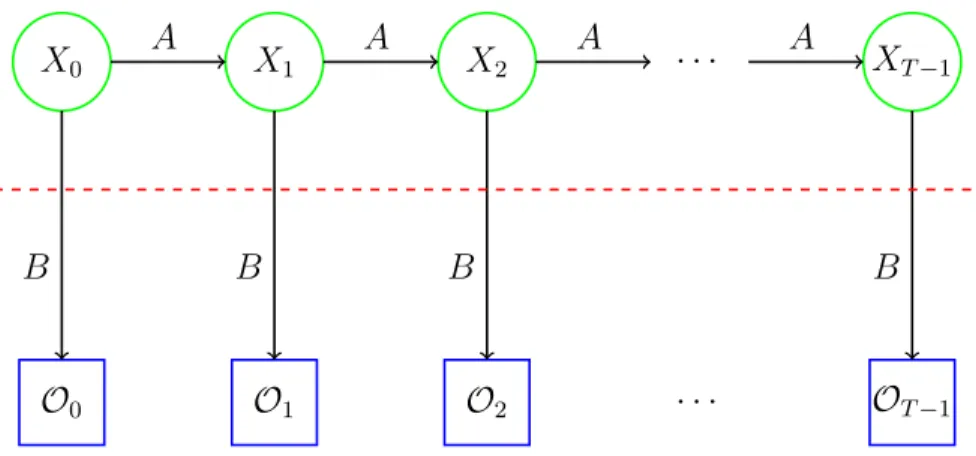
Figure 1 gives a graphical view of the Hidden Markov Process. The state and observation of HMM at any point of time 𝑡 is represented by 𝑋𝑡 and 𝒪𝑡
respectively, as shown in Figure 1.
3.1.2 Implementation
In our implementation we start of by training a Hidden Markov Model based on set of given metamorphic malware files. Once the model has been trained this model represents the statistical properties that define the given
𝒪0 𝒪1 𝒪2 · · · 𝒪𝑇−1
𝑋0 𝑋1 𝑋2 · · · 𝑋𝑇−1
𝐴 𝐴 𝐴 𝐴
𝐵 𝐵 𝐵 𝐵
Figure 1: Hidden Markov Model
a file under consideration and then predict whether it belongs to the same family that the model was trained upon or not. In the training phase we extracted sequence of opcodes from given executable files by disassembling these files into machine level code. The we created an observation sequence out of these opcode sequence by combining all of them into a long string of opcode sequences.
Once we have trained our HMM on this given observation sequence we can then use this resulting model to score a file under consideration, and then predict whether it belongs to the same family or not. We would have two sets of datasets, the test set and the compare set. The test set comprises of the malware family under our consideration and the compare set usually comprises of benign files. Then we compare the scores generated by the files in test set to those generated by files in the compare set. Our main aim here is to get a clear separation between the scores generated by each of these data sets. In terms of LLPO our model should assign a higher LLPO value tot he files that belong the the malware family under consideration and assign a lower score to the comparison data set i.e. the benign files.
After training a HMM on NGVCK virus files we use it to score a subset of NGVCK malware files and also an equivalent number of benign files(Cygwin files). Then we compare the scores generated by the test data set compris-ing of the NGVCK files against those generated by the comparison data set comprising of the benign files.
3.2 Opcode Graph Similarity
The given malware file is first disassembled to generate a sequence of opcodes. This sequence of opcodes is then used to generate a directed graph. To construct this directed graph, first of all we create nodes representing all the unique opcodes that we encounter in the given malware file. Once we have all the edges for this graph we insert edges between each pair of nodes which occur as consecutive opcodes in the given file i.e. a directed edge is constructed for each pair of opcodes opc1 and opc2 such that opc2 follows opc1 in the sequence of opcodes for that particular file. The weight of that edge is defined as the probability of these two opcodes in that particular order.
3.2.1 Implementation
Here our main aim is to construct an opcode graph for each file and then compare opcode graphs from two files to generate a similarity score between those two files. For this we go through the sequence of opcodes in a given file and create an opcode graph. We create a weighted directed graph wherein each node consists of a unique opcode in our file and the edges connecting different opcodes are created for each opcode bigram in that file. We create this graph for both the malware files as well as the benign files. For comparison we can
then use these opcode graphs instead of the actual files. Here we discuss the approach that has been previously studied in the paper [23].
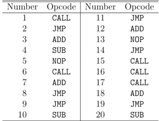
Table 1 shows a subset of assembly language trace from a given metamor-phic file:
Table 1: Opcode Sequence
Number Opcode Number Opcode
1 CALL 11 JMP 2 JMP 12 ADD 3 ADD 13 NOP 4 SUB 14 JMP 5 NOP 15 CALL 6 CALL 16 CALL 7 ADD 17 CALL 8 JMP 18 ADD 9 JMP 19 JMP 10 SUB 20 SUB
Table 2 shows a matrix containing count for each instruction digram in the given file. There is a count value against each row-column opcode pair if they exist in the opcode sequence one after the other and the value is determined as the sum of all such occurences. So, the value against row 1 col 3 corresponds to the count of instruction digrams involving ADD followed by JMP. Then, we convert this table into a row-stochastic table by dividing each count by the number of columns in the table. This leads to a matrix which provides us with transition probabilities between successive opcodes as shown in Table 3. Then, we generate a weighted directed graph for this table as shown in figure 2.
Table 2: Opcode Count
ADD CALL JMP NOP SUB
ADD 0 0 2 1 1
CALL 2 2 1 0 0
JMP 2 1 1 0 2
NOP 0 1 1 0 0
SUB 0 0 1 1 0
Table 3: Probability Table
ADD CALL JMP NOP SUB
ADD 0 0 12 14 14 CALL 25 25 15 0 0 JMP 13 16 16 0 13 NOP 0 12 12 0 0 SUB 0 0 12 12 0 ADD CALL JMP NOP SUB 1/4 1/4 1/2 1/3 1/2 2/5 1/5 1/6 1/2 1/3 2/5 1/6 1/2 1/2
Once we have the graph, we need to establish a threshold value which can then be used to compare different scores by following the below steps:
1. Determine the opcode graphs for a set of malware family. 2. Determine the opcode graphs for a set of benign files.
3. Compute the scores for all pairs of metamorphic family viruses from step 1.
4. Determine the scores for differing pairs comprising of one family malware from step 1 and one benign file from step 2.
5. Establish threshold values based on results from step 3 and step 4.
Once a threshold score has been established, we can use this score to compare different sets of files. Now, to check if a given file belongs to a particular malware family or not, we would first generate an opcode graph for the given file. Then, we can compare this graph with that of a file from the malware family in consideration. Once we have this score we can compare it to our threshold value, if it is greater then the threshold value then we classify the given file as a benign file otherwise as a malware file belonging to the same family.
3.3 Simple Substitution Distance
It is an efficient technique which uses the similarity measure between two given files for detection of metamorphic malware. This technique again relies on the fact that we have a representative set of malware files belonging to the same family. Here, we use a distance measure similar to the method used in
cryptanalysis, which is based on simple substitution distance. This method uses a hill climbing approach based on Jakobsen’s algorithm [13]. The main idea behind the approach is based on the frequency of opcodes, assuming that they stay the same for a given family. So, we can use Jakobsen’s algorithm to compare the similarity of a given file against both a malware file and a benign file.
3.3.1 Jakobsen Algorithm
Jakobsen’s algorithm is an algorithm which involves refining an initial guess for the encryption key with each iteration. It is based on the assumption that the cipher text is actually in English language and has only 26 different symbols. So, each of these symbols represents a letter in the english language. it is a very fast algorithm because the distribution matrix is only created once and is then changed after every iteration to evaluate the plain text.
The algorithm starts of by calculating the frequency of all the symbols in the cipher text. Once all the frequencies have been calculated we can sort them in reverse order. Then we can compare the maximum frequencies from the cipher text to english language character frequencies and generate a putative key. The algorithm then runs various iterations to improve on this key as follows:
3.3.2 Implementation
In our implementation we follow the same approach of extracting opcode sequences from all the family files as discussed in the previous two sections. Then we create bigram distribution matrix from these opcode sequences which
Algorithm 1 Jakobsen’s Fast Attack on substitution ciphers 1: Initialize𝐸 with expected digram frequencies
2: 𝐶 = Input cipher text
3: 𝐾 = Compute Initial Putative Key
4: 𝑃 = Putative plaintext by decrypting C using K 5: 𝐷 = Digram distribution matrix for P
6: 𝑠𝑐𝑜𝑟𝑒 =𝑑(𝐷, 𝐸) 7: for 𝑖= 1 to 𝑛−1 do 8: for 𝑗 = 1 to 𝑛−𝑖 do 9: 𝐷′ =𝐷 10: swapRows(j, j+i) 11: swapColumns(j, j+i)
12: if d(D′,E) < score then
13: 𝐷=𝐷′
14: swapElements(j, j+i) {Swap elements of the putative key}
15: score = d(D’,E)
16: end if
17: end for
18: end for 19: return K
is the equivalent of𝐸 matrix in Jackobsen’s algorithm [13]. Then we construct another similar matrix for the file which we want to classify, this matrix is equivalent of 𝐷 matrix in the algorithm. We constrain both of these matrices to the most common𝑛 opcodes. We add one more symbol to represent all the other opcodes which were excluded from the list. So, we are left with 𝑛+ 1
symbols.
Then we choose an initial “key” 𝐾 such that it is a representative of the frequency of opcodes in the malware family. We assume that the frequencies of opcodes in family viruses should be the same as compared to the code that we are suspecting.
Then we construct the equivalent of matrix 𝐷 by using the key 𝐾 to decrypt. This is similar to the procedure followed in Jackobsen’s algorithm to
construct𝐷. Once we have the𝐸and𝐷matrices we make them row stochastic so that the scores are not dependent on the size of the opcode sequence. For example, if we have the below mentioned opcodes:
MOV,CALL,ADD,XOR,CMP
where the opcodes are in a reverse sorted order of their frequencies. Assume that the sequence that we want to score is:
JMP,MOV,MOV,ADD,INC,INC,INC
the frequency counts for these will be:
Table 4: Opcode Frequency Counts
Opcode INC MOV ADD JMP
Frequency 3 2 1 1
So, our initial guess for the putative key 𝐾 is: Table 5: Initial Putative Key Guess
Metamorphic Family MOV CALL ADD XOR
File to be scored INC MOV ADD JMP
By using the above putative key 𝐾 the decrypted sequence results in:
XOR,CALL,CALL,ADD,MOV,MOV,MOV
This gives us our initial 𝐷 matrix which is also referred to as digraph distri-bution matrix as shown in table 6.
fol-Table 6: Digraph Distribution Matrix
MOV CALL ADD XOR CMP OTHER
MOV 2 0 0 0 0 0 CALL 0 1 1 0 0 0 ADD 1 0 0 0 0 0 XOR 0 1 0 0 0 0 CMP 0 0 0 0 0 0 OTHER 0 0 0 0 0 0
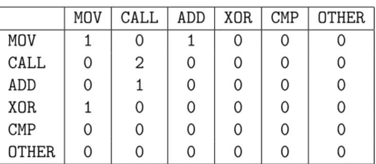
if we are looking at the first row then we will swap MOV and CALL, to achieve this we can just swap the first row with the second row and repeat the same with columns. This will result in our modified matrix shown in table 7.
Table 7: Modified Digraph Distribution Matrix
MOV CALL ADD XOR CMP OTHER
MOV 1 0 1 0 0 0 CALL 0 2 0 0 0 0 ADD 0 1 0 0 0 0 XOR 1 0 0 0 0 0 CMP 0 0 0 0 0 0 OTHER 0 0 0 0 0 0
From here onwards our algorithm carries on in the same way as in Jack-obsen’s algorithm [13]. The score for a given file is computed as the score of the final𝐷 matrix. In our implementation we limit the size of our matrices to 25, based on previous research done in paper [24].
CHAPTER 4 Support Vector Machines 4.1 Introduction
Support vector machines are an example of supervised learning algorithms which belong to both the regression and classification categories of machine learning algorithms. SVMs is a collection of machine learning algorithms that can be used to recognize pattens in given data [5]. Given a set of training data we would like to classify new examples into one of the possible two categories. For achieving such a task SVM training algorithm can be used to build a model which is capable of performing such classification. We can define the SVM model by having all the example from the training data represented as points on a space. These points will be represented in the two dimensional space such that there is an evident gap between data points belonging to our two different classes. So for new points we can use this model to classify it to one of these two classes based on which side of the gap it belongs to. This kind of classification is known as linear classification [28].
4.1.1 SVM Example
SVM’s can be defined by using the concepts of decision planes and support vectors. The decision planes are planes in the two dimensional space that would represent the decision boundaries. Basically a decision plane is defined as a plane which completely separates all data points belonging to two different classes. Figure 3 shows an example of data points in two dimensional space.
Red and Green dots. The Green points refer to class A whereas Red points refer to class B. If we look at the figure we can clearly see that we can plot a line segment which can separate all the data points in a way that all points belonging to one class are on one side and all the other points are on the other side of the line segment. This line segment will be our decision plane. Any new examples of data coming in can be classified based on this line segment, if it falls on the left side then it belongs to class B otherwise it belongs to class A [28].
Figure 3: Linear Classifier
The type of classification shown in Figure 3 is referred to as linear classi-fication, i.e. the classifier separates two different classes of data by finding a decision plane in between them.
But in some cases the classification problem is much tougher then the one shown in Figure 3. An example of a different kind of classification problem is shown in Figure 4. If we compare the two figures we can clearly see that the classification task in the second is tougher and we cannot have a simple line segment separating the two classes. In such situations we would have to plot a curve instead. Classification problems which involve plotting of simple line segments to differentiate between data points belonging to two different kinds
are referred to as hyper plane classifiers [28]. These kind of problems are best suited for Support Vector Machines.
Figure 4: Non Linear Classifier
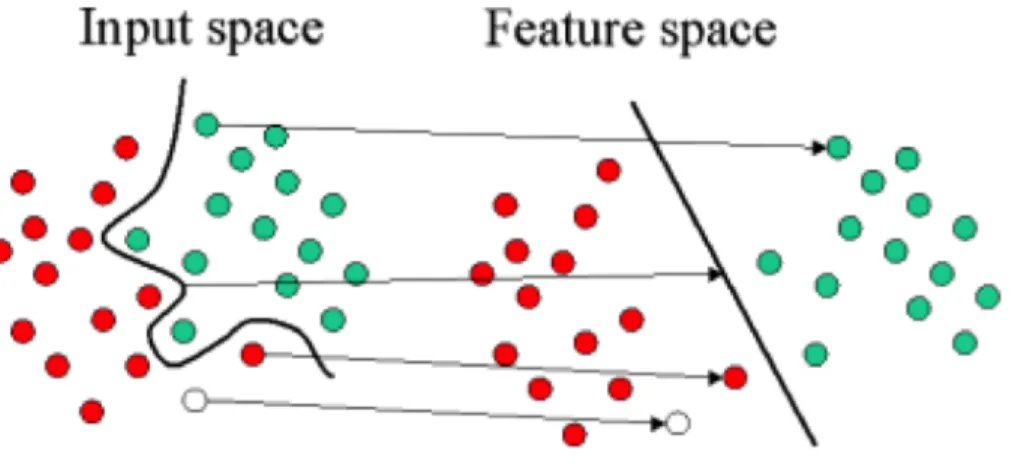
But sometimes there are cases wherein we cannot separate the datasets linearly. In such scenario’s support vector machines allow us to use a special trick known as the kernel trick. A kernel trick is basically using some math-ematical functions which are known as “kernels” to map the given data sets into a new feature space(mapping). The only condition here is that when we map our data points into this new feature space, the newly mapped points should be linearly separable in this new feature space. So, we can change the complex problem of plotting a curve into a simple problem of plotting a line segment in the new feature space. Figure 5.
4.1.2 Kernel Mapping
Definition: A kernel is defined as a function that accepts two vectorsx𝑖
andx𝑗 as inputs and produces an output which is defined as the inner product
Figure 5: Kernel Mapping
We are not concerned about the dimensionality of the newly formed space because we are only returning the inner products in the new space for the two vectors.
The main idea here is to generate a learning algorithm that operates in kernel space, which is generated by substituting the values of all inner products from the original space into the newly formed kernel space:
𝑓(x) = 𝜑(x)𝑇w+𝑏= 𝑚
∑︁
𝑗=1
𝛼𝑗𝑦𝑗𝐾(x,x𝑗) +𝑏
The parameter 𝑏 can be found from any support vectors x𝑖
𝑏=𝑦𝑖 −𝜑(x𝑖)𝑇w=𝑦𝑖− 𝑚 ∑︁ 𝑗=1 𝛼𝑗𝑦𝑗(𝜑(x𝑖)𝑇𝜑(x𝑗)) =𝑦𝑖− 𝑚 ∑︁ 𝑗=1 𝛼𝑗𝑦𝑗𝐾(x𝑖,x𝑗)
4.1.3 Linear separation of a feature space
Let’s assume that we have a hyper plane in an 𝑛-dimensional (𝑛-D) orig-inal feature space
𝑓(x) = x𝑇w+𝑏= 𝑛
∑︁
𝑖=1
where w= [𝑤1,· · ·, 𝑤𝑛]𝑇 the weight vector is normal to the hyper plane,
and|𝑏|/||w||is defined as the distance between the plane and origin [11]. Then we can say that our 𝑛-Dimensional has been partitioned into two different regions by this new hyper plane [11]. We can go ahead and define a mapping function 𝑦=sign(𝑓(x))∈ {1,−1}, i.e.,
𝑓(x) = x𝑇w+𝑏=
{︂
>0, 𝑦 =sign(𝑓(x)) = 1, x∈𝑃 <0, 𝑦 =sign(𝑓(x)) =−1, x∈𝑁
Any point x∈ 𝑃 which exists on the positive side is mapped to 1, while any pointx∈𝑁 which exists on the negative side is mapped to -1. A pointx of unknown class will be classified to 𝑃 if 𝑓(x)>0, or 𝑁 if 𝑓(x)<0[11].
4.1.4 The learning problem
Given a set𝐾 training samples from two linearly separable classes 𝑃 and
𝑁
{(x𝑘, 𝑦𝑘), 𝑘= 1,· · · , 𝐾}
where 𝑦𝑘 ∈ {1,−1} labels x𝑘 to belong to either of the two classes. Our main
aim is to find a hyper-plane in terms of w and 𝑏, that linearly separates the two classes.
Before w is properly trained, the actual output 𝑦′ =sign(𝑓(x)) may not be the same as the desired output 𝑦. There are four possible cases:
Input (x, 𝑦) Output 𝑦′ =sign(𝑓(x)) result
1 (x, 𝑦 = 1) 𝑦′ = 1 =𝑦 corrrect
2 (x, 𝑦 =−1) 𝑦′ = 1̸=𝑦 incorrect
3 (x, 𝑦 = 1) 𝑦′ =−1̸=𝑦 incorrect
The weight vectorwis updated whenever the result is incorrect (mistake driven):
∙ If(x, 𝑦 =−1)but 𝑦′ = 1̸=𝑦 (case 2 above), then xnew =wold+𝜂𝑦x=wold−𝜂x When the samex is presented again, we have
𝑓(x) = x𝑇wnew+𝑏 =x𝑇wold−𝜂x𝑇x+𝑏 <x𝑇wold+𝑏
The output 𝑦′ =sign(𝑓(x))is more likely to be 𝑦=−1as desired. Here
0< 𝜂 <1 is the learning rate.
∙ If(x, 𝑦 = 1) but 𝑦′ =−1̸=𝑦 (case 3 above), then wnew=wold+𝜂𝑦x=wold+𝜂x When the samex is presented again, we have
𝑓(x) = x𝑇wnew+𝑏=x𝑇wold+𝜂x𝑇x+𝑏 > x𝑇wold+𝑏
The output 𝑦′ =sign(𝑓(x))is more likely to be 𝑦 = 1 as desired.
Summarizing the two cases, we get the learning law:
if 𝑦𝑓(x) =𝑦(x𝑇wold+𝑏)<0, then wnew =wold+𝜂𝑦x The two correct cases (cases 1 and 4) can also be summarized as
𝑦𝑓(x) = 𝑦(x𝑇w+𝑏)≥0
4.1.5 Definition
For a decision hyper-plane x𝑇w+𝑏 = 0 to separate the two classes P (x𝑖,1) and N (x𝑖,−1), it has to satisfy
𝑦𝑖(x𝑇𝑖 w+𝑏)≥0
for bothx𝑖 ∈𝑃 andx𝑖 ∈𝑁. Among all the planes that can actually satisfy our
condition, we are concerned in finding a plane that can separate the given two classes in such a way that the margin between them is the maximum possible margin [11].
The optimal plane which maximizes the margin has to lie somewhere in between the two classes, to make the distance from the closest points on each of its sides equal. We then draw two more planes 𝐻+ and𝐻− that are parallel
to each other and also to 𝐻0 and also pass through the closest point to the plain on both of its sides:
x𝑇w+𝑏 = 1, and x𝑇w+𝑏 =−1
All points x𝑖 ∈𝑃 on the positive side should satisfy x𝑇𝑖 w+𝑏≥1, 𝑦𝑖 = 1
and all points x𝑖 ∈𝑁 on the negative side should satisfy x𝑇𝑖 w+𝑏≤ −1, 𝑦𝑖 =−1
These can be combined into one inequality
The equality holds for those points on the planes 𝐻+ or 𝐻−. Such points are
called support vectors, for which
x𝑇𝑖 w+𝑏 =𝑦𝑖
i.e., the following holds for all support vectors
𝑏=𝑦𝑖−x𝑇𝑖 w=𝑦𝑖− 𝑚 ∑︁ 𝑗=1 𝛼𝑗𝑦𝑗(x𝑇𝑖 x𝑗) 4.2 Implementation
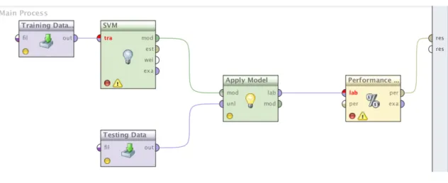
In our implementation of the SVM’s we used Rapid-miner studio a tool available with multiple machine learning packages. This learner uses the Java implementation of the support vector machine mySVM by Stefan Rueping. The implementation of mySVM can both be utilized in regression task as well as classification tasks and it provides a very fast implementation which gives good results. mySVM works with all kind of functions, be it linear or quadratic and it is also useful in case of asymmetric loss functions [27]. Figure 6 below shows the design of the SVM process.
4.2.1 Design
Training Data: This corresponds to the training input file which is expected to be an excel file with labelled data in form of tuples defined above.
Testing Data: This corresponds to the testing input file which is ex-pected to be an excel file with un-labelled data in form of tuples defined above.
SVM: This is the learner which generates a model by learning from the Training data.
Figure 6: SVM Design
Apply Model: This operator allows us to apply a model onto incoming testing data.
Performance: This operator provides us with a list of performance cir-teria’s which can be used to measure its performance and also for visualization purposes.
4.2.2 Algorithm
Figure 7 explains the scoring process in detail. In our scenario we are us-ing the SVM as a classifier which can classify Benign and Metamorphic files. The features that our SVM is built on correspond to the scores that we re-ceived from HMM, Simple Substitution and Opcode graph scoring techniques as discussed in previous sections. The algorithm works in two phases -Training Phase and Testing Phase. In Training Phase, we generate a model by training on our training dataset which is formed by combining the scores from our three different techniques i.e. HMM, Simple Substitution and Opcode graph as a tuple along with a class description referring to as either Benign or Metamor-phic file as shown in Figure 7. In Testing Phase, we apply the model that we
created in the training phase to our testing dataset which is again the same tuple along with a class description as shown in Figure 7.
CHAPTER 5 Experiments
In this chapter we focus our attention on using the below mentioned tech-niques to score a representative set of metamorphic malware:
∙ Hidden Markov Model Method
∙ Opcode Graph Similarity Method
∙ Simple Substitution Distance Method
∙ Combining all the above three using SVM’s
The first three of these methods work directly on the statistical properties of opcodes and the last method works by combining the scores coming out of these three techniques. Our test set of metamorphic viruses consists of 200 NGVKC files [31]. So all the results to follow in this chapter will revolve around the NGVCK family to be representative of metamorphic files [25]. The NGVCK family of viruses in previous researches has proved that it is one of the most highly metamorphic [33].
Our set of benign files consists of 40 cygwin utility files [6]. We have se-lected these files for our experiments because we wanted to compare our results with previous implementations which also used these files in their experiments, including [33]. Finally we will be diversifying our malware dataset by moving to a whole new families of metamorphic malware in the next chapter. We use
ROC (Receiver Operating Characteristics) curves for comparing these tech-niques to each other and for measuring their efficacy [4]. The Area under the curve also refer to as AUC in coming sections, which is the area under this ROC curve will provide us with a measure of the degree of correctness of each of these techniques.
We used a machine with the below mentioned configuration: Table 8: Machine Specification
Model MacBook Pro Retina
Processor 2.4 GHz Intel Core i5
RAM 8 GB 1600 MHz DDR3
System type 64-bit OS
Operating System OS X 10.9.5
5.1 Receiver Operating Characteristics
Receiver Operating Characteristics or in short ROC curve is a kind of graph which is drawn to measure the correctness of a binary classifier [4]. We first calculate the TPR also known as true positive rate which is defined as the number of positives that were predicted positives in actual out of the total predicted positives. Then we calculate FPR also known as false positive rate which is defined as the negative classifications which were accidentally predicted as positives out of the total actual negatives. Once we have these two values we plot the TPR vs the FPR at different levels of threshold to generate an ROC curve. TPR is also known as sensitivity and FPR is also known as the fall out of a classification system [9].
In the following sections we will be discussing about the results of the above mentioned techniques in detail. We will be plotting ROC curves to
compare their efficiency. We will also be using area under the curve or in short AUC for these ROC curves as a measure of the correctness of these scoring systems.
5.2 Hidden Markov Model Method
We did a lot of experiments so as to compare the results that we got for our implementation against the scores produced in previous researches [23]. While performing our experiments we saw that the final score produced is not effected much by the number of states that we have considered for the HMM. So, we decided to go with 2 as the default number of states for HMM in our experiments. In this particular experiment, we trained our HMM on a training set which consisted of 160 NGVCK files to generate a model which we could use for scoring similar files. Then we used this model to score another testing set which consisted of 40 NGVCK files alongwith a compare set consisting of 40 Benign files. If we look at the scatter plot in Figure 8 we can clearly see that there is a clear separation between the scores for both kind of files.
Figure 9 shows the corresponding ROC curve that has been plotted for the results received in this experiment. From the curve it is very easy to deduce that our HMM model is capable of producing great results and can easily distinguish the family viruses from benign files. The AUC for this experiment was 1.0, which further reinstates the fact that it produces perfect classification.
Figure 8: HMM Score Analysis
5.3 Opcode Graph Similarity
This experiment is based around the same setup where we use a subset of 160 NGVCK files for the training phase and use the remaining 40 files along with 40 cygwin utility files for the testing dataset. We use the process defined in Section 3.2.1 to establish a threshold value, which will further be used for the actual distinction between the two type of files.
Figure 10 shows a scatterplot that we got after plotting the results from our experiment. The red dots in the scatter plot denote the similarity score between two different types of files in our experiment i.e. the malware and benign files, whereas blue triangles denote the similarity score between two files which belong to same malware family. Because there is a clear separation between the two scores in Figure 10, we can clearly conclude that this method is able to distinguish between the files correctly.
Figure 10: Opcode Graph Similarity Score Analysis
the results received in this experiment. From the curve it is very easy to deduce that our Opcode graph similarity method is capable of producing great results and can easily distinguish the family viruses from benign files. The AUC for this experiment was 1.0, which further reinstates the fact that it produces perfect classification.
Figure 11: ROC curve for Opcode Graph Similarity Method
5.4 Simple Substitution Distance
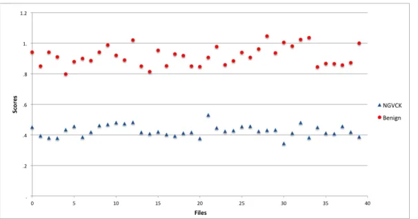
In this experiment as well we used the same malware and benign files as discussed above. The scores obtained in this experiment are plotted on scatter plot as shown in Figure 12. From the scatter plot it is quite clear that the malware files produce a lower score for this technique as compared to the benign files which are quite different.
Figure 12: Simple Substitution Method Score Analysis
the results received in this experiment. From the curve it is very easy to deduce that our Simple Substitution method is capable of producing great results and can easily distinguish the family viruses from benign files. The AUC for this experiment was 1.0, which further reinstates the fact that it produces perfect classification.
5.5 Support Vector Machine
In this experiment we are not devising a new technique for detection of metamorphic malware by working on any of its characteristics, rather our aim here is to see if we could combine the scores coming from the three techniques defined above and use an SVM classifier to classify them. So, here rather than directly working with malware and benign files we will be working with scores generated by the three previous techniques as described in Section 5.2, 5.3, 5.4. Once we have scores from the above three techniques, we split them into two files with each containing a tuple:
Figure 13: ROC curve for Simple Substitution Method
(𝑎𝑐𝑡𝑢𝑎𝑙 𝑐𝑙𝑎𝑠𝑠 𝑙𝑎𝑏𝑒𝑙, 𝐻𝑀 𝑀 𝑠𝑐𝑜𝑟𝑒, 𝑂𝐺𝑆 𝑠𝑐𝑜𝑟𝑒, 𝑆𝑆𝐷 𝑠𝑐𝑜𝑟𝑒)
The output from the support vector machine is a file which contains a tuple:
(𝑎𝑐𝑡𝑢𝑎𝑙 𝑐𝑙𝑎𝑠𝑠 𝑙𝑎𝑏𝑒𝑙, 𝐻𝑀 𝑀 𝑠𝑐𝑜𝑟𝑒, 𝑂𝐺𝑆 𝑠𝑐𝑜𝑟𝑒, 𝑆𝑆𝐷 𝑠𝑐𝑜𝑟𝑒, 𝑝𝑟𝑒𝑑𝑖𝑐𝑡𝑒𝑑 𝑐𝑙𝑎𝑠𝑠 𝑙𝑎𝑏𝑒𝑙)
as shown in Figure 7. We can then compare the predicted class label against the actual class for calculating the performance of the model. The scores obtained in this experiment are plotted on scatter plot as shown in Figure 14. It can be observed that our SVM technique is able to distinguish between metamorphic malware and benign file with an accuracy of 100%.
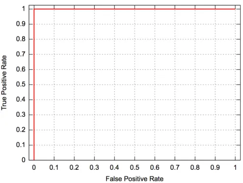
Figure 15 shows the corresponding ROC curve that has been plotted for the results received in this experiment. From the curve it is very easy to deduce that our Support vector machine method is also capable of producing results that are similar to the one’s produced by the underlying techniques. The AUC for this experiment was 1.0, which shows that it can easily distinguish
Figure 14: Support Vector Machine Score Analysis the metamorphic family files from benign files.
Figure 15: ROC curve for Support Vector Machine Method
Model, Simple Substitution Distance and Opcode Graph Similarity techniques. In the coming sections we will do an in-depth analysis of the robustness of our underlying techniques that we have discussed above.
CHAPTER 6 Results
In the previous section we have seen that Support Vector Machines can be used to detect malware files from benign files by using scores from different techniques. In the coming sections we will test the robustness of each of these techniques. Our main aim is to prove that Support Vector Machines can serve as a more robust detection strategy even when the underlying techniques have failed.
6.1 Attacks on Detection Techniques
In this section, we consider the robustness of the above mentioned meta-morphic detection techniques. In previous researches [15] for attacks on these statistical metamorphic detection techniques, it has been observed that mor-phing the metamorphic malware files by inserting code from benign files gives the best results.
6.1.1 Morphing Techniques
In [15], a morphing engine was developed in order to evade detection by known machine learning techniques such as the Hidden Markov Model technique. The engine works by inserting dead code from a benign file into a metamorphic file so as to beat the statistics of the metamorphic file which make it susceptible to detection by HMM [23].
pa-∙ Block Morphing
∙ Random Morphing
In the first case, which we refer to as “block morphing”, the dead code is inserted as a single block of code which is placed into the malware file at one location. Whereas in “random morphing”, the dead code is inserted uniformly into the malware file at constant intervals so as to spread the dead code throughout its body. The paper proves that this method of insertion of “dead code” into the malware file from a benign file is capable of defeating the HMM detection, i.e. it is able to induce false negatives or false positives. In the paper it has also been shown that the first method of insertion that is block morphing is way more effective then the random morphing method.
We performed experiments at different levels of block morphing. The amount of dead code inserted into the file depends on the size of the malware file and is usually inserted as a percentage of its size. For example in order to do a 20% morphing into a metamorphic file of 400 lines we would have to insert 80 lines into it from a randomly selected benign file. The main point to be noted here is that all the steps we are performing here are happening at the assembly code level, but we are just making these changes to the static opcode files that we already have. The assumption here is that in real world a malware writer would have to put in a lot of effort to do the same modifications into an executable, because he has to make sure that none of the inserted code gets executed. Another thing that he has to worry about is that the inserted code should not look obvious and should not be easily detected by someone debugging the executable. So, by ignoring these practical problems which are
involved in the insertion of dead code into a malware file, we are considering the worst possible case that a malware writer would have to go through. In the coming sections we look at results of our detection techniques against block morphed NGVCK malware files.
6.2 Results for Morphed Malware 6.2.1 Hidden Markov Model Method
We started off by inserting different levels of opcodes into the NGVCK files from randomly selected benign files. In Figure 16, we show a scatter plot for HMM results for 10% morphed NGCVK malware files vs Benign files, from the scatter plot it is clearly visible that there is no clear distinction between the malware scores and the benign scores at 10% block morphing.
Figure 16: HMM - 10% morphed Scores Analysis
The ROC curve shown in Figure 17 below validates the fact, it can be clearly inferred from the ROC curve that some of the files have been
miss-value of 1.000 for un-morphed Malware files vs Benign Files.
Figure 17: HMM - ROC curve for 10% morphing
Table 9 shows AUC value for ROC Curves plotted for different levels of block morphing. From the table we can see that there is a considerable drop in the AUC values at 10% and 20% block morphing levels, but the AUC values for morphing levels greater than 20% tend to stabilize. Figure 18 shows the graph for these results.
Table 9: HMM AUC values for different levels of Block Morphing
Morphing percentage AUC
0% 1.00000
10% 0.90125
20% 0.81625
30% 0.81875
Figure 18: HMM AUC at different Morphing levels(Table 9)
6.2.2 Opcode Graph Similarity Method
In this experiment we inserted different percentages of opcodes into the NGVCK files from randomly selected benign files. In Figure 19 we show a scatter plot for Opcode Graph Similarity method results for 60% morphed NGCVK malware files vs Benign files, from the scatter plot is clearly visible that there is no clear distinction between the malware scores and the benign scores at 10% block morphing. This technique turned out to be comparatively more robust to HMM technique as it could withstand morphing levels of upto 50% before showing any kind of miss-classification.
The ROC curve shown in Figure 20 below validates the fact, it can be clearly seen from the ROC curve that some of the files have been miss-classified at 60% block morphing level. The AUC for Figure 20 has been reduced to
Figure 19: OGS - 60% morphed Scores Analysis
0.91250 from its initial value of 1.000 for un-morphed Malware files vs Benign Files.
Figure 20: OGS - ROC curve for 60% morphing
of block morphing. From the table we can see that Opcode graph similarity technique is more robust than HMM technique as at relatively moderate levels of morphing it produced perfect results in the form of AUC value of 1.0. It was only at about 60% block morphing the the results started to deteriorate and the AUC value dropped to 0.91250. Figure 21 shows the graph for these results.
Table 10: OGS AUC values for different levels of Block Morphing
Morphing percentage AUC
0% 1.00000 10% 1.00000 20% 1.00000 30% 1.00000 40% 1.00000 50% 1.00000 60% 0.91250
6.2.3 Simple Substitution Distance Method
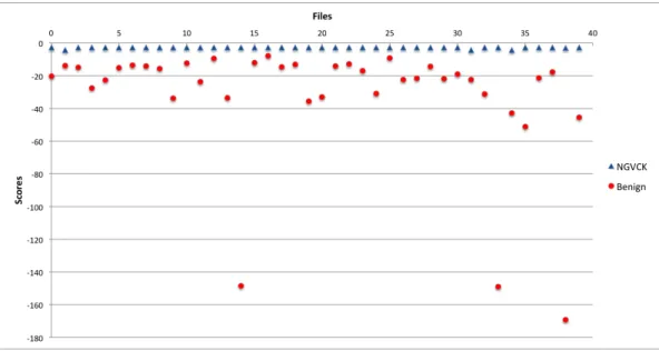
In this experiment as well we inserted different percentages of opcodes into the NGVCK files from randomly selected benign files. In Figure 22 we show a scatter plot for Simple Substitution Distance method scores for 80% morphed NGCVK malware files vs Benign files, from the scatter plot it is clearly visible that there is no clear distinction between the malware scores and the benign scores at 80% block morphing. This technique turned out to be comparatively more robust to HMM technique, because it could withstand morphing levels of upto 50% before showing any kind of miss-classification. It performed a little better in comparison to the Opcode Graph Similarity technique as well, it took about 80% block morphing to drop the AUC value to 0.89875 whereas similar AUC was achieved in case of Opcode Graph Similarity at a morphing level of 60%.
Figure 22: SS - 80% morphed Scores Analysis
clearly seen from the ROC curve that some of the files have been miss-classified at 80% block morphing level. The AUC for Figure 27 has been reduced to 0.89875 from its initial value of 1.000 for un-morphed Malware files vs Benign Files.
Figure 23: SS - ROC curve for 80% morphing
Table 11 shows AUC values for ROC curves plotted for different levels of block morphing. From the table we can see that Opcode graph similarity technique is more robust than HMM technique as at relatively moderate levels of morphing it produced perfect results in the form of AUC value of 1.0. It was only at about 60% block morphing that the results started to deteriorate and the AUC value dropped to 0.91250. Figure 24 shows the graph for these results.
Table 11: SS AUC values for different levels of Block Morphing
Morphing percentage AUC
0% 1.00000 10% 1.00000 20% 1.00000 30% 1.00000 50% 1.00000 60% 0.99750 70% 0.95063 80% 0.89875
Figure 24: SSD AUC at different Morphing levels(Table 11)
6.2.4 Combining Scores using SVM
In this experiment we want to see if SVM can provide us with better result than individual scores from the three techniques mentioned above. Because the maximum morphing % used to break all the techniques was registered in case of Simple Substitution method, wherein it took about 80% block morphing to bring the AUC down by a considerable level, we choose 80% morphing as a benchmark. Now we generate scores for each of the three techniques at 80% block morphing. Figure 25, 26, 27 below show the ROC curves generated by each of the three techniques at 80% block morphing.
Figure 25: HMM - ROC curve for 80% morphing
Figure 26: OGS - ROC curve for 80% morphing
In comparison to these above three, we can see that Support vector ma-chine can produce better results by combining the scores from the above three techniques. Figure 28 shows the ROC curve generated by SVM scores. The AUC for this ROC curve is 1.0, which is better than the AUC achieved by any
Figure 27: SS - ROC curve for 80% morphing
We summarize these results in Table 12. If we take a look at the table it is evident that SVM produced a perfect AUC score of 1.0 when all the individual techniques had failed with AUC scores around 0.9. So we can conclude that SVM’s can produce better results by combining scores generated by different malware detection techniques. Figure 29 shows the graph for these results.
Table 12: Comparison of Scores at 80% Block Morphing
Scoring Technique AUC
Hidden Markov Models 0.85062
Opcode Graph Similarity 0.89875
Simple Substitution Distance 0.88437
Support Vector Machine 1.00000
6.2.4.1 SVM Kernel functions comparison
We tested different kernel methods for our SVM implementation, but got the best results with radial kernel as shown in Table 13. So from here on, all our experiments will be using the radial function as the kernel function.
Figure 28: SVM - ROC curve for 80% morphed scores
Table 13: Comparison of SVM Kernel Functions at 80% Block Morphing SVM Kernel AUC Dot 0.918 Polynomial 0.860 Neural 0.850 Radial 1.000 6.3 SVM vs Individual Techniques
In this section we compare the results produced by SVM against the re-sults produced by each of our individual techniques. In Section 6.2.4 we saw that SVM scores outperformed each of the techniques at a morphing level of 80%. Next we try to establish a morphing ratio wherein SVM’s perform better than each of the individual techniques. Table 14 shows AUC values at differ-ent morphing percdiffer-entages for Hidden Markov Model(HMM), Opcode Graph Similarity(OGS), Simple Substitution Distance(SSD) and Support Vector Ma-chine(SVM) techniques respectively. From the table we can see that SVM is a much more robust technique as compared to the other three.
Table 14: Comparison of Scores at Different Morphing levels
Morphing % HMM AUC OGS AUC SSD AUC SVM AUC
0% 1 1 1 1 10% 0.90125 1 1 1 20% 0.81625 1 1 1 30% 0.81875 1 1 1 40% 0.82250 1 1 1 50% 0.86250 1 1 1 60% 0.87875 0.91250 0.99750 1 70% 0.85437 0.90687 0.95063 1 80% 0.85062 0.88437 0.89875 1 90% 0.87625 0.87250 0.93812 1 100% 0.90000 0.85370 0.90750 1 110% 0.9 0.79563 0.90188 0.97906 120% 0.9 0.78125 0.87438 0.95875
Figure 30 shows a line graph depicting the change in AUC values at different morphing levels for all the four techniques. We can clearly see that SVM performs way better than the other techniques even at 100% morphing level. The morphing ratio where SVM shows up to be better than the three underlying techniques is 60%. Now that we have proved that SVM’s can be used to combine results from different malware detection techniques and still produce better results, we would like to put it to test against some other virus families to see how it performs as compared to the three underlying techniques.
Figure 30: Comparison of AUC Values at different Morphing levels
6.3.1 ZeroAccess Malware
In this experiment we want to validate how SVM performs against the in-dividual techniques for ZeroAccess Malware. We extract the opcode sequences from the ZeroAccess malware files and use them as the dataset for our malware