Clustering versus SVM for Malware Detection

San Jose State University

SJSU ScholarWorks

Master's Projects Master's Theses and Graduate Research

Spring 5-25-2015

Clustering versus SVM for Malware Detection

Usha Narra

San Jose State University

Follow this and additional works at:https://scholarworks.sjsu.edu/etd_projects

Part of theArtificial Intelligence and Robotics Commons, and theInformation Security Commons

This Master's Project is brought to you for free and open access by the Master's Theses and Graduate Research at SJSU ScholarWorks. It has been accepted for inclusion in Master's Projects by an authorized administrator of SJSU ScholarWorks. For more information, please contact

[email protected].

Recommended Citation

Narra, Usha, "Clustering versus SVM for Malware Detection" (2015).Master's Projects. 405. DOI: https://doi.org/10.31979/etd.sgwj-a5ab

Clustering versus SVM for Malware Detection

A Project Presented to

The Faculty of the Department of Computer Science San Jose State University

In Partial Fulfillment

of the Requirements for the Degree Master of Science

by Usha Narra

c

○2015 Usha Narra

The Designated Project Committee Approves the Project Titled

Clustering versus SVM for Malware Detection

by Usha Narra

APPROVED FOR THE DEPARTMENTS OF COMPUTER SCIENCE

SAN JOSE STATE UNIVERSITY

May 2015

Mark Stamp Department of Computer Science Robert Chun Department of Computer Science Fabio Di Troia Università del Sannio

ABSTRACT

Clustering versus SVM for Malware Detection by Usha Narra

Previous work has shown that we can effectively cluster certain classes of mal-ware into their respective families. In this research, we extend this previous work to the problem of developing an automated malware detection system. We first compute clusters for a collection of malware families. Then we analyze the effectiveness of clas-sifying new samples based on these existing clusters. We compare results obtained using 𝑘-means and Expectation Maximization (EM) clustering to those obtained us-ing Support Vector Machines (SVM). Usus-ing clusterus-ing, we are able to detect some malware families with an accuracy comparable to that of SVMs. One advantage of the clustering approach is that there is no need to retrain for new malware families.

ACKNOWLEDGMENTS

I would like to express my gratitude to my project advisor, Dr. Mark Stamp for his continued support and guidance throughout the project. He has always been very patient in explaining things and very encouraging through out the project.

A very special thanks to my committee member, Fabio Di Troia for his valuable inputs and suggestions.

I would also like to thank my committee member, Dr.Robert Chun for his time and guidance.

Last but not least, I would like to thank my husband, Mr.Jayachandra Gullapalli for his support and guidance throughout my Masters.

TABLE OF CONTENTS

CHAPTER

1 Introduction . . . 1

2 Malware Detection and Concealment Strategies . . . 4

2.1 Malware . . . 4 2.1.1 Virus . . . 4 2.1.2 Worm . . . 5 2.1.3 Trojan Horse . . . 5 2.1.4 Spyware . . . 5 2.2 Detection Techniques . . . 6 2.2.1 Signature Detection . . . 6 2.2.2 Change Detection . . . 7 2.2.3 Anomaly Detection . . . 7 2.2.4 HMM Based Detection . . . 8 2.3 Concealment Strategies . . . 13 2.3.1 Encrypted Virus . . . 14 2.3.2 Polymorphic Virus . . . 14 2.3.3 Metamorphic Virus . . . 15 3 Related Work . . . 16 3.1 MEDiC . . . 16

3.2 Behavior Based Malware Detection . . . 18

3.4 HMM for Malware Classification . . . 20

4 Clustering and SVM . . . 22

4.1 Clustering . . . 22

4.1.1 Clustering Techniques . . . 22

4.1.2 Expectation Maximization (EM) Clustering . . . 23

4.1.3 Cluster Validation . . . 25

4.2 Support Vector Machines (SVM) . . . 28

5 Implementation and Experimental Setup . . . 30

5.1 Dataset . . . 30

5.2 Training the HMMs . . . 31

5.2.1 Training with compilers and malware generators . . . 32

5.2.2 Training with subset of malware samples . . . 33

5.3 Clustering Implementation . . . 33

5.3.1 Clustering scores from compiler trained HMM models . . . 34

5.3.2 Clustering scores from malware trained HMM models . . . 35

5.4 SVM Implementation . . . 37

5.5 Experimental Setup . . . 37

6 Results . . . 39

6.1 Clustering . . . 39

6.1.1 Clustering results of compiler trained HMM scores . . . 39

6.1.2 Clustering results of malware trained HMM scores . . . 40

6.1.3 Comparison of clustering algorithms based on accuracy . . 46

6.2.1 SVM results of compiler trained HMM scores . . . 50 6.2.2 SVM results of malware trained HMM scores . . . 51

7 Conclusion and Future Work . . . 56

LIST OF TABLES

1 HMM Notation . . . 9

2 Dataset Distribution . . . 31

3 Number of files used for training HMMs . . . 32

4 Distribution of Samples Used for Clustering . . . 35

5 Probability Scores of EM and𝑘-means . . . 41

6 AUC for different kernel functions (7-tuple data) . . . 51

7 AUC for different kernel functions (2-D data) . . . 52

8 AUC for different kernel functions (3-D data) . . . 53

9 AUC for different kernel functions (4-D data) . . . 54

LIST OF FIGURES

1 Generic View of HMM . . . 9

2 Silhouette Coefficient Example . . . 27

3 Optimal Hyperplane Example . . . 28

4 Transformation of Data to Higher Dimensional Space . . . 29

5 Probability Score Comparison . . . 40

6 ROC curve for EM clustering algorithm (2-D data) . . . 41

7 Cluster formation using EM clustering algorithm (2-D data) . . . 42

8 ROC curve for 𝑘-means clustering algorithm (2-D data) . . . 43

9 Cluster formation using𝑘-means clustering algorithm (2-D data) 43 10 ROC curve for EM clustering algorithm (3-D data) . . . 44

11 ROC curve for 𝑘-means clustering algorithm (3-D data) . . . 45

12 ROC curve for EM clustering algorithm (4-D data) . . . 45

13 ROC curve for 𝑘-means clustering algorithm (4-D data) . . . 46

14 Accuracy measure for EM algorithm . . . 48

15 Accuracy measure for𝑘-means algorithm . . . 48

16 Accuracy comparison of EM and 𝑘-means algorithms . . . 49

17 ROC curve for SVM algorithm (7-tuple data) . . . 50

18 ROC curve for SVM algorithm (2-D data) . . . 51

19 ROC curve for SVM algorithm (3-D data) . . . 52

CHAPTER 1 Introduction

Malware is a piece of software that runs unauthorized tasks without the consent of the user. The tasks performed by malware intend to do harm to the user by gaining access to their sensitive information stored on the system or by tricking the user to provide their personal and/or financial information. To protect the user, system and any critical information stored on it, malware has to be identified and eliminated from the system. Malware is a broad term that encompasses various types of computer viruses, worms, trojan horses, spyware, adware etc. A more detailed view on different kinds of malware is presented in Chapter 2.

Stuxnet is an advanced form of malware (worm) that is known worldwide for its attack on industrial control systems. The distinguishing feature that makes Stuxnet stand out from other worms is its access control over physical systems [45]. Stuxnet came to light in the year 2010, June. It was programmed to infect the industrial programmable logic controllers (PLC’s), targeting Iran’s nuclear facilities. Stuxnet exploits vulnerabilities in industrial control systems and spreads through removable USB drives. A component of Stuxnet (rootkit) hid all the background activity on the system.

Koobface is a type of malware that is platform independent and spreads through social networking sites. It wouldn’t be an exaggeration to say that every person who has access to internet uses social networking sites these days. Koobface takes advantage of this fact and targets the users on social networking sites such as Skype, Facebook, Twitter and mailing services like GMail and Yahoo Mail! Koobface is not a

single module of code, it contains several units each performing its respective task. All the units coordinate with each other to form the Koobface worm. The worm resides in the spam of these websites and the users who encounters it get infected. From the infected system, the Koobface collects the user’s login details and also other user profile information from any social networking sites accessed from that system. One important unit that works to the advantage of Koobface is its rouge DNS (Domain Name System) changer unit which prevents the user form accessing anti-virus software or security websites [44].

It is clear from the above information that malware is a serious threat in this digital era. According to [43], malware or harmful programs are adapting to the increasing use of anti-virus software at a fast rate and are growing more powerful, posing danger to the community at large. Some malware stay dormant for a long time and are capable of spreading rapidly across the network when they encounter loopholes in the security of the system. Anti-virus software is the most widely used defense mechanism against malware, but are not capable of detecting advanced malware. Most anti-virus software use signature based detection which identifies a malware by its signature. The drawback of this technique is it cannot identify obfuscated or new class of malware that does not match the list of known signatures. By the time security experts identify the new malware and trace out its signature, the malware would have enough time to carryout its actions. There are several other techniques used to detect malware which are discussed in Chapter 2. Inspite of all the existing techniques, there is no classification model that can differentiate the new malware and fit it into the existing models. More research and experiments are needed in the area of detection of malware to develop a technique which can effectively combat evolving malware.

In this paper, we apply Hidden Markov Models (HMM) and clustering techniques to the problem of classifying new/unknown malware. The combination of HMM and clustering techniques is inspired from previous research in malware classification [2, 3]. The basic idea of this paper is to train the HMMs [47] for different malware fami-lies. These trained models are then used to score malware samples. Based on these scores, the malware samples are grouped into clusters using Expectation Maximiza-tion (EM) [9] and𝑘-means clustering algorithms [1]. Analysis of the resulting clusters indicate that HMM-based clustering can be an effective tool for classifying new/pre-viously unknown malware. We compare the results of both the clustering techniques to see which one does a better job in classifying different malware families. We also classify the same malware samples using Support Vector Machines (SVM) to see how well clustering performs as compared to SVM.

This paper is organized as follows: Chapter 2 defines various kinds of malware and describes some of the existing malware detection techniques and concealment strategies adopted by malware writers. Chapter 3 provides insight into previous work done on malware classification. Chapter 4 provides details about Clustering (espe-cially EM clustering) and SVM, while Chapter 5 discusses our implementation and experimental setup for clustering and SVM in more detail. In Chapter 6 experimental results are presented and analyzed. Finally, Chapter 7 contains our conclusion and suggestions for future work.

CHAPTER 2

Malware Detection and Concealment Strategies

2.1 Malware

Malware is a computer program that performs malicious actions [46]. Unlike a bad piece of software which may not provide the intended functionality due to accidental bugs in the code, malware is written to cause harm.

As mentioned in Chapter 1, malware is used to refer computer infections such as worms, viruses, spyware, trojan horses, adware etc. A short description of the various types of malware is as follows:

2.1.1 Virus

Majority of the known malware today are viruses. A computer virus is a self-replicating program that links itself to other executables to spread the infection. This implies that the infected program is capable of spreading the infection to the other executable programs [21]. Virus may conceal itself anywhere in the system such as the executable files, data files, hidden folders or even in the boot sector. A virus that resides in the boot-sector of the hard drive is known as boot-sector virus and it becomes active at the start-up of the system [7]. Thus it makes itself immune to any anti-virus software that starts with the booting of the system or even before any security at the operating system level is enabled. As it is one of the first programs to run during the boot process, it can even block anti-virus software from executing on the system. Some of the historic examples of computer viruses are Brain, Lehigh, MBDF, Pathogen, Melissa [34].

2.1.2 Worm

Worms are similar to the viruses as they create copies of themselves except that worms do not require a host file. Thus they differ from viruses which require an infected host file for spreading [40]. According to [4], worms are independent programs and they do not depend on other host files. A worm usually spreads on a network compromising the systems on its way in the network. Some of the examples of famous worms are Morris, Ramen, Lion, Adore, Code Red, Nimda [30].

2.1.3 Trojan Horse

A Trojan horse is a malware which pretends to do some legitimate task, but secretly performs malicious tasks [4]. Trojan horse differs from virus as it does not spread itself [40]. They camouflage as harmless programs or files that the end users might mistake for authentic programs and use them [37]. But when the user runs the programs assuming them to be known software, the trojans perform undesired activities in the background. Some of the notable trojan horses are Netbus, Subseven, Back Orifice [30].

2.1.4 Spyware

Spyware is a form of malware when installed in a system steals the user’s creden-tials from the system of which the user is unaware of [25]. Spyware generally conceals itself and collects data related to keystrokes, browsing patterns, credit card details, personal information etc. At times the activities of the spyware can get far beyond normal monitoring and carries out activities such as installing additional software, reducing connection speeds, redirecting web browser searches, changing computer settings etc [25]. Unlike viruses and worms, spyware do not usually make copies of

themselves. Some of the examples of spyware are CoolWebSearch, HuntBar, Weath-erStudio, Zango, Zlob [23].

2.2 Detection Techniques

Most anti-virus software in use today depend on static detection techniques. Static analysis extracts interesting features from file without executing the file and studies them whereas dynamic analysis extracts the actual behavior of the file by running it in a sandbox. In this section we look at some of the static malware detection techniques, for example, signature detection, change detection, anomaly detection and HMM based detection.

2.2.1 Signature Detection

Amongst static detection techniques, signature detection is the most popular one. Signature detection depends on discovering a series of bits (signature) which uniquely identifies a particular malware [31]. That is, the anti-virus scanner scans all the files in the system looking for some specific signatures. The anti-virus software saves all the signatures of known malware in a database and frequently updates this database to include any new signatures. When the scanner finds a match within the list of known malware signatures in its database, the file will be marked as malware. Signature detection works on known malware whose signature is already in the database. The major disadvantage of this approach is it cannot detect new (previously unknown) or even obfuscated malware. Also, another important factor to consider in signature detection is the signature database. The efficiency of this technique entirely depends on the quality of the database. To have an effective detection rate, the database must be regularly updated [31].

2.2.2 Change Detection

When a file is infected by malware, the contents of the file are changed. Change detection monitors the files looking for any unapproved changes [4]. The basic idea behind this technique is to calculate the hash values of all the files on the system and save them in a file. From time to time we re-calculate the hashes of all files and compare them with the actual hash values saved in the file. Any mismatch in hash values indicates that the file has been modified, which indicates that the file might have be infected with malware. That is, change detection checks the integrity of the files on the system periodically and reports red flags.

One advantage with change detection is that any changes to a file can be detected without fail which guarantees that this technique could atleast detect if not classify new malware. But the real problem with change detection is that files on a system change regularly and this may prompt numerous false positives thereby reducing the efficiency of detection [31].

2.2.3 Anomaly Detection

Anomaly-based detection is based on the organization of file contents [13]. The structural details of a file can be considered as its attributes. These attributes are extracted and provided to a machine learning algorithm that is trained to classify ordinary from anomalous file structures. But there is no set definition for normal and unusual structure of programs. This poses a fundamental challenge to anomaly detection, defining what is normal and what is unusual. Depending on how we train the learning model and the definitions we give for normal and unusual behavior, there may be numerous false positives and false negatives.

a malware detector model which can classify the files on the system into different categories based on the structural organization of the files. Any new file that needs to be categorized is given to the detector model. If the file looks similar to the model, it is marked as benign otherwise as malware. When a file is marked as malware it is further reviewed to determine whether it is actually malicious or just a false positive. Since anomaly detection alone might give numerous false positives, it is often combined with other techniques such as signature-based detection for further screen-ing [31].

2.2.4 HMM Based Detection

Some of the previous research [2, 47] prove that HMM can be an effective tool for malware detection. Apart from malware detection, HMMs are also used for speech recognition [27], gene prediction, human activity recognition [26], etc. In the following sections we give a brief overview of HMM and how it is used for malware detection.

2.2.4.1 Introduction to HMM

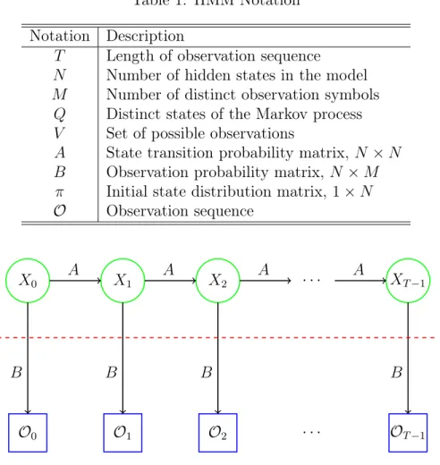
In general, a Markov process is a statistical model in which the internal states and state transitions are transparent to the user. A HMM can be considered as a special case of Markov model as the states in HMM are not visible to the user (hid-den), consequently the name ‘Hidden’ Markov Model. Table 1 provides the standard notation used for HMM.

The three matrices𝐴, 𝐵and𝜋together represent the HMM. These three matrices are row stochastic in nature. A matrix is said to be row stochastic if the sum of all the elements in a row is equal to 1. So, an HMM can be written in terms of these matrices as 𝜆= (𝐴, 𝐵, 𝜋). Figure 1 illustrates a generic view of Hidden Markov Model.

Table 1: HMM Notation Notation Description

𝑇 Length of observation sequence

𝑁 Number of hidden states in the model

𝑀 Number of distinct observation symbols

𝑄 Distinct states of the Markov process

𝑉 Set of possible observations

𝐴 State transition probability matrix, 𝑁 ×𝑁 𝐵 Observation probability matrix, 𝑁 ×𝑀

𝜋 Initial state distribution matrix, 1×𝑁

𝒪 Observation sequence

𝒪0 𝒪1 𝒪2 · · · 𝒪𝑇−1

𝑋0 𝑋1 𝑋2 · · · 𝑋𝑇−1

𝐴 𝐴 𝐴 𝐴

𝐵 𝐵 𝐵 𝐵

Figure 1: Generic View of HMM

We can solve three problems using HMM. The three problems and algorithms to solve these problems [32] are as follows:

Problem 1:

Given a model 𝜆 = (𝐴, 𝐵, 𝜋) and an observation sequence 𝒪, we want to find the probability 𝑃(𝒪|𝜆).

Problem 2:

Given a model 𝜆 = (𝐴, 𝐵, 𝜋) and an observation sequence 𝒪, we want to find the most likely hidden state sequence of the model.

Problem 3:

Given a scenario where the observation sequence 𝒪 and dimensions 𝑁 and 𝑀

are known, the model 𝜆 which increases the probability of 𝒪 need to be found. For the research presented in this paper, HMM models are trained to represent different compilers and malware families. This is similar to problem 3 mentioned above. A large collection of malware and benign samples are scored using these HMM models. Again, this is similar to problem 1 mentioned above. So, in this paper we are going to use the HMM algorithms that solve the Problems 1 and 3. Now, we discuss these HMM algorithms (forward algorithm, backward algorithm and Baum-Welch algorithm) to solve these problems in detail.

Solution to Problem 1:

Our aim in problem 1 is to find the probability of an observation sequence,

𝑃(𝒪|𝜆) with respect to 𝜆 = (𝐴, 𝐵, 𝜋). To find the 𝑃(𝒪|𝜆) we use the forward algorithm or𝛼-pass. For𝑡= 0,1, . . . , 𝑇 −1 and 𝑖= 0,1, . . . , 𝑁 −1, we define

𝛼𝑡(𝑖) = 𝑃(𝒪0,𝒪1, . . . ,𝒪𝑡, 𝑥𝑡=𝑞𝑖|𝜆). (1) where 𝛼𝑡(𝑖) corresponds to the probability of the partial observation sequence until time 𝑡, when the Markov process is in state 𝑞𝑖 at time𝑡.

The forward algorithm can be computed recursively as follows:

1. Let 𝛼0(𝑖) = 𝜋𝑖𝑏𝑖(𝒪0), for 𝑖= 0,1, . . . , 𝑁 −1

2. For 𝑡 = 1,2, . . . , 𝑇 −1and 𝑖= 0,1, . . . , 𝑁 −1, compute

𝛼𝑡(𝑖) = [︂𝑁−1 ∑︁ 𝑗=0 𝛼𝑡−1(𝑗)𝑎𝑗𝑖 ]︂ 𝑏𝑖(𝒪𝑡)

3. From Equation (1), the desired probability is given by 𝑃(𝒪|𝜆) = 𝑁−1 ∑︁ 𝑖=0 𝛼𝑇−1(𝑖) Solution to Problem 2:

Our aim in problem 2 is to find the most likely state sequence. In order to do that, we use the backward algorithm or 𝛽-pass. This is similar to the forward algorithm, except as the name suggests it starts at the end and finds its way to the beginning. For 𝑡= 0,1, . . . , 𝑇 −1 and 𝑖= 0,1, . . . , 𝑁 −1, we define

𝛽𝑡(𝑖) =𝑃(𝒪𝑡+1,𝒪𝑡+2, . . . ,𝒪𝑇−1|𝑥𝑡=𝑞𝑖, 𝜆). The backward algorithm can be computed recursively as follows:

1. Let 𝛽𝑇−1(𝑖) = 1, for 𝑖= 0,1, . . . , 𝑁 −1

2. For 𝑡 =𝑇 −2, 𝑇 −3, . . . ,0 and 𝑖= 0,1, . . . , 𝑁 −1, compute

𝛽𝑡(𝑖) = 𝑁−1

∑︁

𝑗=0

𝑎𝑖𝑗𝑏𝑗(𝒪𝑡+1)𝛽𝑡+1(𝑗)

For𝑡 = 0,1, . . . , 𝑇 −2and 𝑖= 0,1, . . . , 𝑁 −1we define,

𝛾𝑡(𝑖) = 𝑃(𝑥𝑡 =𝑞𝑖|𝒪, 𝜆),

Since 𝛼𝑡(𝑖) measures the relevant probability until time 𝑡 and 𝛽𝑡(𝑖) measures the probability after time𝑡, we can write𝛾𝑡(𝑖)as follows

𝛾𝑡(𝑖) =

𝛼𝑡(𝑖)𝛽𝑡(𝑖)

𝑃(𝒪|𝜆) (2) Solution to Problem 3:

Our aim in problem 3 is to train a model that best fits the observations. One of the interesting aspects of HMM is its ability to re-estimate the model itself. We already know the size of the matrices 𝐴, 𝐵 and 𝜋, we just need to find the elements of these matrices. In order to find these elements, we use the Baum-Welch algorithm. Initially we define “di-gammas” as,

𝛾𝑡(𝑖, 𝑗) = 𝑃(𝑥𝑡 =𝑞𝑖, 𝑥𝑡+1=𝑞𝑗|𝒪, 𝜆) for 𝑡= 0,1, . . . , 𝑇 −2 and 𝑖= 0,1, . . . , 𝑁 −1.

Where 𝛾𝑡(𝑖, 𝑗)is the probability of being in state 𝑞𝑖 at time𝑡 and going to state

𝑞𝑗 at time 𝑡+ 1. Writing the di-gammas in terms of 𝛼, 𝛽, 𝐴 and 𝐵 gives,

𝛾𝑡(𝑖, 𝑗) =

𝛼𝑡(𝑖)𝑎𝑖𝑗𝑏𝑗(𝒪𝑡+1)𝛽𝑡+1(𝑗)

𝑃(𝒪|𝜆) (3)

Equations (2) and (3) are related as follows:

𝛾𝑡(𝑖) = 𝑁−1

∑︁

𝑗=0

𝛾𝑡(𝑖, 𝑗)

Re-estimating the model is an iterative process. The process starts by initializing the model, 𝜆= (𝐴, 𝐵, 𝜋) with random values such that 𝜋𝑖 ≈1/𝑁 and 𝑎𝑖𝑗 ≈1/𝑁 and

𝑏𝑗(𝑘)≈1/𝑀.Note that the values of 𝐴, 𝐵, 𝜋 are random. This is important to note because if we initialize the matrices with exactly uniform values, the model might get stuck in a local maximum. The iterative process can be summarized as follows:

1. Initialize, 𝜆 = (𝐴, 𝐵, 𝜋).

2. Compute 𝛼𝑡(𝑖), 𝛽𝑡(𝑖), 𝛾𝑡(𝑖, 𝑗) and 𝛾𝑡(𝑖).

For𝑖= 0,1, . . . , 𝑁 −1, let

𝜋𝑖 =𝛾0(𝑖)

For𝑖= 0,1, . . . , 𝑁 −1and 𝑗 = 0,1, . . . , 𝑁 −1,compute

𝑎𝑖𝑗 = 𝑇−2 ∑︁ 𝑡=0 𝛾𝑡(𝑖, 𝑗) ⧸︂𝑇−2 ∑︁ 𝑡=0 𝛾𝑡(𝑖) For𝑗 = 0,1, . . . , 𝑁 −1and 𝑘= 0,1, . . . , 𝑀 −1, compute

𝑏𝑗(𝑘) = ∑︁ 𝑡𝜖(0,1,...,𝑇−2),𝒪𝑡=𝑘 𝛾𝑡(𝑗) ⧸︂𝑇−2 ∑︁ 𝑡=0 𝛾𝑡(𝑗) 4. If 𝑃(𝒪|𝜆) increases, go to 2.

2.2.4.2 HMM for Malware Detection

A trained HMM model can be used to classify malware from benign samples. There is a lot of previous work done on using HMM for malware detection. According to [47], we can ‘train’ an HMM on a set of files such that the trained model represents a particular family (either malware or benign on which it has been trained). Now, given a new observation sequence which is not a part of training data, we can score the sequence using the trained HMM. The model will output a high score if the sequence is similar to the training data and output a low score otherwise. In an ideal case, the model should output a score of 1 for a sequence on which it has been trained.

Previous research [2, 15] has shown that HMMs trained on opcode sequences and/or function call-graphs can effectively classify different families of malware.

2.3 Concealment Strategies

With more and more malware detection software coming into light, malware writers are using many concealment strategies to prevent their malware from being

detected by regular malware detection techniques. Some of the concealment strategies are discussed below:

2.3.1 Encrypted Virus

As mentioned in Section 2.2.1, signature detection is the most commonly used malware detection technique. One basic approach used even by novice malware writ-ers to evade signature detection is encryption [5]. The major advantage of encrypted virus is it does not need strong cryptographic encryption techniques. A simple en-cryption such as XOR operation on the malware file completely changes the signature of the malware. But the set back is an encrypted virus cannot execute directly be-cause the instructions are encrypted and cannot be read by the system. In order to execute the malware, it first needs to be decrypted. So encrypted virus comes as a package containing decryption code and actual encrypted malicious code known as the virus body [28]. So when the malware is executed, the decryption code executes the virus body by decrypting it and provides control to the virus body. The virus now performs its malicious activity.

Encryption seems to be an easy technique to avoid signature detection. But this simple technique comes with a drawback. Instead of trying to find the signature of the virus body, signature detection system can try to find the signature of decryption code which if found could indicate the presence of malware.

2.3.2 Polymorphic Virus

Polymorphic virus is an improvement over encrypted virus. It is built on the same idea as encrypted virus but with additional features to overcome the drawbacks of encryption. The new feature in polymorphic virus is its ability to create a new

decryption code with every infection [28]. As a result, the decryption code looks different across different infections of the same virus. So a single signature of the decryption code cannot detect different generations of the same virus. Even though polymorphic virus can evade signature detection, it can be caught when run in an emulated environment [5].

2.3.3 Metamorphic Virus

Metamorphic virus is built on top of polymorphic malware. Instead of just chang-ing the decryption code with every infection, metamorphic virus changes entire virus body still keeping the virus functionality unchanged. Peter Szor quoted in [41], the shortest definition of metamorphic virus defined by Igor Muttik is “Metamorphics are body-polymorphics”. Every single conceivable strategy appropriate for polymorphic virus to create new decryptor can be utilized by a metamorphic virus to create a new virus body to make another copy of virus [28]. As a result, different generations of metamorphic virus look completely different yet have the same malicious intent.

CHAPTER 3 Related Work

Automatic malware classification is a challenging task and a lot of previous work has been done in this area. Some of the previous research techniques include behav-ioral analysis, compression based analysis etc. One of the recent research papers [2] which inspired the current paper uses clustering techniques to detect malware. In this chapter we discuss some of the previous work done which includes both static and dynamic detection techniques.

3.1 MEDiC

Malware Examiner using Disassembled Code (MEDiC) is a static malware de-tection technique. The underlying logic for MEDiC is an extension of signature-based malware detection. Instead of using the standard signature database, MEDiC cre-ates its own database by extracting necessary features from assembly code. This technique is developed with the intent of detecting obfuscated and mutated malware which cannot be identified by regular signature detection [35]. As the name suggests, the first step in MEDiC is to disassemble the executable file using a disassembler. A disassembler converts machine code into assembly instructions. MEDiC then ex-tracts appropriate subroutines from the assembly code. A subroutine in assembly code consists of a label and instructions associated with it. Since there will be many labels in the assembly code, each subroutine is treated as a checkpoint. Each label and instruction set combination is stored as key-value pairs where label is the key and instructions associated with that label is the value. These key-value pairs are analogous to the signature database. Based on the average length of the subroutine, a

dictionary threshold is determined. This whole process can be considered as building the MEDiC model.

In order to test the MEDiC model, the test file is first disassembled to get the assembly code. Then, the assembly code is parsed to extract the sequence of key-value pairs. The length of each key-value pair is compared with the dictionary threshold value. If the length exceeds the threshold, the key-value pair is counted towards the number of matches and the number of subroutines count towards the number of checks. This process is called MEDiC signature matching. Based on the result of signature matching, the detection algorithm calculates the virus threshold. The virus threshold is calculated as,

virus threshold= number of matches

number of checks

The test file undergoes multiple levels of scanning before it is classified as malicious or benign. The main reason behind multiple scanning is to reduce the number of false positives. In the first level of scanning, the checkpoints extracted from the test file are matched against the signature database. If more checkpoints match the signature database than the virus threshold the file is marked as malicious. If the file passes this level, it enters second level of scanning where the key names are excluded in the matching process. This second level of scanning is trying to match similar instruction sets with different labels. In the third level the raw assembly code instructions are matched against the signature database. We can observe that with each level, the scanning becomes more generalized. Since MEDiC uses disassembled code, the authors in [35] claim that this model can detect malware on any operating system.

3.2 Behavior Based Malware Detection

Behavior-based malware detection as the name suggests extracts the dynamic behavior of the files and studies this behavior to detect malware. Dynamic behavior of a file can be extracted by executing the file in an emulated (sandbox) environment. The emulated environment allows the user to see step by step execution of the pro-gram. Many emulators provide a convenient user interface where the user can specify which characteristics of the file to identify and report. The research methodology in [11] combines the features extracted from dynamic analysis with machine learning (classification) techniques for effective and efficient malware detection.

As with all the malware detection techniques, this technique also has training and testing phases. In the training phase, data samples (both malware and benign) are collected and monitored for behavioral patterns. This is done by passing each file through an automatic dynamic analysis tool which executes the file in an emu-lated environment. As mentioned above, the emulator generates a behavioral report of the input file. These report files are preprocessed for feature selection. Feature selection is the process of selecting only the crucial and applicable characteristics for further processing. These selected features from each file are stored as vectors. Ma-chine learning techniques are applied on these vector models for further learning and classification. The research in [11] compares five different machine learning classifiers namely𝑘-Nearest Neighbor, Naïve Bayes, Support Vector Machine, J48 decision tree and Multilayer Perceptron (MLP) neural network of which J48 gives better perfor-mance results.

3.3 Compression Based Malware Detection

Several machine learning techniques are in use for the purpose of identifying un-known malware. Since machine learning techniques are supervised algorithms, they require labeled and organized input data. Despite the fact that machine learning techniques provide promising results, the limiting factor with these techniques is the requirement of labeled input. However the raw data from the executable files is not structured. So we cannot directly apply machine learning algorithms on raw executable files. The data from the files must be preprocessed and converted into desirable format for the algorithm. Preprocessing generally involves feature selection and extraction, labelling the extracted features, etc. Such preprocessing might intro-duce errors into the data and may not use all the available data for learning. The research methodology in [48] proposes a new malware detection technique that does not require any preprocessing, thereby working on raw executables.

Compression is the process of reducing the size of a file. This is achieved by re-moving redundancy in a file. The basic logic behind compression is to assign a unique symbol to each string and replace all the occurrences of the string with its correspond-ing symbol thereby reduccorrespond-ing the size of the file considerably. The research in [48] uses an adaptive data compression model namely prediction by partial matching (PPM). The detection mechanism in this paper [48] builds two compression models using the PPM algorithm. One of the compression models represent malware class and the other represents benign class. Each file that needs to be classified, is encoded (compressed) using the two compression models. Whichever model yields the best compression output in terms of compression ratio determines the classification of the file. The preliminary results shown in [48] are promising.

3.4 HMM for Malware Classification

The current research is inspired from the work in [2]. As discussed in Chapter 2, HMM can be used for malware detection. The research in [2] combines HMM and

𝑘-means clustering to come up with a malware classification model to classify over 8000 malware samples. Initially several HMM models are trained on a variety of compilers and malware generators (GCC, MinGW, TurboC, Clang, TASM, NGVCK and MWOR). Each malware file is scored against all the trained HMM models. As a result, each of the malware sample is represented by a 7-tuple score. These 7-tuple scores are provided to the 𝑘-means clustering algorithm.

In 𝑘-means clustering, a dataset of 𝑛 samples is partitioned into 𝑘 clusters such that each data point belongs to one and only one cluster which has the nearest centroid. The 𝑘-means algorithm involves the following steps:

1. Specify the number of clusters 𝑘.

2. Choose initial centroids. The initial centroid estimate can be chosen either at random or uniformly across the dataset.

3. We then associate each data point to the nearest centroid (squared euclidean distance measure is used to compute the distance from each data point to all the centroids).

4. Re-compute the cluster centroids based on current clustering of data points. 5. If there is a significant change in centroids, re-associate the data points to the

nearest centroid.

Once the samples are clustered, Receiver Operating Characteristics (ROC) curves are plotted to find the accuracy of cluster formations. The clustering algorithm is performed for varied values of 𝑘 (from 2 to 15) and the results in [2] show that by using 𝑘-means clustering on HMM scores, the malware samples can be classified into clusters of appropriate families with good accuracy. But the major drawback of 𝑘 -means algorithm is that the algorithm does not consider the underlying distribution of the data and the cluster formations depend heavily on the initial choice of the centroids.

To overcome this drawback of 𝑘-means algorithm, we use EM clustering in this project. More details about EM algorithm are given in the next chapter.

CHAPTER 4 Clustering and SVM

4.1 Clustering

Clustering is the process of grouping objects together such that related objects fall in same group. Clustering is a common technique used in statistical data anal-ysis, data mining, pattern recognition, etc. This section will briefly discuss various categories of clustering algorithms and then look at EM clustering in detail.

4.1.1 Clustering Techniques

∙ Intrinsic vs Extrinsic: Intrinsic clustering is an unsupervised learning method and hence is directly applied to the data. In unsupervised learning, we do not have class labels for the data [33]. On the other hand, extrinsic clustering is a supervised learning method. In supervised learning, prior to running the algorithm, data is preprocessed to assign class labels such that each data point belongs to one of the classification classes [33].

∙ Agglomerative vs Divisive: In agglomerative clustering each data point is con-sidered a cluster in itself [33]. As the algorithm proceeds, the nearest data points merge together forming fewer large clusters. This process continues until all the clusters are merged into a single cluster. Since the algorithm starts with multiple small clusters and works its way up to a single large cluster, it is known as “bottom-up” approach. In contrast, divisive clustering starts with a single cluster consisting of all data points [42] and as the algorithm proceeds, the large cluster is split into multiple mini sized clusters. Hence, divisive clustering can be viewed as a “top-down” approach [33].

∙ Hierarchical vs Partitional: Hierarchical clustering is in a way related to divi-sive clustering except for the hierarchical relationship. That is in hierarchical clustering, when a large cluster is split into few small clusters, the large and the small clusters are bound by a parent-child relation respectively. The hierarchi-cal relationship between the clusters can be pictorially represented in the form of a dendrogram [33]. On the other hand, clusters in partitional algorithm do not share any relationship. That is, the data is divided into mutually exclusive clusters such that each data point precisely belongs to one cluster [42].

4.1.2 Expectation Maximization (EM) Clustering

EM clustering is an unsupervised clustering technique. This technique uses gaus-sian mixture models to find the maximum likelihood estimates of the parameters in the data. Unlike𝑘-means clustering, which uses distance measures to classify the data points into different clusters, EM clustering uses existing probability distributions of the data. That is, instead of assigning a data point exclusively to a single cluster, EM clustering calculates the probability with which a data point belongs to each cluster. The data points are then assigned to the cluster with highest probability. Thus, EM clustering can be viewed as soft clustering technique. As the name suggests, the EM algorithm has two steps, namely E-step and M-step. The algorithm iterates between these two steps to find the maximum likelihood of the parameters of the data [6, 33]. The algorithm continues until the parameters converge or the maximum number of iterations is reached. The steps of the EM algorithm are as follows:

∙ Initialize the parameters 𝜃 and 𝜏, where

𝜃𝑖 denotes relevant parameters of distribution 𝑖

∙ E-Step: Using Bayes’ formula, compute the probability of a data point belong-ing to a particular cluster

𝑝𝑗,𝑖=𝜏𝑗𝑓(𝑥𝑖, 𝜃𝑗) ⧸︂ 𝐾 ∑︁ 𝑗=1 𝜏𝑗𝑓(𝑥𝑖, 𝜃𝑗) Where, 𝑗 = 1,2, . . . , 𝐾 (number of clusters)

𝑖= 1,2, . . . , 𝑛 (number of data points)

𝑓 is the probability density function

𝑝𝑗,𝑖 is the probability of 𝑥𝑖 under distribution𝑗

We know that the sum of probabilities of a data point belonging to all the clusters is 1. This is mathematically represented as,

𝐾 ∑︁

𝑗=1

𝑝𝑗,𝑖= 1, (4) for a particular𝑖.

∙ M-Step: Re-estimate the parameters 𝜃 and 𝜏

𝜏𝑗 = 𝑛 ∑︁ 𝑖=1 𝑝𝑗,𝑖 ⧸︂ 𝐾 ∑︁ 𝑗=1 𝑛 ∑︁ 𝑖=1 𝑝𝑗,𝑖 By using (4), the above equation can be simplified as

𝜏𝑗 = 1 𝑛 𝑛 ∑︁ 𝑖=1 𝑝𝑗,𝑖

The estimates for means and variances are given as follows:

𝜇𝑗 = 𝑛 ∑︁ 𝑖=1 𝑝𝑗,𝑖𝑥𝑖 ⧸︂ 𝑛 ∑︁ 𝑖=1 𝑝𝑗,𝑖 𝜎_𝑗2 = 𝑛 ∑︁ 𝑖=1 𝑝𝑗,𝑖(𝑥𝑖−𝜇𝑗)2 ⧸︂ 𝑛 ∑︁ 𝑖=1 𝑝𝑗,𝑖

The parameters 𝜃𝑗 will be some function of𝜇𝑗 and 𝜎𝑗 depending on the proba-bility distribution function.

∙ Iterate between the E-step and M-step until the parameters 𝜃 and 𝜏 converge.

Once the model is converged, each data point is assigned to a cluster for which it has the highest probability. This results in each data point belonging to one cluster. Or, we could allow for soft assignment, where each data point belongs to multiple clusters with relative probability. More implementation specific details of EM clustering are given in chapter 5.

4.1.3 Cluster Validation

Different clustering algorithms can form different clusters with the same data. To compare different clustering algorithms or to quantify how well a particular algo-rithm clusters the data, we should be able to measure individual cluster quality. In this section we will discuss some measures of cluster quality. There are two general approaches to cluster validation, namely, external and internal. We discuss these two approaches in detail in the coming sections.

Let𝑥1, 𝑥2, . . . , 𝑥𝑚 denote the data points and𝐶1, 𝐶2, . . . , 𝐶𝐾 denote the clusters. Let 𝑚𝑗 be the total count of objects in cluster 𝐶𝑗 and 𝑚𝑖𝑗 the number of objects of type 𝑖 in cluster 𝐶𝑗. The probability of having type 𝑖 objects in cluster 𝑗 is given by 𝑝𝑖𝑗 = 𝑚𝑖𝑗/𝑚𝑗. We follow the same notation to discuss the validation techniques below.

4.1.3.1 External Validation

External validation uses metadata about the data to determine the cluster qual-ity. This metadata often corresponds to class labels attached to the data. There are two common measures in external validation, entropy and purity. Both these measures determine the quality of a cluster by counting the number of objects of a particular class assigned to a cluster.

Entropy is a standard measure of instability [14, 33, 42]. Higher entropy implies that the cluster is a mix of objects from multiple classes and no particular class objects dominate the cluster. Following the notation mentioned earlier, entropy of a cluster

𝐶𝑗 is given by 𝐸𝑗 =− 𝑛 ∑︁ 𝑖=1 𝑝𝑖𝑗𝑙𝑜𝑔𝑝𝑖𝑗 The (weighted) intra-cluster entropy is given by

𝐸 = 1 𝑚 𝐾 ∑︁ 𝑖=1 𝑚𝑗𝐸𝑗

We would want 𝐸 to be smaller, since small 𝐸 indicates maximum objects of the cluster belong to a single class.

Purity is the measure of uniformity within the cluster [14, 33, 42]. An ideal cluster should have all the data points of a particular type. Using the same notation as above, purity of a cluster 𝐶𝑗 is defined as

𝑈𝑗 =𝑚𝑎𝑥𝑖𝑃𝑖𝑗 The overall (weighted) purity is given by

𝑈 = 1 𝑚 𝐾 ∑︁ 𝑖=1 𝑚𝑗𝑈𝑗

We would want 𝑈 to be as close to 1 as possible because, smaller 𝑈 indicates that the clusters elements share no relationship with each other.

4.1.3.2 Internal Validation

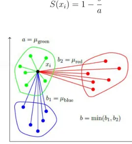
Internal validation determines quality based on cluster characteristics. Naturally, we want the clusters to be well separated from each other. Also, the data points with in a cluster should be as close as possible to each other. These properties are referred to as separation and cohesion respectively. These two properties can be consolidated to get a solitary quality measure called silhouette coefficient [14, 33, 42]. Using the same notation as above, silhouette coefficient of a data point 𝑥𝑖 is given by

𝑆(𝑥𝑖) =

𝑏−𝑎

max(𝑎, 𝑏)

Where,

𝑎 is the average distance of 𝑥𝑖 to the data points in its cluster

𝑏 is the minimum (average distance of 𝑥𝑖 to data points in another cluster) Figure 2 illustrates an example of silhouette coefficient calculation. In general for any reasonable cluster formation, 𝑏 > 𝑎, therefore

𝑆(𝑥𝑖) = 1−

𝑏 𝑎

We would want𝑆(𝑥𝑖)≈1i.e., we want 𝑥𝑖 to be cohesive with respect to the data points in its own cluster and well separated from the data points in other clusters.

In this project we combine purity and silhouette coefficient measures to come up with a score which we use to plot the ROC curves. Implementation details of this score are provided in Chapter 5.

4.2 Support Vector Machines (SVM)

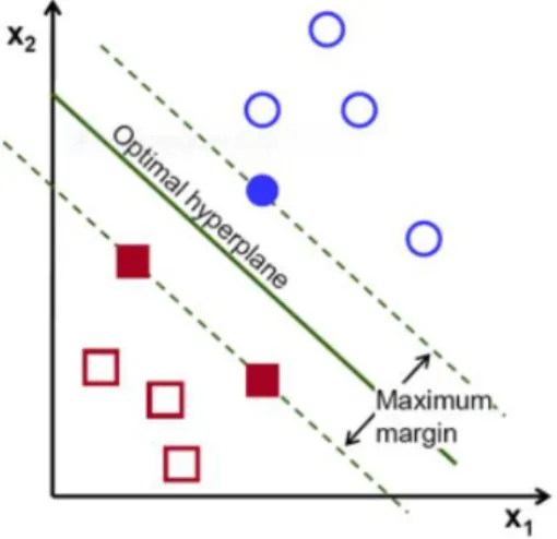
Support Vector Machines are amongst the most popular supervised learning al-gorithms used for classification and regression analysis. Supervised learning method deals with labeled data i.e., we must preprocess the data and assign labels to each data point. SVMs are generally applied to binary classification problems. Given a labeled training data, the algorithm tries to find an optimal hyperplane such that all the data points on one side of hyperplane belong to one class and the data points on other side belong to another class. In other words the hyperplane acts a threshold separating the two classes of data [36]. Figure 3 illustrates an optimal hyperplane separating the red squares from blue circles [24].

The hyperplane should be chosen in such a way that it maximizes the distance between closest data points between the two classes. In other words the hyperplane should maximize the margin as shown in Figure 3. But for most of the real world applications, training data is not linearly separable. There are two ways to deal with this situation. Instead of maximum margin, specify a “soft” margin or use the “kernel trick”. By using soft margin, we allow the SVM to make some classification errors. Depending on the non linearity of the data and the soft margin, the number of classification errors may vary significantly. Kernel trick provides an effective solution to both the problems, non linearity and classification errors.

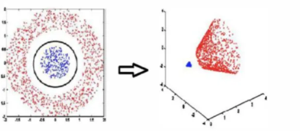
Kernel trick is the process of transforming non linearly separable data into lin-early separable data. This is done by shifting the data into a higher dimensional space [33]. Generally, when dealing with machine learning algorithms, it is advised to reduce the dimensionality of the data so as to avoid the ‘curse of dimensional-ity’. However the kernel trick does the magic in SVM to work efficiently with high dimensional data. The kernel function spreads out the data in high dimensional space making it linearly separable by a high dimensional (one dimension less than the data) hyperplane. Figure 4 illustrates the kernel trick of transforming 2D data into 3D space [19]. Implementation details of SVM are provided in Chapter 5.

CHAPTER 5

Implementation and Experimental Setup

This section provides the implementation and experimental setup details of the project. The first section gives a brief overview of the dataset. The second section gives details about training the HMMs and scoring the dataset. The third section explains the tools and packages used for clustering and the scoring technique used to plot the ROC curves. The fourth section explains the tools used for SVM. Finally, experimental setup details are discussed.

5.1 Dataset

The malware dataset used for this project is obtained from the Malicia project website [22]. The dataset consists of more than 11,000 malware binaries. All the mal-ware files are either an executable (.exe) or a dynamic-link library (.dll). Along with the malware samples, the dataset also consisted of MySQL database with metadata. For each malware sample, the metadata has information of the family of malware and details about when and where the malware is collected. This metadata infor-mation helped us in calculating the cluster purity. Of the 11,000 malware samples, about 7800 samples were distributed among three dominant malware families namely Winwebsec, Zbot and ZeroAccess.

Winwebsec is a malware program that runs only on windows operating system. This malware convinces windows users into buying fake anti-virus software. As an initial step, the malware gives false alerts to the user that the system has been infected even though the system does not contain any other malware. As a commercial step, the malware offers to remove theses infections for a fee [18].

Zbot, also known as Zeus is a family of trojans [38]. Zbot is also targeted to run on windows operating system. This malware steals personal and financial information from the compromised system. Zbot files are usually installed via spam emails and hacked websites [17].

ZeroAccess is another family of trojans that uses advance rootkit to hide itself. ZeroAccess is also targeted at windows users and its major functionality is to download other harmful malware [39].

In this project we only used the malware samples from these three families. The benign samples used for this project are 32-bit Cygwin utility files. Table 2 shows the number of samples used from each family.

All of the malware and benign files are disassembled using the IDA disassem-bler [12]. Opcode sequences are then extracted from the disassembled files and given as input to the HMM models for scoring.

Table 2: Dataset Distribution Family Number of files

Winwebsec 4361

Zbot 2136

ZeroAccess 1306

Benign 213

5.2 Training the HMMs

In this project we perform multiple experiments . All the experiments follow the same steps except that the HMM models are generated with different data. In all the experiments, the HMMs are trained on sequence of opcodes. In order to get the opcodes, the malware and benign binaries are first disassembled using the IDA

disassembler [12]. Opcodes are then extracted from the corresponding assembly files and used to train the HMMs. Now we will see in detail how to train the HMMs for our experiments.

5.2.1 Training with compilers and malware generators

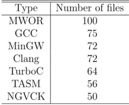
Initially, the HMMs are generated for four different compilers (GCC, MinGW, TurboC, Clang), hand-written assembly (TASM), virus generation kit(NGVCK) and metamorphic malware (MWOR). For each of these models, the training is done for 800 iterations with number of hidden states being 2. The number of assembly files used for training each model is given in Table 3.

Table 3: Number of files used for training HMMs Type Number of files

MWOR 100 GCC 75 MinGW 72 Clang 72 TurboC 64 TASM 56 NGVCK 50

Each of the malware and benign files mentioned in Table 2 are scored against these seven HMM models. In order to score a file, the file is disassembled and opcode sequence is extracted. The opcode sequence is given to the trained HMM model. The model assigns high score to the files similar to the training data set and low score to other files. The score is nothing but log likelihood of the opcode sequence and is highly dependent on the length of the sequence. Since different files have different opcode sequence lengths, we divide the log likelihood of the sequence by the number of opcodes (length of the sequence). This normalizes the score for various opcode

sequence lengths and we obtain log likelihood per opcode. And finally, each file is now represented with a 7-tuple score.

5.2.2 Training with subset of malware samples

For this experiment three HMM models are generated, one for each of the dom-inant malware families. The malware files from the remaining two families and the benign files are scored against these HMM models. For example, the Winwebsec HMM model is generated as follows:

∙ Train HMM on a subset of Winwebsec files.

∙ Score the remaining Winwebsec files (that are not part of training subset), Zbot , ZeroAccess and benign files against the model created in above step.

Similarly generate the HMM models for Zbot and ZeroAccess families. The models should assign high score to the files that are from the same family as training dataset and low score to other families.

Similar to the scores in Section 5.2.1, the final scores obtained in this section are also normalized to obtain the log likelihood per opcode. Each file is now represented with a 3-tuple/3-D score.

5.3 Clustering Implementation

In this project we used the Matlab Statistics Toolbox [20] to implement the clustering algorithms. The Statistics toolbox provides easy to use built-in functions for both 𝑘-means and EM clustering algorithms.

5.3.1 Clustering scores from compiler trained HMM models

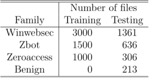
The 7-tuple scores obtained from the HMM are used for clustering. A subset of the 7-tuple HMM scores is used as training dataset to generate a cluster model. The remaining scores are given to this cluster model to see how well the model fits these scores into different clusters. The number of samples used for training and testing are given in Table 4. Based on the resulting cluster formations we calculate a probability score for each sample that is clustered and use this probability score as a performance measure to compare𝑘-means and EM algorithms. The probability score is calculated as follows:

1. Generate a clustering model using the train dataset. 2. Using the trained model, cluster the test data.

3. Calculate cluster purity for the clusters created in Step 2.

4. For each test sample, depending on the cluster to which it is assigned and the corresponding cluster purity, compute the probability with which the sample belongs to each of the malware/benign (Winwebsec, Zbot, ZeroAccess, benign) families. That is each test sample will have four probabilities associated with it.

5. From the metadata in the malware dataset, we know the family to which each test sample actually belongs to. Now for each test sample, take the probability that is associated with its own family.

6. Take the average of probability scores obtained in Step 5.

We repeat the experiment by varying the number of clusters, 𝐾 from 2 to 15. Perform the same experiment for both EM and 𝑘-means algorithms.

Table 4: Distribution of Samples Used for Clustering Number of files

Family Training Testing

Winwebsec 3000 1361

Zbot 1500 636

Zeroaccess 1000 306

Benign 0 213

5.3.2 Clustering scores from malware trained HMM models

In this experiment, the scores from HMM models trained on malware samples are used. We train the clustering algorithm on two malware families and generate a cluster model. We then try to classify the third malware family and benign files using the trained model. An example clustering model is trained and tested as follows:

∙ Prepare a 2-D train dataset such that column 1 corresponds to Winwebsec and Zbot scores from Winwebsec trained HMM model and column 2 corresponds to Winwebsec and Zbot scores from Zbot trained HMM model.

∙ Prepare a 2-D test dataset such that column 1 corresponds to benign and Ze-roAccess scores from Winwebsec trained HMM model and column 2 corresponds to benign and ZeroAccess scores from Zbot trained HMM model.

∙ Generate a clustering model using the train dataset.

∙ Fit the test dataset with the model generated in the above step.

Next, we consider a score based on these clusters to plot the Receiver Operating Characteristic (ROC) [10] curves. the ROC curve is obtained by plotting true positive rate against false positive rate, varying the threshold through the range of data values. The region under the ROC curve (AUC) provides a convenient measure of the quality

of a binary classifier [8]. An AUC of 1.0 shows perfect classification (i.e., we can draw a threshold that will separate malware files from benign files with out any misclassification), while an AUC of 0.5 indicates that the that the classifier is no more fruitful than flipping a coin.

The basis for our score is the silhouette coefficient, as discussed in Section 4.1.3.2. Given a set of clusters, where 𝑥is an element of one, say, cluster 𝐶𝑗, to compute the score of 𝑥, we first calculate 𝑆(𝑥), the silhouette coefficient of 𝑥. Next, as discussed in Section 4.1.3, we calculate 𝑝𝑖𝑗 = 𝑚𝑖𝑗/𝑚𝑗, where 𝑚𝑖𝑗 is the number of elements of family 𝑖 in cluster 𝐶𝑗 and 𝑚𝑗 is the total number of elements in cluster 𝐶𝑗. Finally, the scoring function is defined as

score𝑖(𝑥) = 𝑝𝑖𝑗𝑆(𝑥) where score𝑖(𝑥)is the score of 𝑥 with respect to family 𝑖.

Since our test dataset has two different samples (ZeroAccess and benign), each test sample file will have two scores.

score0(𝑥) = benign score of file 𝑥

and

score1(𝑥) =ZeroAccess score of file 𝑥

We use score𝑖(𝑥)to plot the ROC curve.

Once the clustering algorithm is run on the 2-D data, we extend this experiment to include more dimensions to the train and test datasets. More details about this extended experiments are given in the Chapter 6.

5.4 SVM Implementation

In this project we used the RapidMiner [29] to run the SVM algorithm. Rapid-Miner is a software platform that provides an integrated environment for machine learning, predictive analysis, data mining etc. RapidMiner provides an easy to use web interface with several drag and drop tools to construct an SVM model. Since SVM is a supervised learning algorithm, we should pre-process the data to include the labels. We used the data labels 1 and -1 to represent the two classes of samples (malware and benign). In SVM, we train an SVM model on different malware fam-ilies and verify how well the trained model can classify new samples from the same malware families. We use the same HMM scores that we used for clustering to train and test the SVM models.

5.5 Experimental Setup

In this project, since we are dealing with malware samples, most of the experi-ments are run on a virtual machine. We used the Hyper-V virtual machine manager to configure and manage the virtual machines. Following are the specifications of host and virtual machine instances.

Host:

- Model: Lenovo Ideapad Yoga

- Processor:Intel Core i5-3337U, CPU @ 1.80GHz - RAM: 8.00 GB

- System Type: 64-bit

- Operating System: Windows 8.1 Guest 1:

- Software: Hyper-V Manager - Start-up Memory:1024 MB - System Type: 64-bit

- Operating System: Windows 8.1 Guest 2:

- Software: Hyper-V Manager - Start-up Memory:2048 MB - System Type: 64-bit

- Operating System: Ubuntu 14.10

As mentioned in Section 5.2, the HMMs are trained on opcode sequences. Ex-traction of opcode sequences from the malware and benign samples is done in Guest 2 system. Training the HMM models, clustering algorithms and SVM are performed in Guest 1 system.

CHAPTER 6 Results

This chapter provides a detailed description of the results. The first section discusses the results of EM and 𝑘-means clustering algorithms. The second section discusses the results of SVM algorithm. Finally we compare the results of clustering and SVM to see which technique gives better results.

6.1 Clustering

In this section we present and discuss the results of EM and 𝑘-means clustering algorithms. Since clustering is an unsupervised learning technique, no pre-processing is required on the data. Hence the HMM scores are directly given as input to EM and 𝑘-means algorithms.

6.1.1 Clustering results of compiler trained HMM scores

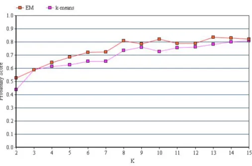
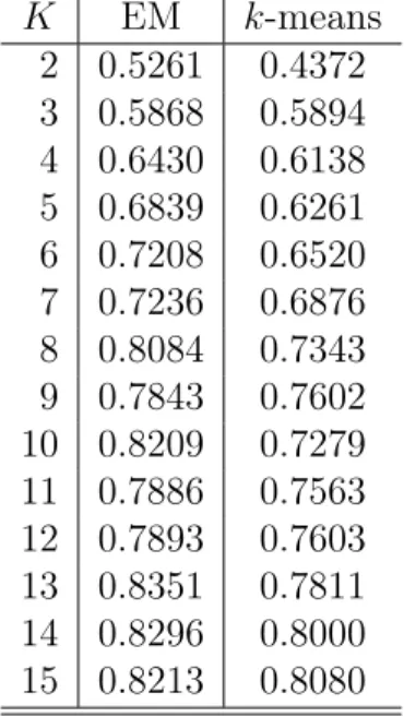
For the first experiment we consider the 7-tuple HMM scores for clustering and compute the probability score. As mentioned in Chapter 5, the probability score is computed using the metadata obtained along with the malware dataset. The clus-tering algorithm is run multiple times for the same 𝐾 and the maximum probability score of all the runs is considered for that particular 𝐾. Figure 5 shows the prob-ability score comparison of EM and 𝑘-means algorithms. The x-axis represents the number of clusters, 𝐾 and y-axis represents the probability score. The red line cor-responds to the probability scores of EM algorithm for 𝐾 = 2 to 𝐾 = 15. Similarly, the magenta line corresponds to the probability scores of 𝑘-means algorithm. The probability scores with which Figure 5 is plotted are given in Table 5.

Figure 5: Probability Score Comparison

It can be seen from Figure 5 that the probability score of EM algorithm is slightly better than 𝑘-means. That is we can say that EM clustering algorithm classifies malware samples more accurately than 𝑘-means algorithm. Also, we can observe that with increase in 𝐾 (number of clusters), there is a slight increasing trend in the probability score. This is because, as the number of clusters is more, data is grouped into more number of small but comparatively pure clusters.

6.1.2 Clustering results of malware trained HMM scores

For the initial experiment with malware trained HMM scores, we start with 2-D HMM scores (scores from two of the HMM models trained in Section 5.2.2). We perform both EM and 𝑘-means clustering algorithms on the same data with 𝐾 = 2, compute the scores as metioned in Section 5.3.2 and plot the ROC curves. Figure 6 shows the ROC curve for EM clustering algorithm for 2-D data.

Table 5: Probability Scores of EM and𝑘-means 𝐾 EM 𝑘-means 2 0.5261 0.4372 3 0.5868 0.5894 4 0.6430 0.6138 5 0.6839 0.6261 6 0.7208 0.6520 7 0.7236 0.6876 8 0.8084 0.7343 9 0.7843 0.7602 10 0.8209 0.7279 11 0.7886 0.7563 12 0.7893 0.7603 13 0.8351 0.7811 14 0.8296 0.8000 15 0.8213 0.8080

Figure 6: ROC curve for EM clustering algorithm (2-D data)

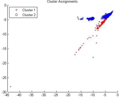
The corresponding AUC for the curve is 0.896 which implies that this clustering model can differentiate between ZeroAccess and benign files with a probability of 89.6% . The cluster formations of the ZeroAccess and benign samples using this

model are given in Figure 7, where x-axis represents the HMM scores of Winwebsec model and y-axis represents the HMM scores of Zbot model.

Figure 7: Cluster formation using EM clustering algorithm (2-D data)

Figure 8 shows the ROC curve for 𝑘-means clustering algorithm for 2-D data. The corresponding AUC for the curve is 0.81 which implies that this clustering model can differentiate between ZeroAccess and benign files with a probability of 81% . The clusters formations for the same data using 𝑘-means clustering model are given in Figure 9.

From Figures 7 and 9, we can observe that the same data samples have been put into different clusters by different clustering algorithms. Based on these different cluster formations, the two clustering models have different levels of accuracy in classifying ZeroAccess and benign samples.

For the next experiment we consider 3-D HMM scores (scores from all the three HMM models trained in Section 5.2.2). Similar to the 2-D data, we perform both EM

Figure 8: ROC curve for 𝑘-means clustering algorithm (2-D data)

Figure 9: Cluster formation using 𝑘-means clustering algorithm (2-D data) and 𝑘-means algorithms on 3-D data for 𝐾 = 2, compute the scores and plot ROC curves.

Figure 10 shows the ROC curve for EM clustering algorithm for 3-D data. The

Figure 10: ROC curve for EM clustering algorithm (3-D data)

corresponding AUC for the curve is 0.856 which implies that this clustering model can differentiate between ZeroAccess and benign files with a probability of 85.6% .

Figure 11 shows the ROC curve for 𝑘-means clustering algorithm for 3-D data. The corresponding AUC for the curve is 0.852 which implies that this clustering model can differentiate between ZeroAccess and benign files with a probability of 85.2% .

Next we consider 4-D HMM scores. The 4-D data is obtained by adding the scores of NGVCK trained HMM model to the existing 3-D dataset. We perform similar experiments on the 4-D data and plot the ROC curves.

Figure 12 shows the ROC curve for EM clustering algorithm for 4-D data. The corresponding AUC for the curve is 0.94 which implies that this clustering model can differentiate between ZeroAccess and benign files with a probability of 94% .

Figure 11: ROC curve for𝑘-means clustering algorithm (3-D data)

Figure 12: ROC curve for EM clustering algorithm (4-D data)

The corresponding AUC for the curve is 0.977 which implies that this clustering model can differentiate between ZeroAccess and benign files with a probability of 97.7% .

Figure 13: ROC curve for𝑘-means clustering algorithm (4-D data)

6.1.3 Comparison of clustering algorithms based on accuracy

In this section we compare the performance of EM and 𝑘-means clustering algo-rithms based on accuracy measure. Accuracy gives the percentage of datapoints that are correctly clustered into their specific category. Since our test dataset contains two families (ZeroAccess and Benign), accuracy gives the percentage of datapoints that are correctly classified as malware or benign. The parameters used to calculate accuracy are,

∙ TP (True Positive), is the number of malware samples correctly classified as malware.

∙ TN (True Negative), is the number of benign samples correctly classified as benign.

∙ FP (False Positive), is the number of benign samples incorrectly classified as malware.

∙ FN (False Negative), is the number of malware samples incorrectly classified as benign.

Accuracy is calculated using the formula,

accuracy= TP + TN

𝑃 +𝑁

Where,

𝑃 =TP + FN and 𝑁 =TN + FP In simple terms accuracy is given as,

accuracy= Number of correctly classified datapoints

Total number of datapoints

In an ideal case, where all the datapoints are correctly classified, we get an accuracy of 1.0. In general we want accuracy to be as close to 1.0 as possible. In this experiment we calculate the accuracy of both EM and𝑘-means algorithms by varying the value of 𝐾 from 2 to 15. Also, we perform this experiment on dataset ranging from 2-D to 7-D.

Figure 14, shows the accuracy measure of EM algorithm in which X-axis rep-resents the data dimensions varying from 2-D to 7-D, Y-axis reprep-resents the number of clusters, 𝐾 varying from 2 to 15 and Z-axis represents the accuracy value. From Figure 14, we observe that the accuracy value in all the cases is in the range of 0.8 to 1.0.

Similarly, Figure 15, shows the accuracy measure of 𝑘-means algorithm. For

𝑘-Means algorithm also we see that the accuracy values are in the range of 0.8 to 1.0. For better comparison of the accuracy values of EM and 𝑘-means algorithms, we overlap the Figures 14 and 15 to obtain 16. The stem plot in Figure 16, shows

Figure 14: Accuracy measure for EM algorithm

Figure 15: Accuracy measure for 𝑘-means algorithm

accuracy values of both EM and 𝑘-means algorithms in the same plot where the ’o’ corresponds to the accuracy value of EM algorithm and ’*’ corresponds to the accuracy value of𝑘-means algorithm. From Figure 16, we observe that with increase in𝐾, the

accuracy value of 𝑘-means algorithm is slightly greater than the EM algorithm. The main reason behind this behavior is, since Em clustering is based on the distributions in the data, eventhough we increase the value of𝐾, after a certain point the algorithm created only few data clusters and more empty clusters. On the otherhand, 𝑘-means algorithm is based on distance measure, as a result with increase in 𝐾 the algorithm created more small and pure clusters thereby giving better accuracy.

Figure 16: Accuracy comparison of EM and 𝑘-means algorithms

6.2 SVM

To perform the SVM experiments we need to first pre-process the data by as-signing data labels such that malware scores are labeled as 1 and benign scores are labeled as -1 or vice-versa.

6.2.1 SVM results of compiler trained HMM scores

Similar to the clustering experiments we initially take the 7-tuple data and per-form SVM. We use the same train and test datasets that we used for clustering. The only difference is that training dataset for clustering algorithm do not contain benign samples whereas benign samples are included in both train and test datasets of SVM. Figure 17 shows the ROC curve of SVM algorithm for 7-tuple using radial kernel function.

Figure 17: ROC curve for SVM algorithm (7-tuple data)

The corresponding AUC for the curve is 1.0 which implies that this SVM model can differentiate between malware and benign files with 100% accuracy. Also, we performed this experiment by varying the kernel functions. The kernel function and the corresponding AUC are given in Table 6.

From the AUC values in Table 6, we can observe that most kernel functions give 100% accurate SVM binary classifier.