Where does the Information in Mark-to-Market Come from?
FILL
Alexander Bleck Pingyang Gao∗ Chicago Booth
July 29, 2010
Abstract
We study the ex-ante efficiency of mark-to-market accounting (MTM) in a loan market by taking into account its real effects on banks’ origination and retention decisions. On the one hand, MTM exploits the information in asset price that improves the accuracy of asset valuation and ex-ante incentives. On the other hand, exploiting the information in asset price alters the process by which information is impounded into price and induces strategic behavior. The overall efficiency of MTM is a trade-off of these two forces. Relative to historical cost accounting, MTM could induce banks to retain excessive exposure to the risk of the loans they originate, damage price discovery in the loan market, and reduce banks’ ex-ante incentive to originate good loans. These results imply an economy with an inefficient risk distribution and a lower overall loan quality.
∗
We thank Anne Beatty, Jeremy Bertomeu, Doug Diamond, Andrei Kovrijnykh, Christian Laux, Chris-tian Leuz, Brian Mittendorf, Raghu Rajan, Korok Ray, Stephen Ryan, Haresh Sapra, Cathy Schrand, Amit Seru, Doug Skinner, Phil Stocken, Lars Stole and participants at the 2009 NBER-Sloan Project on Mar-ket Institutions and Financial MarMar-ket Risk, the Carnegie Mellon Accounting Theory Conference and the workshops at Chicago Booth and Ohio State University for valuable discussions and acknowledge financial support from Chicago Booth.
“The measurement of position necessarily disturbs momentum, and vice versa”
- Heisenberg (1929)
1
Introduction
The prevailing logic for mark-to-market accounting (MTM) is that it makes asset valuation more accurate by exploiting information in asset prices. The enhanced accuracy then generates various benefits. Notwithstanding these benefits, we show that MTM also affects firms’ behavior that determines their balance sheets MTM measures. The induced change in behavior could then inflict a cost on the economy and the overall efficiency of MTM thus involves a trade-off. In particular, in the context of a loan market, MTM could induce banks to retain excessive exposure to the risk of the loans they originate, damage price discovery in the loan market, and reduce banks’ ex-ante incentive to originate good loans, resulting in an economy with an inefficient risk distribution and a lower overall loan quality. We focus on the loan market with banks following the “originate-to-distribute” (OTD) model. Banks have expertise in originating loans but it is too costly for them to maintain the loans on their own books for various exogenous reasons. If there is no information asymmetry between banks and investors, banks pass through all the loans they originate to investors. The liquidity in the loan market is perfect and independent of accounting measurement. Accounting is then simply irrelevant. However, banks receive private in-formation about the quality of their loans because of their expertise in loan origination. Facing the lemons problem, banks rely on market mechanisms to improve price discovery in the loan market. One mechanism is for good banks (banks with good loans) to retain some portion of their loans and sell the rest at a high price. Price discovery becomes costly because it is sustained by this signaling. The cost of price discovery in turn adversely affects banks’ ex-ante incentive to originate good loans.
Accounting measurement affects the bank’s origination and retention decisions through its interaction with the costly price discovery in the loan market. We consider two polar
cases of accounting measurement: MTM and HC (historical cost). HC records the retained interest (from signaling) at its amortized cost, while MTM values it at the market price of the portion of the loan that was sold. In essence, MTM requires the early recognition of the expected economic profits or losses on the retained interest by exploiting the information in loan price.
The inefficiency of HC is obvious. HC ignores the information in loan price. In a signal-ing equilibrium, the loan price is informative about the quality of the loan. Furthermore, there seems to be a liquid market for the retained interest because the sold portion of the same loan is actively traded. Yet, HC does not allow banks to recognize the expected economic profit on the retained interest until the loan pays off. This delayed recognition increases the cost for banks to keep the retained interest on their books and reduces banks’ ex-ante incentive to originate good loans.
MTM attempts to overcome this inefficiency. By using the information in the loan price to value the retention, MTM improves the accuracy of the valuation of retained interest. All else equal (retention held constant), this enhanced valuation accuracy under MTM reduces the cost of price discovery and stimulates banks’ ex-ante incentive to originate good loans. However, switching from HC to MTM also changes the incentive for bad banks to mimic good ones and thus alters the equilibrium retention. In an attempt to exploit the information in the market price, MTM interferes with the signaling process that sustains the informativeness of the market price. It is this feedback effect that compromises the overall efficiency of MTM. In particular, we demonstrate three consequences of MTM.
First, relative to HC, MTM forces banks to retain excessive exposure to the risk of loans they originated. Even though only good banks retain a portion of the loans in equilibrium, MTM also reduces the marginal cost for bad banks to hold retained interest. Thus, good banks have to retain an even higher portion of the loan to distinguish themselves. As a result, the risk of the loan concentrates more on the banks’ own books and the loan market does not distribute the risk to investors who are better able to bear it.
destroyed under MTM. As one moves to MTM, the required retention for good banks to differentiate themselves increases. As the required retention exceeds a threshold (beyond which sales accounting is not applicable), separation becomes infeasible. In any resulting non-separating equilibrium, the market prices of loans are less informative about the quality of the loans. The attempt to exploit the information in the market price by moving to MTM destroys the informativeness of the market price.
Finally, MTM could reduce the value of originating good loans, resulting in banks’ lower ex-ante incentive to originate good loans and a lower overall quality of loans in the economy. The value of originating good loans hinges on signaling that sustains the price discovery in the loan market. MTM has two opposing effects on the cost of price discovery. On the one hand, improved valuation accuracy reduces the unit cost of holding retained interest, reducing the signaling cost. On the other hand, the early recognition under MTM also leads to higher retention in equilibrium, increasing the signaling cost. When the latter effect dominates the former, MTM increases the cost of price discovery and reduces the value of originating good loans.
The most important contribution of our paper is to provide an ex-ante evaluation of MTM relative to HC. As we will discuss in the next section, most previous studies focus on the ex-post consequences of accounting measurement. That is, given a firm’s assets, these studies examine how accounting measurement affects the decisions of the firm. Not only do we study the retention decisions given the bank’s loan portfolio, we also examine how the ex-ante origination decisions are influenced by the anticipated effects of accounting measurement. This ex-ante perspective is imperative because it is inherently difficult to evaluate the overall efficiency of a policy or system based on ex-post results in a second-best world. Taking this approach, our analysis sheds light on the role of MTM in the build-up of problems in the system that could lead to severe consequences. Such analysis could also inform the ensuing regulatory reform.
The paper also contributes to the literature on MTM by highlighting the reverse causal-ity between accounting measurement and liquidcausal-ity. As we detail in the next section, the
essence of the popular argument is often two-fold. On the one hand, MTM is theoretically justified because it enhances the accuracy of asset valuation. On the other hand, MTM may experience some implementation difficulty when asset markets are not very liquid. Valuation errors due to illiquidity in combination with the rigid reliance on accounting numbers by various parties could result in inefficient decisions that put further pressure on liquidity in asset markets, setting into motion a downward spiral. Therefore, liquidity is an important determinant of the overall efficiency of MTM. Our analysis emphasizes on the reverse causality: MTM influences banks’ behavior that endogenously determines the information and liquidity in asset markets. This interaction creates a conceptual issue for MTM and the implementation difficulty is only a symptom of this conceptual difficulty. In the model, the information in loan price and the liquidity in the loan market, liquid-ity broadly defined as the sensitivliquid-ity of market prices to banks’ (trading) behavior, are endogenous and fragile because they are sustained by the privately costly signaling. As soon as one attempts to exploit them by marking the retained interest to the market price, the signaling game changes and leads to a new balance sheet for the bank. The benefit of MTM in the form of the improvement in valuation accuracy of the balance sheet could be dominated by the endogenous cost arising from the change in the bank’s balance sheet.
The logic that how we measure a bank’s balance sheet changes the bank’s balance sheet is a general feature of accounting measurement beyond our particular model. It is reminiscent of the “Lucas Critique” that policies derived from the observed empirical re-lation could change the underlying rere-lation. The retention required to signal under MTM differs from that under HC. Therefore, it is not appropriate to predict the consequences of MTM based on the retention decisions made under HC. In general, attempting to resolve accounting measurement problems via a market-based solution could lead to unintended and sometimes undesirable consequences. While illiquidity in asset markets is the imme-diate cause, there is a deeper root of illiquidity. A firm’s business model is viable only if it has some competitive advantage over the market in conducting its activities. As a result, the core assets and liabilities on a firm’s balance sheet, dictated by its business model,
are often subject to the same market frictions that sustain the business model. Market prices in these markets are thus endogenously linked to the firm’s activities that are guided partially by accounting measurement. Accounting measurement does not only measure a firm’s balance sheet but it also actively shapes the firm’s balance sheet. This feedback loop is illustrated in Figure 1.
Figure 1: Feedback loop of accounting measurement
The rest of the paper is organized as follows. Section2reviews the literature, Section3
describes the model, Section 4 presents the equilibria, Section 5 states our main results, Section 6 considers various extensions to the basic model, and Section 7 concludes. The Appendix includes details on the accounting for securitizations (Appendix A) and the proofs that are not in the text (AppendixB).
2
Literature review
The most prominent argument about the potential cost of MTM is the procyclicality of MTM, as presented in Allen and Carletti (2008) and Plantin, Shin, and Sapra (2008). Given illiquidity in asset markets, Plantin, Shin, and Sapra (2008) show that MTM cre-ates complementarities among financial institutions’ decisions to sell their asset holdings resulting in fire sales and “artificial” volatility for assets. Allen and Carletti (2008) show that the interaction of MTM and capital requirements of financial institutions could cause contagion among otherwise independent financial sectors through the market price link.
In contrast, Laux and Leuz (2009a,b) argue that it is unlikely that MTM has contributed to or exacerbated the financial crisis for at least two reasons. First, the existing MTM accounting rules have built-in “circuit breakers” that allow banks to deviate from market prices in their books to avoid a downward spiral in the presence of illiquidity. Huizinga and Laeven (2009) provide evidence consistent with banks using MTM to hide losses during the crisis. Second, the crisis was caused by a lower quality of mortgages and the price crash in the market; hiding the loss in the crisis wouldn’t have made the situation better. The authors also call for studies on the ex-ante effect of MTM on firm behavior.
We take an ex-ante perspective by modeling the effect of ex-post accounting measure-ment on the ex-ante incentives for loan origination. As a result, we directly link MTM to the overall quality of loans in the economy and banks’ risk exposure, two factors that are often viewed as a threat to financial stability. Therefore, we respond directly to the call in Laux and Leuz (2009a) and Laux and Leuz (2009b) for studies on the ex-ante effect of MTM but reach a conclusion different from their conjecture. Further, unlike in Allen and Carletti(2008) andPlantin, Shin, and Sapra(2008), we endogenize (il)liquidity in the model. As a result, we are able to show that MTM could cause, instead of being crippled by, illiquidity. We view this as an important conceptual problem with MTM. Finally, our analysis shows that even in absence of the (rigid) regulatory use of accounting earnings, MTM could have adverse consequences for the economy. Therefore, simply severing the link between GAAP and RAP (Regulatory Accounting Principles) is no panacea to solve the problem of MTM.
Our major theoretical point that the attempt to exploit information in MTM interferes with its production is also shared by Reis and Stocken(2007) andGorton, He, and Huang
(2008). Reis and Stocken (2007) study the effect of MTM on the production and price setting behavior of firms in a duopoly. They emphasize on the point that market prices used in MTM are endogenous and transaction accounting measures are affected by the measurement. Gorton, He, and Huang(2008) study the optimal use of information gleaned from market prices of securities in solving the agency problem between a principal-investor
and an agent-trader. They show that the inclusion of market prices in the compensation contract induces traders to collude and manipulate market prices when they are able to do so.
There are other papers studying the pros and cons of MTM and HC in general. Heaton, Lucas, and McDonald(2008) study a model in which accounting as well as capital require-ments are designed to curtail banks’ risk-taking incentive. Market prices could be inefficient in this task because market prices reflect the correlation of the payoffs of assets among banks while banks’ incentive to take risk depends on the total volatility of the payoff of its own assets. Bleck and Liu(2007) point out that MTM can provide investors with an early warning mechanism while HC gives management a “veil” under which they can potentially mask a firm’s true economic performance. Their model offers a mechanism by which HC leads to higher volatility and more frequent and severe asset price crashes. O’Hara(1993) studies the consequence of MTM for banks’ choices of loan maturity and Burkhardt and Strausz (2009) models the impact of MTM on the asset substitution problem. There is also a literature on the application of MTM to hedging activities prescribed by FAS 133. One point made in some papers complements ours in that relying on MTM in the pres-ence of other frictions could alter firm behavior and lead to undesirable consequpres-ences (e.g.
Melumad, Weyns, and Ziv (1999);Kanodia, Mukherjee, Sapra, and Venugopolan (2000);
Sapra(2002)).
3
Model
Accounting measurement is inextricably connected to business transactions. Thus, we describe our model in three steps. First, we detail out the business model and the formation of the bank’s balance sheet in our model economy. Second, we specify the payoffs of players in the game. In particular, we link accounting measurement to the players’ payoffs. Finally, we describe the different rules of accounting measurement in detail.
3.1 The bank’s business model and decisions
There are three dates, t= 0,1,2, and a continuum of ex-ante identical banks. A represen-tative bank follows the originate-to-distribute (OTD) model. On the one hand, the bank has expertise in originating loans. On the other hand, it is costly for the bank to retain loans on its own books. Thus, without frictions, the bank would sell (distribute) its entire loan portfolio in the loan market.
A loan originated att= 0generates a random cash flowθe+exatt= 2. θ, the realization
of eθ, is privately observed by the bank at t = 1. θ can take two values: either good (G)
or bad (B), G > B. The ex-ante probability distribution ofθedepends on the origination
effort at t = 0, which will be detailed in the next paragraph. In contrast, the realization of ex is not revealed to anyone, including the bank, until t = 2. xe has density f(x) in [x, x], with −∞ ≤ x < x ≤ ∞, and E[ex] = 0. At t = 1, the expected cash flow of a
loan conditional on the bank’s private information is E[θe+xe|θ] =θ. Hence, we callθ the
quality (type) of a loan or interchangeably the quality (type) of the bank. This private information about loan quality is the main friction in the loan market.
The bank is financed with debt and equity. The bank’s decisions are made by the owner-manager on behalf of equity holders.1 The owner-manager assumption abstracts away from the agency issue between the management and the equity holders of the bank. Thus, the terms “bank”, “equity-holder” and “owner-manager” are interchangeable.
The owner-manager makes two decisions: the origination decision at t = 0 and the retention (distribution) decision at t= 1. At t = 0, the owner-manager exerts an uncon-tractible effort m, at a private cost ofs(m), to originate one unit of a loan. As mentioned in the previous paragraph, the effort m determines the distribution of θe. Specifically, Pr(θe(m) = G) = m. That is, a bank with origination effort m receives a good loan
1
Since it is a sequential game, the owner-manager could loose the decision rights att= 1for endogenous reasons such as the violation of covenants or regulation. In this case, the game ends at t= 1. To avoid this uninteresting case, we set up the model in such a way that the bank always survives fromt= 1to t= 2. The specific condition that ensures the survival of the bank will be detailed in footnote6when we describe the accounting treatment in detail.
(θ=G) with probability m and a bad loan (θ=B) with probability 1−m. By the law of large numbers, m also measures the average quality of loans in the economy.
The owner-manager makes the other decision, the retention decision, at t = 1 after learning its type. We assume that the bank incurs a cost c for every unit of the risky loan it carries on its books from t = 1 to t = 2. We discuss the various interpretations of cost c in Section 6 and will stick to the interpretation of c as a regulatory cost for the ease of reference in the rest of the paper. As a result of this cost c, the second part of the OTD model is at work and the bank has an incentive to sell (distribute) the loan at
t = 1. However, the retention decision is non-trivial because the bank faces the lemons problem in the loan market as a result of its private knowledge of the loan type θ,which in turn results from its expertise in loan origination (the first part of the OTD model). To overcome the lemons problem, the bank adopts a standard “skin in the game” solution. It retains k portion of the loan on its own books and investors respond with a per-unit price p(k), k ∈
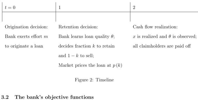
0, k, for the 1−k portion of the loan it sells.2 As a result, the bank endogenously holds a non-cash asset, the retained interest, on its balance sheet. We focus on the measurement of this endogenous asset and show that its measurement has real effects on both the bank’s retention decision att= 1 and the origination decision att= 0. At t= 2, the payoff of the loan realizes and all claimholders are paid off accordingly. There is no discounting and all parties are risk-neutral. The timing of the model is sum-marized in Figure 2.
2kis the upper limit of retention beyond which the transfer of a loan cannot be recognized as a sale
in accounting. kdoes not play any substantial role in the model but we keep it to capture this important institutional feature.
t= 0 1 2
Origination decision: Retention decision: Cash flow realization:
Bank exerts effortm Bank learns loan quality θ; x is realized andθ is observed; to originate a loan decides fraction kto retain all claimholders are paid off
and 1−k to sell;
Market prices the loan at p(k)
Figure 2: Timeline
3.2 The bank’s objective functions
At each stage of the sequential game, the owner-manager maximizes the expected present value of dividends. Denote the dividends distributed at t = 1 and t = 2 by d1 and d2, respectively. d2 is the liquidation dividend and thus includes the return of initial equity. At t= 1,the bank’s decision problem is
max k,d1,d2 d1+E h e d2 i (1)
A series of constraints are needed to link the retention decision k to dividendsd1 and d2. The first constraint is limited liability. It regulates d1 and d2 to be non-negative. Therefore, all else equal, the owner-manager prefers decisions that induce a d1 as large as possible.3 By distributing maximal dividends att= 1, the bank shifts the risk of potential future losses at t = 2 to the debt holders and essentially receives a call option on the performance of the bank’s assets. This fundamental conflict of interest between equity and
3
Of course in reality banks may not distribute dividends as much as is allowed for other reasons. Examples of such considerations include the benefit of retaining resources in the firm to absorb or hedge future liquidity needs or to capture future investment opportunities. However, even though banks may voluntarily maintain capital at a level higher than the minimum requirement (thus distribute less than is allowed in dividends), it is still true that banks (equity holders) have an incentive to distribute maximal dividends.
debt holders of the bank makes accounting measurement relevant.4 We introduce a key assumption that links accounting measurement to the bank’s behavior.
Assumption 1. The amount of dividends a bank is allowed to distribute at t= 1 cannot exceed its retained earnings at t= 1 (before dividend distribution).
We explain the consequences of Assumption 1 for our model first and then provide justifications at the end of this subsection. Assumption 1 constitutes another constraint on the retention decision problem (1). More importantly, it also connects the retention decisionkto the objective function through the link between the retention and accounting earnings, a link specified in the next subsection. We could now rewrite the objective function of the decision problem (1) at t= 1in terms of accounting earnings. Denote the accounting earnings at t = 1 and t = 2 under accounting regime A and with retention decision kby eA1 (k) andeA2 (k), respectively.
Lemma 1. Decision problem (1) is equivalent to the following decision problem max k e A 1 (k) +E max{eeA2(k),0}
The result is intuitive but significant. We can now formalize the bank’s decision prob-lems in the sequential game. The details of the proof of Lemma 1 and the claims in the following three paragraphs are provided in AppendixB.
At the final date, t = 2, the loan cash flow is realized. After all other claimholders have been satisfied, the remainder of the loan cash flow is paid to the equity holders of the bank subject to limited liability. The (equilibrium) distribution to the owner-manager is maxeA2 (k),0 .
At the interim date,t= 1, the bank sells a fractionk of its loan, revalues the retained fraction 1−k based on the accounting regime in place and recognizes earnings eA
1 (k) 4While it is beyond the scope of this paper to study other mechanisms to address this conflict, one
result from the literature is that the pricing of debt at the ex-ante stage does not resolve the ex-post conflict (e.g. Diamond and Rajan(2009)).
accordingly. The (equilibrium) distribution to the equity holders is eA
1 (k). Therefore, the bank’s retention decision problem att= 1 is summarized as
max k∈[0,k]U A(k;θ)≡eA 1(k) +E maxeeA2,0 |θ (2)
The optimum of the problem is denoted by VA(θ) ≡UA(k∗;θ), where k∗ is the optimal retention. VA(θ) is the expected equilibrium payoff to a bank of type θ. Without any friction,VA(θ)would be the same as the expected cash flow of a loan. It is (weakly) lower than the expected cash flow of a loan in our model with frictions and the wedge reflects the cost of the frictions.
At the initial date, t = 0, the owner-manager makes no dividend distribution as the bank only just originated the loan. Thus the owner-manager maximizes his expected payoff and the origination decision problem is summarized as
max
m∈[0,1]E
VA(θ(m))
−s(m) (3)
where EVA(θ(m)) = mVA(G) + (1−m)VA(B) and s(m) is the owner-manager’s private cost of exerting effort. VA(θ), the expected equilibrium payoff to a bank of type
θ, is derived from the retention problem (2) at t= 1. The two objective functions of the bank correspond to two decisions at t= 0 and t= 1, respectively, and are linked to each other consistently.
Before we turn to the description of the accounting measurement and the determina-tion of eA1(k) and eA2(k) in the next subsection, we briefly discuss Assumption 1. This assumption captures real-world intuition reasonably well. A prototype bank in our model is an insured-deposit bank. The bank issues insured debt (deposits), makes risky loans, pays the FDIC insurance premium based on its risky balance sheet, and is subject to lim-ited liability. In the event of non-performance of the loans on the bank’s balance sheet, the equity of the bank is first in line to absorb losses. However, the equity holders are not
obliged to contribute new capital or disgorge dividends previously received. As a result, the bank has an incentive to pay dividends as early as possible. To curtail such abuse of limited liability, the bank’s dividend distribution is restricted by, among other things, a capital requirement. Since the capital requirement is mainly based on accounting numbers, the amount of dividend the bank could distribute without violating the capital requirement is linked to such accounting numbers as earnings. All else equal, the higher the earnings the more freedom the bank has to distribute dividends. To the extent that the regulator could be viewed as a representative of the debt holders of the bank, the example could also be extended to other uninsured financial institutions where the capital requirement is replaced by other forms of payout restrictions, such as debt covenants.
Alternatively, we could also interpret Assumption1more broadly. What is required for our model is that accounting measurement affects the payoffs of the decision maker, being the equity holders or the manager. If there is a conflict of interest between the manager and the rest of the stakeholders of the bank as a whole and the manager of the bank has to be the decision maker (of the origination and retention decisions), then we should interpret the dividend distribution as compensation to the manager and the accounting-based re-striction on the dividend distribution in Assumption 1as an accounting-based component of compensation. In this sense, our payoff structure is also similar to that in Burkhardt and Strausz (2009); Plantin, Shin, and Sapra(2008);Bleck and Liu (2007). In the model byPlantin, Shin, and Sapra (2008), accounting is relevant because the manager’s compen-sation is tied to short-term earnings. Similarly, in Bleck and Liu (2007), the manager’s compensation is based on short-term option-like accounting numbers as in our model. The difference to our model is that both papers focus only on one phase of the transaction by assuming that the manager cares only about the first-period earnings, whereas in our model the manager cares about the entire life of the loan. While the bank’s payoff over the life of the asset is also option-like in Burkhardt and Strausz (2009), accounting again only matters in the short term in their paper.
3.3 Accounting measurement and earnings determination
The only non-cash asset on the balance of our bank is the retained interest k. The key accounting measurement issue is how we measure the value of the retained interest. We consider two polar accounting regimes: HC and MTM. Under HC, the k portion of the loan that is retained by the bank is recorded at its initial book value B0, G > B0 > B. Under MTM, the retained portion is revalued to the market price of the portion of the loan that was sold, p(k).5 In other words, MTM requires the bank to recognize the economic
profit or loss, k[p(k)−B0], at t = 1 before the loan pays off. Recall that p(k) is the per-unit price of the loan that was sold. Early recognition of the economic profit or loss on the retained portion of the loan is the main difference between HC and MTM. We include in Appendix A a detailed description of the accounting treatment for retained interests resulting from a securitization, one of the most common transactions that typically leaves banks with a retained interest, and discuss the empirical relevance of retained interests in Section6.
Now we state the determination of earnings for the first period
eA1 (k) ≡ (1−k) [p(k)−B0]−kc+e0+kB1A−B0 , A∈ {H, M} B1A = p(k) if A=M B0 if A=H
At t = 1, the bank recognizes the profit for the portion of the loan that was sold, (1−k) [p(k)−B0]. kcis the regulatory cost charge against earnings when the bank retains
k portion of the loan. e0 is the bank’s earnings from all other sources and is assumed to
5
In practice, for example in FAS 157, MTM reflects the extent to which market prices for the same or similar assets influence the valuation of an asset. For example, under MTM retained interests could be directly marked to the market prices of the homogeneous portion that has been sold. Alternatively, if there are no homogeneous assets for the retained interest, retained interests could be valued by valuation models that use inputs implied from the market prices of the sold assets that derive from the same loan pools.
satisfy e0 > c+B −B
0.6 The crux of the analysis concerns the last term. The bank recognizes the economic profit or loss on the retention by revaluing it from its initial B0 to its new book value B1A (per unit) under accounting regime A. Under MTM (A=M), the bank marks the (per-unit) book value of the retention to the market price, that is
B1A = p(k), and recognizes as earnings the capital appreciation of the retained interest,
k[p(k)−B0]. Under HC (A = H), the (per-unit) book value of the retained interest remains unchanged at its original cost B0, that is B1H =B0; the expected profit on the retained interest is not recognized at t= 1.
We turn to the earnings for the second period
e
eA2 (k;θ) ≡ k(θ+xe)−BA1, θ∈ {G, B}, A∈ {H, M}
At t= 2, when the loan pays off, eeA
2 (k;θ) is recognized as the difference between the cash flow of the retained interest and its book value. Under HC B1H = B0, so that the earnings at t= 2 equalk[(θ+xe)−B0]. In contrast, under MTMB1M =p(k), so that the earnings at t= 2 are given byk[(θ+xe)−p(k)].
Substituting the expressions foreA1 and eA2 into the retention problem (2), the bank’s objective function at t= 1 can be rewritten as follows
UA(k;θ) =p(k)−B0+e0+k(−c+θ−p(k) +Aθ) (4) where Aθ ≡ x ˆ [(x+θ)−BA 1]>0 x+θ−BA1 dF(x)− θ−B1A = BA 1−θ ˆ x BA1 −θ−x dF(x) (5)
6This sufficient condition ensures that the game does not end att= 1under any accounting regime or
retention decision, as we discussed in foonote1. The results are not affected ife0is also added to earnings of other periods.
Aθ is the option value of limited liability for the bank of type θ, θ ∈ {G, B}, under
accounting regime A, A ∈ {H, M}, and hence varies across bank types and accounting regimes.
The tradeoff driving the retention decision is clear from equation (4). The value of the retained interestkhas three components. First, the bank bears a regulatory costc, driving the bank to reduce its retention. Second, the bank receives an expected incremental payoff of θ−p(k) for the part of the fundamentals that has not been recognized as earnings at t = 1. This differential payoff across types makes signaling possible. Third, retention also gives the bank a free option Aθ and the value of this option varies across accounting
regimes and types, offsetting the cost of retention for the bank. Since banks would follow the OTD model in the absence of information asymmetry in the loan market, cost c has to be high enough to discourage retention in the benchmark case despite the option value of retention, that is,c > c1 ≡HB+1−kk(G−B). Note thatHB could be written out from
the expression ofAθ (equation (5)). We maintain this assumption aboutcthroughout the
paper.
4
Equilibrium
We use backward induction to solve the sequential game in the model.
4.1 Retention decision at t= 1
At t = 1, the bank has learned its type and chooses a retention level to convey its type to the loan market. It is a standard two-type signaling game and we use the standard definition of Perfect Bayesian Equilibrium and apply the Intuitive Criterion to select the least costly separating equilibrium as the unique equilibrium. To keep the focus on the economic discussion in the text, we refer the interested reader to Appendix B for the standard details. For the retention game, Propositions 1and 2summarize the results.
Proposition 1. Under HC, the unique equilibrium is the least costly separating equilibrium with kH(G) = G−BG+−cB−H
B and k
H(B) = 0. The per-unit prices of the loans conditional on retention are p kH(G)
=G and p kH(B)
=B. The banks’ equilibrium payoffs are VH(G) =G−B0+e0−kH(G) (c−HG) and VH(B) =B−B0+e0.
In this equilibrium, the loan price is informative about the quality of the loan. Since the loan retained on the bank’s books is homogeneous to the part sold in the market, the loan price is also informative about the quality of the retained interest. However, this informativeness of the loan price comes at a cost in that the bank with a good loan has to retain a critical fraction kH(G) of the loan on its books. This signal costs the good bank
kH(G) (c−HG).
Proposition 2. Under MTM, there are two cases. Define c2 ≡ MB+
1−k k (G−B) > c1.
Case1. If c ≥ c2, the unique equilibrium is the least costly separating equilibrium with
kM(G) = G−BG+−cB−M
B and k
M(B) = 0. The per-unit prices of the loans conditional
on retention arep kM(G)
=Gandp kM(B)
=B. The banks’ equilibrium payoffs areVM(G) =G−B0+e0−kM(G) (c−MG) and VM(B) =B−B0+e0.
Case2. If c2> c > c1, there does not exist any pure-strategy separating equilibrium. In the first case of the separating equilibrium, the bank with a good loan retains kM(G) to serve as a signal of its quality. The price discovery in the loan market again comes at a cost of kM(G) (c−MG). In the second case of c2 > c > c1, the good bank still has an incentive to separate itself from the bad bank because the benefit of separation G−B is assumed to be sufficiently large. However, the good bank could not perfectly do so because the level of retention is restricted by an upper bound ofk. We examine the second case in Section 5.3. Until then we focus on the first case where the separating equilibria are the unique equilibria under both MTM and HC.
4.2 Origination decision at t = 0
Given the equilibrium in the retention game at t = 1, the solution to the origination problem at t= 0 in (3) is simply determined by its first-order condition
VA(G)−VA(B) =s0 mbA
(6)
Recall s(m) is the private origination cost to the owner-manager. The condition has a unique interior solution if s(m) satisfies the following properties: s(0) = 0, s0(0) = 0, s0(1) =S, s00 > 0, where S is a large positive number. The most important feature of the first-order condition is that it is the expected payoff differential of good and bad loans at t= 1that determines the bank’s ex-ante incentive to exert effort. The higher the payoff differential, the higher the optimal effort mbA. Note thatmbA is also the fraction of good loans in the economy by the law of large numbers. Price discovery in the loan market drives the origination efforts by banks and thereby determines the overall quality of loans in the economy.
This link between the retention game att= 1and the origination decision att= 0is a key innovation that permits an ex-ante evaluation of MTM. Att= 0, the uncontractibility of the owner-manager’s origination effort gives rise to a moral hazard problem. The solution to the moral hazard problem relies on the information supplied by the price discovery in the loan market att= 1. This link grants significance to the standard signaling game att= 1. In a stand-alone signaling model, signaling (separating equilibrium) in general is wasteful from a social perspective and Pareto-dominated in particular when the fraction of the good type is low. Our model links the signaling game at the retention stage to the moral hazard problem at the origination stage and gives potential social value to the signaling game. Not only does accounting measurement directly affect the retention decision at t= 1, it also influences the bank’s origination efforts att= 0. This has implications for the comparison of different types of securitizations, as we will discuss in Section 6.3.
information in the loan market.
Lemma 2. When θ is public information, the accounting regime is irrelevant and banks follow the OTD model. In the unique equilibrium, the banks distribute the entire loan by setting k∗= 0. The per-unit prices of the loans are p(G) =Gand p(B) =B. The banks’ equilibrium payoffs are VA(G) =G−B
0+e0 andVA(B) =B−B0+e0. The bank exerts
first-best effort satisfying the first-order condition (6).
5
Analysis
In this Section, we analyze the economic consequences of moving from HC to MTM for banks and the loan market. Relative to HC, MTM forces banks to retain greater exposure to the risk of the loans they originated on their own books and reduces banks’ ex-ante incentive to originate good loans. We also show that MTM, in an attempt to exploit the information in the loan price, could destroy its informativeness.
5.1 MTM and banks’ exposure to risk
Proposition 3. When c≥c2, banks retain more loans on their own balance sheets under
MTM than they do under HC, that is kM ≥kH (equality for type B).
MTM induces banks to deviate further away from their OTD model. The OTD model dictates that banks distribute the risk of the loans they originated to investors who are better able to bear it. In the absence of information asymmetry in the loan market, banks therefore dispose of all of their loans regardless of the accounting regime, as in Lemma 2. However, the information asymmetry between banks and investors is an inevitable conse-quence of banks’ expertise in originating loans. In this second best scenario, the efficiency of the loan market in identifying loan quality is only sustained by good banks’ suboptimal exposure to the risk of the loans they originated. The accounting regime matters now by influencing the economic tradeoffs of the retention decision.
Proposition 3 shows that MTM leads to greater suboptimal risk retention than HC. The intuition is clear. The bad bank’s incentive to mimic drives the equilibrium reten-tion. In equilibrium, the bad bank with the equilibrium retention kA(B) = 0 receives an expected payoff of B −B0 +e0. In contrast, if the bad type mimicked the good type with kA(G), it would receive an expected payoff of UA kA(G) ;B = G−B0 +e0 +
kA(G) (−c+B−G+AB). The binding incentive compatibility condition of the bad type
equates the two expected payoffs, resulting in
1−kA(G)(G−B) =kA(G) (c−AB)
for A∈ {H, M}. Since the marginal benefit for bad banks to mimic is fixed atG−B, the equilibrium retention is determined by the bad bank’s marginal retention cost,c−AB, A∈
{H, M}.
Lemma 3. The option value of limited liability for bad banks is larger under MTM than under HC, that is MB> HB.
While holding the marginal benefit constant, early recognition of the expected economic profit on the retained position reduces the marginal retention cost for bad banks and thereby increases their incentive to mimic. As a result, good banks are forced to retain a larger position in order to distinguish themselves from bad banks.
Proposition 3 helps explain the puzzling observation that banks have maintained ex-cessive exposure to the risk of the loans they originated. This concentration of risk in the banking sector has been alleged as one of the key factors that turned the subprime mort-gage crisis into a full-fledged financial crisis. Banks retain skin in the game to overcome the information asymmetry problem in the loan market. MTM exacerbates the problem by forcing banks to put even more loans on their own balance sheets.
This costly retention affects the value of loans to banks. We examine the consequence of the loan value for the banks’ origination decision next.
5.2 Incentive to originate good loans
Proposition 4. There exists a threshold ofc, bc(defined in the proof below), above which the expected payoff of originating a good loan at t= 0is lower under MTM than it is under HC, that is VM(G)< VH(G).
Proof. Denote the value differential of a good loan under MTM and HC by∆(c).
∆(c) ≡ VM(G)−VH(G) = kH(G) (c−HG)−kM(G) (c−MG) (7) = G−B (G−B+c−MB)(G−B+c−HB) × [(G−B) (MG−HG) +MBHG−MGHB−c[MB−HB−(MG−HG)]]
As shown in Lemma 4, MB −HB−(MG −HG) > 0. Thus, ∆(c) is decreasing in c.
Further, ∆
(G−B)(MG−HG)+MBHG−MGHB [MB−HB−(MG−HG)] +ε
<0for any positiveε. Thus, if ∆(c2)<0,
VM(G) < VH(G); if ∆(c2) > 0, there exists a c∗ > c2 such that 4(c∗) = 0. For any c > c∗, 4(c) < 0. Whether ∆(c2) > 0 depends on the shape of f(x). Thus,
VM(G)< VH(G) if c >
b
c≡max{c∗, c2}.
Proposition 4 shows that MTM could reduce the value of originating good loans. In the presence of information asymmetry in the loan market, the value of owning a good loan crucially depends on the price discovery in the loan market. However, price discovery, via signaling in the model, is costly and offsets the value of originating good loans. When the informativeness of the loan price relies on the banks’ incentive to signal and MTM changes the banks’ incentive to signal, the efficiency of MTM of exploiting the information in the loan market is compromised.
Under HC, the separating equilibrium is inefficient in that banks cannot recognize the expected economic profit on the retained interest, the quality of which is fully revealed in equilibrium. MTM intends to overcome this inefficiency through early recognition based on the loan price. All else equal, MTM increases the option value of retention to compensate
good banks for bearing the retention cost. However, early recognition under MTM also increases the bad banks’ incentive to mimic. As shown in Proposition3, MTM forces good banks to retain a higher portion of the loan. As a result, the net impact of MTM on the value of originating a good loan is a tradeoff between a lower unit retention cost and a higher equilibrium retention.
This tradeoff, as highlighted in equation (7), is complicated. For example, regulatory cost c both reduces the retention level (∂kA∂c(G) < 0) and increases the unit retention. Proposition 4 shows that the balance is tilted to the detriment of MTM as c increases. The key to understanding the intuition behind Proposition 4is the following Lemma. Lemma 4. While the option value of limited liability increases for both good and bad banks when switching to MTM, it increases more for bad banks, that is MB−HB> MG−HG.
The bad bank benefits more from the early recognition under MTM because it is much closer to the threshold of limited liability if it holds the same amount of risk as the good bank. This differential change in the option value of limited liability for bad and good banks drives the result in Proposition 4.
The retention level is determined by the bad bank’s marginal retention cost c−AB
while the unit retention cost is determined by the good bank’s marginal retention cost
c−AG. When switching from HC to MTM, the reduction in the good bank’s marginal
retention cost is less than the reduction of the bad bank’s marginal retention cost. When
c is high, the level effect dominates the unit retention effect and MTM reduces the value of originating good loans.
Corollary 1. Forc >bc, banks exert less effort ex ante to originate good loans under MTM than under HC, that is mbM <mbH. As a result, the overall loan quality in the economy is lower under MTM than it is under HC.
5.3 Information and liquidity under MTM
Moving to MTM increases the equilibrium retention of loans. Since retention is restricted to k at most, signaling becomes impossible when the required retention exceeds k. This happens when the direct costc is mild and thus fails to deter bad banks from mimicking. Proposition 5. For c2 > c > c1, there does not exist any pure-strategy separating
equilib-rium under MTM. In contrast, there is a unique pure-strategy separating equilibequilib-rium under HC.
In an attempt to “correct” the inefficiency of HC by exploiting the informativeness of the loan price, MTM destroys the information in the loan price. This paradoxical result highlights the main theoretical point of the paper. In the presence of market frictions, the informativeness of the asset price is fragile in that it is sustained by a costly under-lying market process. The attempt to extract information from the asset price makes the underlying process costlier and in the extreme destroys the informativeness of the price.
This theoretical observation is of particular importance to accounting. Accounting is always an integral part of a firm’s institution and serves to fulfill a firm’s business model. A firm’s business model is viable only if the firm has some competitive advantage over the market in conducting its activities. In other words, a firm operates in areas where market frictions are present. Since which assets and liabilities a firm holds on its balance sheet is mainly dictated by its business model, it is unlikely that a firm’s core assets and liabilities, which accounting is designed to measure, are actively traded in frictionless markets. Therefore, when we contemplate on the effect of accounting rules, such as MTM, it is important to put the issue in the context of a firm’s business model and the accompanying market imperfections.
Since accounting is designed to cope with the frictions in the market, one should be cautious not to over-rely on the market to solve problems in accounting. So far, the debate about MTM focuses almost exclusively on the exogenous liquidity in asset markets. Many commentators have observed that there are no active markets for a bank’s assets
and liabilities and consequently expressed concerns about applying MTM under those circumstances.
Our model goes one step further. Not only does accounting passively respond to the exogenous liquidity, we also show that accounting could actively influence the provision of information and liquidity in asset markets. In fact, even if there appears to be an active market, applying MTM may be detrimental to the functioning of this market and could have unintended consequences both for the information and the liquidity in this market. We emphasize two such effects.
First, the informativeness of the loan price is sustained by the costly signaling of the good bank and could disappear under the pressure from MTM. Marking the retained interest to the market price makes it more costly for the good bank to send a signal relative to HC. The higher cost reduces the incentive to supply information to the market and the information in the loan price vanishes in the extreme.
Second, MTM directly influences market liquidity leaving it extremely fragile. Before applying MTM, there is an active market that trades the 1−k portion of the same loan. Since the retained securities are identical to those traded in the market, it therefore seems “indisputable” that an active market for the retained interest exists. Therefore, one may argue that MTM should be preferred for the valuation of the retained interest. The exis-tence of an active market for the retained interest is nonetheless an illusion for the bank. As soon as the bank starts to mark the value of the retained interest to the market price, the loan market responds. The liquidity in the loan market is endogenously linked to the bank’s activities. Not only does MTM measure the bank’s balance sheet, it also actively shapes the bank’s behavior that eventually determines the bank’s balance sheet.
6
Discussion and Extensions
The basic model illustrates the point that the attempt to exploit the information in asset price interferes with the market mechanism that sustains the informativeness of price in
the first place. It is this feedback effect that could compromise the efficiency of MTM and other market-based policies. In this Section, we discuss the robustness of the model to various alternative specifications and provide justifications for some key assumptions.
6.1 Interpretations of retention cost c
Cost c plays a crucial role in the model. Conceptually, c reflects the cost excess for the bank, relative to other parties, to hold the loan. In the past three decades, the bank-ing business model has been shiftbank-ing from the traditional “originate-to-hold” model to the “originate-to-distribute” model (e.g. Bernanke (2008)).7 This shift is driven by the rel-ative cost of financing loans with internal versus external capital. Berger, Kashyap, and Scalise (1995) “emphasizes regulatory changes and technical and financial innovations as the central driving forces behind transformation of the industry”. Deregulation has in-creased competition in deposit markets and inin-creased the cost to fund loans with deposits; technical and financial innovations reduce the cost to obtain funds from the loan market. As the internal cost of capital increases and external cost of capital decreases, it becomes more likely that the bank that originates the loan is not the best party to hold the loan. We capture this driving force behind the OTD model by assuming that the bank, relative to investors in the loan market, incurs an extra cost cfor retaining a unit of risky asset on its balance sheet.
One interpretation of the cost c is the regulatory cost imposed on regulated financial institutions. It could be thought of as the assessment charged by the Federal Deposit Insurance Corporation (FDIC) in the United States, which is a function of the risk of a bank’s balance sheet. Alternatively, a typical capital requirement stipulates that banks set aside a capital reserve for the risky assets on their balance sheets. c reflects the marginal
7
By the second quarter of 2008, the outstanding balance of asset-based securities (ABS), including both mortgage and non-mortgage related ABS, is estimated to be $10.24 trillion in the United States and $2.25 trillion in Europe, with an issuance of $3,455 billion in the U.S. and $652 billion in Europe in 2007, according to SIFMA data. Securities Industry and Financial Markets Association (SIFMA),http: //www.sifma.org/research/pdf/2008-08_ESF_Q2.pdf. In addition, banks also distribute loans through the syndicated loan market and the secondary loan market, which had an annual volume exceeding $1 trillion in the past few years.
cost for the bank to meet the capital requirement when they take on one more unit of a risky asset. Capital requirements have figured prominently as a motive for loan sales (e.g.
Dewatripont and Tirole (1995)).
For unregulated financial institutions, the cost c could correspond to any cost differ-entials for them and investors to fund loans. For example, c could be interpreted as the cost associated with the lack of diversification when a financial institution retains all of the loans it originates on its own books (e.g. Leland and Pyle (1977)). For another example,
c could reflect the relative expertise or investment opportunity of the financial institution and investors in the loan market. The financial institution has a competitive advantage in originating loans but other parties (investors) have a competitive advantage in managing the loans; similarly, the financial institution has other profitable investment projects but faces a financial constraint while investors have idle capital (e.g. Gorton and Pennacchi
(1995)).
6.2 Other alternatives to improve the efficiency of MTM
Given the possible inefficiency of MTM, an interesting question is whether measures to improve its efficiency exist either in the hands of the regulator or the bank? When c is interpreted as a regulatory cost, one might naturally wonder if regulators could improve the efficiency of MTM by linkingcto such observable bank characteristics as the retention level. The optimal design of cin a general setting is apparently beyond the scope of this paper. Instead, with the interpretation ofcas the FDIC assessment, if we assume that regulators are subject to the same budget constraints under HC and MTM, then, a combination of MTM and any assessment rule that links c to the retention does not qualitatively change the trade-off of MTM. The intuition is as follows. Indexing c to the retention is based on the same idea as MTM, namely to exploit the information in loan price. Since regulators have the same information problem investors face, the change in c cannot be set as a function of the bank’s true type and instead has to be imposed uniformly. Since bad banks benefit more from early recognition, the differential benefit still exists after the regulators
increase c for both banks and indexing c to retention k could exacerbate the problem in the same way MTM does.
Banks could take some measures to exploit the information in the retention. For example, banks could resell, hedge, or collateralized the retained interest after its quality has been established by the signaling game. These issues do not arise in our model because it only spans two periods but would if we allowed for a more elaborate model. However, conceptually these measures share the same idea of exploiting the information in the loan market. We conjecture that the essence of the arguments in the previous paragraph still applies. There is no free information when information has to be sustained by a costly private action.8
6.3 Pre-commitment vs. ex-post discretion in loan distribution
In our model banks choose the retention after they learn about the quality of their loans, resulting in ex-post inefficiency of dissipative signaling. An alternative is for banks to use pre-committed retention whereby banks pre-commit to a retention level before they originate loans. An apparent drawback of this pre-commitment is that nothing could prevent the banks from deviating from the commitment after they learn the information ex post. More subtly, discretionary ex-post retention dominates pre-committed retention when the moral hazard problem in loan origination is severe. The intuition highlights the novel feature of our model that information revealed through ex-post signaling is useful in resolving the moral hazard in the origination effort. Thus, the value of ex-post signaling is greater the more severe the moral hazard problem in the origination. Therefore, the severity of moral hazard in loan origination is an important predictor of the bank’s choice of securitization methods.
8
From a theoretical perspective, there is a vast literature on how to address this commitment issue in signaling games (e.g. Admati and Perry(1987);Nöldeke and Van Damme(1990);Swinkels(1999)).
6.4 Relevance of “skin in the game”
We use “skin in the game” to motivate the rationale for holding retained interest and then study the effect of accounting measurement of retained interest. While it is still debated whether “skin in the game” actually worked as intended, there is both theoretical and empirical support for this assumption. Retaining partial interests by the bank could be a solution to both its information advantage over investors or its unobservable incentive to improve the value of loans (e.g. Leland and Pyle (1977); Gorton and Pennacchi (1995);
DeMarzo and Duffie (1999); Gorton, He, and Huang (2008)). There is also empirical evidence indicating that banks do have private information and use retention as a signal (e.g. Simons (1993); Sufi (2007); Loutskina and Strahan (2008); Keys, Mukherjee, Seru, and Vig (2009)). Further, retained interest is typically a large component on a bank’s balance sheet and exerts important influences on a bank’s income statement. Using the data from Schedule HC-S in Y-9C reports that U.S. bank holding companies file quarterly with the Federal Reserve,Chen, Liu, and Ryan(2008) report that on average the value of interest-only strips and subordinated asset-backed securities, two components of retained interests, accounts for about 11% of the outstanding principal balance of private label securitized loans. The information about a bank’s position in retention interest is also available from SEC filings (e.g. 10-Q and 10-K) if the position is material.
6.5 Middle ground: Lower of Cost or Market
Our analysis relies on the comparison of two accounting regimes in their pure forms. In the model, book values under MTM rely solely on current information extracted from market prices while book values under HC do not at all. This choice of pure accounting regimes is intentional to underscore the main theoretical point of the paper. In reality, HC is often implemented using information from market prices in some circumstances in the form of the so-called lower-of-cost-or-market rule (LCM). LCM requires a downward revaluation of the book value of an asset from its current book value but does not allow an upward
revaluation. In other words, relative to HC, LCM requires the early recognition of losses (and is thus also known as HC with impairment). Note that in our model LCM would behave in the same manner as HC because the early recognition of losses is not an issue. Rather, the inefficiency in our model under HC manifests itself as the undervaluation of retained interest and this undervaluation issue would still exist under LCM.
6.6 Proportional retention and optimal security design
We model the retention as a proportional holding to circumvent the issue of optimal security design. In general, the optimal securities that should be retained as skin in the game are those that are most sensitive to the seller’s private information (Innes (1990); DeMarzo and Duffie (1999); Fender and Mitchell (2009)). Proportional retention is optimal only in certain environments. However, endogenizing the security design in our model creates additional complexity. One issue is that the optimal security design provides banks another way for differentiation. How accounting measurement interacts with the optimal security design is an interesting topic in and of itself. Another issue regarding introducing optimal security design is that it requires the endogenous specification of the regulatory cost c, which is an important component of the payoff of the retention. We leave this extension to future research.
7
Conclusion
In this paper, we propose a new mechanism by which MTM could impose inefficiency on banks. We show that, relative to HC, MTM could induce banks to retain excessive exposure to the risk of the loans they originated and reduce banks’ ex-ante incentive to originate good loans. These results derive from the main theoretical insight of the paper. In the presence of market frictions, the informativeness of the asset price is fragile in that it is sustained by an underlying market process. The attempt to extract information from the asset price makes the underlying process costlier and in the extreme destroys the
informativeness of the price. It is this feedback effect that compromises the efficiency of MTM and causes damage to the real economy. Our paper underscores that information and liquidity in asset markets are not exogenous. Rather, they are determined by the incentives and ability of market participants to overcome market frictions. Accounting measurement changes these incentives. Understanding the interplay between accounting measurement and the market process that deals with the market friction is thus of importance if we are to improve the functioning of markets with frictions.
References
Admati, A., andM. Perry(1987): “Strategic Delay in Bargaining,” Review of Economic
Studies, 54(3), 345–364. 28
Allen, F., and E. Carletti (2008): “Mark-to-Market Accounting and Liquidity
Pric-ing,” Journal of Accounting and Economics, 45(2-3), 358–378. 6,7
Berger, A., A. Kashyap, and J. Scalise (1995): “The Transformation of the US
Banking Industry: What a long, strange Trip it’s been,”Center for Financial Institutions Working Papers. 26
Bernanke, B. (2008): “Addressing Weaknesses in the Global Financial Markets: The
Report of the President’s Working Group on Financial Markets,” Speech. Virginia Global Ambassador Award Luncheon, World Affairs Council of Greater Richmond, April. 26
Bleck, A., and X. Liu (2007): “Market Transparency and the Accounting Regime,”
Journal of Accounting Research, 45(2), 229–256. 8,14
Burkhardt, K., and R. Strausz (2009): “Accounting Transparency and the Asset
Substitution Problem,” The Accounting Review, 84(3), 689–713. 8,14
Chen, W., C. Liu, and S. Ryan (2008): “Characteristics of Securitizations that
Deter-mine Issuers’ Retention of the Risks of the Securitized Assets,” The Accounting Review, 83, 1181. 29
DeMarzo, P., and D. Duffie (1999): “A Liquidity-Based Model of Security Design,”
Econometrica, pp. 65–99. 29,30
Dewatripont, M., and J. Tirole (1995): The Prudential Regulation of Banks. MIT Press. 27
Diamond, D., andR. Rajan(2009): “Fear of Fire Sales and the Credit Freeze,” Working
Fender, I., and J. Mitchell (2009): “Incentives and Tranche Retention in
Securitiza-tion: A Screening Model,” Working paper, BIS. 30
Gorton, G., P. He, andL. Huang(2008): “Monitoring and Manipulation: Asset Prices
When Agents are Marked-to-Market,” Working paper, Yale University. 7,29
Gorton, G., and G. Pennacchi (1995): “Banks and Loan Sales Marketing
Nonmar-ketable Assets,” Journal of Monetary Economics, 35(3), 389–411. 27,29
Heaton, J., D. Lucas, and R. McDonald (2008): “Is Mark-to-Market Accounting
Destabilizing? Analysis and Implications for Policy,” Working paper, University of Chicago. 8
Huizinga, H., andL. Laeven(2009): “Accounting Discretion of Banks During a
Finan-cial Crisis,” Working paper, IMF. 7
Innes, R. (1990): “Limited Liability and Incentive Contracting with ex-ante Action Choices,” Journal of Economic Theory, 52(1), 45–67. 30
Kanodia, C., A. Mukherjee, H. Sapra, and R. Venugopolan(2000): “Hedge
Dis-closures, Futures Prices, and Production Distortions,” Journal of Accounting Research, 38, 53–82. 8
Keys, B., T. Mukherjee, A. Seru, and V. Vig (2009): “Financial Regulation and
Securitization: Evidence from Subprime Loans,”Journal of Monetary Economics, 56(5).
29
Laux, C., andC. Leuz(2009a): “The Crisis of Fair Value Accounting: Making Sense of
the Recent Debate,” Accounting, Organizations and Society, 34. 7
(2009b): “The Role of Fair Value Accounting in the Financial Crisis,” Working paper, University of Chicago. 7
Leland, H., andD. Pyle(1977): “Informational Asymmetries, Financial Structure, and
Financial Intermediation,” Journal of Finance, 32(2), 371–387. 27,29
Loutskina, E., and P. Strahan (2008): “Informed and Uninformed Investment in
Housing: the Downside of Diversification,” Working paper, University of Virginia. 29
Melumad, N., G. Weyns, andA. Ziv(1999): “Comparing Alternative Hedge
Account-ing Standards: ComparAccount-ing Alternative Hedge AccountAccount-ing Standards: Shareholders’ Per-spective,” Review of Accounting Studies, 4, 265–292. 8
Nöldeke, G., and E. Van Damme (1990): “Signalling in a Dynamic Labour Market,”
Review of Economic Studies, 57(1), 1–23. 28
O’Hara, M.(1993): “Real Bills Revisited: Market Value Accounting and Loan Maturity,”
Journal of Financial Intermediation, 3, 51–76. 8
Plantin, G., H. Shin, and H. Sapra (2008): “Marking-to-Market: Panacea or
Pan-dora’s Box,” Journal of Accounting Research, 46(2), 435–460. 6,7,14
Reis, R., and P. Stocken (2007): “Strategic Consequences of Historical Cost and Fair
Value Measurements,” Contemporary Accounting Research, 24(2), 557–894. 7
Sapra, H.(2002): “Do Mandatory Hedge Disclosures Discourage or Encourage Excessive
Speculation?,” Journal of Accounting Research, 40, 933–964. 8
Simons, K. (1993): “Why do Banks Syndicate Loans?,” New England Economic Review
of the Federal New England Economic Review of the Federal Reserve Bank of Boston, January/February, 45 52. 29
Sufi, A. (2007): “Information Asymmetry and Financing Arrangements: Evidence from
Syndicated Loans,” Journal of Finance, 62(2), 629–668. 29
Swinkels, J. M.(1999): “Education Signalling with Preemptive Offers,” Review of
Appendices
A
Accounting Treatment for Retained Interest in
Securitiza-tions
In general, the shift from HC to MTM has accelerated during the past decade. This appendix describes the accounting for retained interests of securitizations.
Conditional on sales accounting, FAS 140 stipulates the accounting treatment on the transaction date. The subsequent revaluation depends on how the retained interest, a security, is classified. Securities can be classified as trading, available-for-sale (AFS), or held-to-maturity (HTM), with different accounting treatments (FAS 115 and FAS 157). The only restriction FAS 140 imposes on subsequent classification is that prepayment-sensitive securities be classified as either trading or AFS. For simplicity, we assume that the loan is measured at cost before the transaction.
On the transaction date, items could be classified into two overlapping categories for ac-counting purposes: proceeds received and retained interest. Proceeds received include cash and any other assets obtained, such as derivatives received that do not use the transferred assets as underlying assets. Liabilities incurred, including recourse commitments, are both proceeds and retained interest. Other retained interests include interests in transferred assets, such as proportional holding, interest-only strips (IO), subordinated securities, and Mortgage Servicing Rights (MSRs).
For accounting purposes, retained interests that are not proceeds are recorded at pro-rated cost at inception (the proration is based on fair value). The rationale is that the firm has not relinquished its control over these assets and therefore these are not considered to have been sold yet. However, this rationale is overwritten when the retention is classified as an AFS or trading security and thus FAS 115 and FAS 157 apply.
The proceeds are fair valued at inception. The firm receives these assets or assumes these liabilities as considerations for the sale. FAS 156 requires the fair value option for MSRs at inception (afterwards firms can choose whether to measure MSRs at impaired cost or fair value) and therefore treats MSRs as proceeds. FAS 166 further requires that all assets obtained and liabilities incurred in a securitization be initially measured at fair value. Thus, for accounting purposes, there are no retained interests that are not proceeds after FAS 166.
Subsequently, the accounting treatment of retained interests as well as the proceeds depends on their classification. FAS 140 does not directly govern the classification; instead, FAS 115 and FAS 157 apply. The only requirement of FAS 140 is that prepayment-sensitive securities could not be classified as HTM. It can only be prepayment prepayment-sensitive if the underlying loans are subject to prepayment (e.g. residential mortgages but not commercial mortgages). Therefore, not only the retained interests but also the proceeds could be revalued either at impaired cost or at fair value. Most big banks choose fair value. The incurred liabilities could be subject to FAS 5 Loss Contingency.
The transferability of the retained interests is typically not restricted in securitizations. Banks could transfer the retained interests, including selling MSRs or securitizing the IOs. This transferability does not contradict skin in the game. If the retention was previously used for signaling, banks wouldn’t be able to sell it at a price commensurate with “high retention”. As a result of this transferability and the FAS 140’s requirement that prepayment-sensitive retained interests couldn’t be classified as HTM, retained interests are rarely classified as HTM.
B
Proofs
Proof of Lemma 1
The bank at t = 0 starts with an initial equity r that satisfies the minimum capital requirement, no retained earnings, and a debt (deposits) D that pays an interest rate normalized to zero. For simplicity, all cash receipts or outlays take place at t= 2. Recall from the text that d1 and d2 are the dividends for periods 1 and 2, respectively. For simplicity, we also include in d2 the liquidation of initial equity at t = 2. The bank’s retention decision could be written as follows
max k,d1,d2 d1+E h e d2 i (8) s.t. d1 ≥0, d2≥0 (9) d1 ≤ max{e1(k),0} (10) B0 = D+r (11) e1+e2 = θ+x−ck−B0+e0 (12) d2 = max θ+x+e0−ck−d1−D,0 (13)
We prove that this dividend-based program is equivalent to the following earnings-based program
max
k e1(k) +E[max{ee2(k),0}]
We omit index A because the proof does not depend on the accounting regime. Con-straint (9) captures the bank’s limited liability: the dividend distribution cannot be neg-ative. Constraint (10) applies Assumption1 that d1 cannot exceed the retained earnings at t= 1 before dividends (because the initial retained earnings is assumed to be zero). As discussed in footnotes1and6, we have assumed thatmax{e1(k),0}=e1(k)to avoid the uninteresting case that the game ends att= 1.Thus, constraint (10) becomesd1 ≤e1(k). In equilibrium, this constraint must hold with equality because otherwise the bank could