International Journal of Production Research, Volume 46, Issue 18, 2008, pp 5075-5095
A robust kernel-distance multivariate control chart using support
vector principles
F. Camci
†, R. B.
Chinnam
*‡, and R. D. Ellis
‡†
Impact Technologies, LLC, 200 Canal View Boulevard, Rochester, NY 14623
‡
Department of Industrial & Manufacturing Engineering, Wayne State University, Detroit, MI 48201, USA
Abstract
It is important to monitor manufacturing processes in order to improve product quality and reduce production cost. Statistical Process Control (SPC) is the most commonly used method for process monitoring, in particular, making distinctions between variations attributed to normal process variability to those caused by ‘special causes’. Most SPC and multivariate SPC (MSPC) methods are parametric in that they make assumptions about the distributional properties and auto-correlation structure of in-control process parameters, and if satisfied, are effective in managing false alarms/positives and false negatives. However, when processes do not satisfy these assumptions, the effectiveness of SPC methods is compromised. Several non-parametric control charts based on sequential ranks of data depth measures have been proposed in the literature, but their development and implementation have been rather slow in industrial process control. Several non-parametric control charts based on machine learning principles have also been proposed in the literature to overcome some of these limitations. However, unlike conventional SPC methods, these non-parametric methods require event data from each out-of-control process state for effective model building. This paper presents a new non-parametric multivariate control chart based on kernel-distance that overcomes these limitations by employing the notion of one-class classification based on support vector principles. The chart is non-parametric in that it makes no assumptions regarding the data probability density and only requires ‘normal’ or in-control data for effective representation of an in-control process. It does however make an explicit provision to incorporate any available data from out-of-control process states. Experimental evaluation on a variety of benchmarking datasets suggests that the proposed chart is effective for process monitoring.
I. Introduction
In order to improve product quality and reduce production cost, it is necessary to detect equipment malfunctions, failures, or other special events as early as possible. For example, according to the survey conducted by (Nimmo 1995; Chen, Kruger et al. 2004), the US-based petrochemical industry could save up to $10 billion annually if abnormal process behavior could be detected, diagnosed and appropriately dealt with. By monitoring the performance of a process over time, statistical process control (SPC) attempts to distinguish process variation attributed to common causes from variation attributed tospecial causes, and hence, forms a basis for process monitoring and equipment malfunction detection (Martin, Morriset al.1996). It is also the most commonly used tool to analyze and monitor processes (Eickelmann and Anant 2003).
Most SPC methods are parametric in that they make assumptions about the distributional properties and auto-correlation structure of in-control process parameters, and if satisfied, are very effective in managing false alarms/positives and false negatives. Among others, they offer the following statistical and practical advantages: 1) only data from an in-control state is necessary to initialize the control chart, 2) data from a relatively limited number of sub-groups (say 20 to 30) is adequate for accurate initialization, and 3) tradeoffs between false alarms/positives (Type-I error) and false negatives (Type-II errors) can be managed (by changing the width of the control limits and the sub-group sample size, respectively). While conventional SPC charts (such as the Shewhart type control charts (Shewhart 1926), the cumulative sum (CUSUM) control charts, and the exponentially weighted family control charts) are developed for univariate processes (Manabu, Shinjiet al.2004), multivariate statistical process control (MSPC) is employed to monitor processes that have correlated multi-variables (Montgomery 2001). One type of MSPC is multivariate charts extended from univariate SPC methods, including Hotelling’s 2
T chart (Hotelling 1947), multivariate EWMA (Lowry, Woodall et al. 1992); (Runger and Prabhu 1996), (Testik and Borror 2004) and multivariate CUSUM charts (Ngai and
Zhang 2001); (Runger and Testik 2004). Another type of MSPC is based on latent variable projection, such as Principal Component Analysis (PCA) and Partial Least Squares (PLS) (MacGregor and Kourti 1995) (Raich and Cinar 1996) (Yoon and MacGregor 2004). An alternative approach to account for the dynamic aspects of the data in MSPC is to use MRA (multi-resolution analysis) (Bakshi 1998; Teppola and Minkkinen 2000). For a good review of MSPC charts, see (Lowry and Montgomery 1995). Among these, Hotelling’s 2
T chart is widely used in practice (Sun and Tsung 2003).
The standard assumption behind majority of SPC and MSPC methods mentioned above is that the process variables follow a Gaussian distribution (Rose 1991), a questionable assumption in several industrial processes (Polansky 2001), and in particular, highly automated processes (Chinnam and Kolarik 1992). (Schilling and Nelson 1976) and many other researchers have investigated the effects of non-normality on the control limits and charting performance. To alleviate such effects, some distribution-free ornon-parametriccontrol charts have been proposed based on sequential ranks of data depth measures (Liu and Singh 1993; Aradhye, Bakshi et al. 2001; Stoumbos and Reynolds 2001; Chakraborti, Van der Laanet al.2003; Messaoud, Weihs et al. 2004), but their development and implementation have been rather slow in industrial process control (Chakraborti, Van der Laanet al.2001).
Several non-parametric control charts based on machine learning and pattern recognition principles have also been proposed in the literature. For example, (Cook and Chiu 1998) proposed radial basis function (RBF) networks to recognize shifts in correlated manufacturing processes, (Chinnam 2002) proposed support vector machines (SVMs) for recognizing shifts in correlated and other manufacturing processes, and (Smith 1994) and (Pugh 1991) considered multi-layer perceptron (MLP) networks for implementing Shewhart type control charts, all relaxing the Gaussian assumption. While these methods have shown success in relaxing the Gaussian assumption, the fundamental limitation with these and most other machine learning methods
‘classification’ or ‘pattern recognition’, and hence, strictly require example data from all out-of-control states of interest. This is a critical limitation for obtaining example cases from all such states might be difficult, expensive, or even impossible. The second limitation is that they make no explicit provision to make tradeoffs between Type-I errors (false alarms) and Type-II errors (inability to detect shifts in process condition). Most of these machine learning methods also necessitate modeling and training for each specific failure type. A model that is developed for a specific type abnormal event (out-of-control state) cannot necessarily give good classification accuracy for another type of abnormal event.
This paper presents a new non-parametric kernel-distance control chart that employs the notion of one-class classification or novelty detection to overcome these limitations and adopts support vector machine (SVM) principles for doing so. There are several reasons for basing the proposed control chart on SVM principles: 1) They are a system for efficiently training linear learning machines in the kernel-induced feature space, 2) they successfullycontrolthe flexibility of kernel-induced feature space through generalization theory, and 3) they exploit existing optimizationtheory in doing so. An important feature of SVM systems is that, while enforcing the learning biases suggested by generalization theory, they also produce ‘sparse’ dual representations of the hypothesis, resulting in extremely efficient algorithms (Cristianini and Taylor 2000). This is due to the Karush-Kuhn-Tucker conditions (Kuhn and Tucker 1951) (Mangasarian 1994), which hold for the solution and play a crucial role in the practical implementation and analysis of these machines. Another important feature of the support vector approach is that due to Mercer’s conditions on the kernels (Mercer 1909), the corresponding optimization problems are convex and hence have no local minima. This fact, and the reduced number of non-zero parameters, marks a clear distinction between these systems and other machine learning algorithms, such as neural networks (Cristianini and Taylor 2000). The end result is that the proposed kernel-distance control chart is non-parametric, only requires data from
states, and allows some tradeoff between Type-I and Type-II errors. The proposed kernel-distance control chart supports both univariate and multivariate processes and can monitor both process location and dispersion aspects through a single control chart.
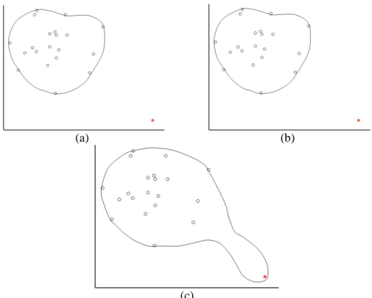
A notable exception in the literature that also offers several similar features is another kernel-distance control chart (called k-chart) independently proposed by (Sun and Tsung 2003), also based on a one-class classifier, Support Vector Data Description (SVDD), developed by David Tax (Tax 2001; Tax and Duin 2004). However, a significant limitation with SVDD, and hence the k-chart by Sun and Tsung, is that it lacks any ability to make a good distinction between outliers and normal data within the training set. In addition, they make no provision to utilize any available data from out-of-control states, and lastly, they offer no structured method for making tradeoffs between Type-I and Type-II errors. This can also result in poor representation of the in-control process state if the data available for initializing the in-control chart is not pre-processed for elimination of outliers. Our proposed kernel-distance control chart overcomes these limitations by integrating the SVDD method with principles borrowed from Support Vector Representation and Discrimination Machine (SVRDM) by Yuan and Casasent (2003). Many of these positive attributes of our proposed kernel distance control chart are illustrated in Figure 1. Here, we particularly work with the same multivariate process control dataset employed by (Sun and Tsung 2003). Figure 1(a) illustrates a plot of ‘normal’ process data projected onto the space of the two most dominant principal components (identical to Figures 11-12 of (Sun and Tsung 2003)), along with a known ‘outlier’ point (from Figure 13 of (Sun and Tsung 2003)). If one were to use the data from Figure 1(a) to initialize the k-chart, there is no guarantee that the outlier point will be recognized to be an outlier (see for example Figure 9 of (Sun and Tsung 2003)). On the contrary, the kernel distance control chart proposed here gives us several options. Supposing that the outlier data point is not so labeled and presented for chart initialization, the proposed method recognizes the point to be an outlier (as shown in Figure 1(a)). If the outlier point is labeled prior to chart initialization as an ‘outlier’, the proposed method recognizes this label and puts it outside
the normal boundary (as shown in Figure 1(b)). If for some reason, one chooses to treat this outlier point as a ‘normal’ data point, the proposed method will accept this constraint and treats the point as normal and defines normal process boundary with the point as a boundary point (as is evident from Figure 1(c)). Thus, the proposed kernel distance control chart is very robust and can take advantage of any available data/knowledge regarding process faults. In addition, our proposed method also offers an effective heuristic for optimizing the kernel parameters, something missing from SVDD and the k-Chart from Sun and Tsung. For all these reasons, we label the proposed method therobustkernel-distance control chart orrk-Chart in short.
(a) (b)
(c)
Figure 1. Flexibility ofrk-Chart. In Panel a) the point well outside the normal data is “unlabeled” but is
recognized and declared to be an outlier byrk-Chart. In panel (b) the point is “labeled” as an outlier, and
therk-Chart again declares it an outlier making use of the labeling. The results are identical to those
without labeling. Finally, in panel c) the point is “labeled” as normal, andrk-Chart accepts this constraint
and treats the point as normal and defines normal process boundary with the point as a boundary point. In
The rest of this paper is organized as follows: Section II provides background information on support vector machines, the theory behind rk-Chart is presented in Section III, experimental results in Section IV, and concluding remarks in Section V.
II. Support Vector Machines
This section provides a brief background on support vector machines (SVMs) rooted in Statistical Learning Theory, a notion first introduced by (Vapnik 1998). We first explain the basics of SVMs for binary classification and then discuss how the technique can be extended to deal with the problem of one-class classification for developingrk-Chart.
II.1. Binary classification – Linear case
SVMs belong to the class of maximum margin classifiers. They perform pattern recognition between two classes by finding a decision surface that has maximum distance to the closest points in the training set, which are termed support vectors. We start with a training set of points
d i
x , i1, 2...,N where each point xi belongs to one of two classes identified by the label
1, 1 iy and d is the dimensionality of the points. Let the training set be denoted by {( ,xi yi)}iN1. Assuminglinearly separabledata, the goal of maximum margin classification is to separate the two classes by a hyperplane such that the distance to the support vectors is
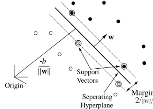
maximized. This is achieved by minimizing w2subject to the constraint yi(x wi b) 1 0, where w is normal to the hyper-plane. Figure 2 illustrates these concepts for the separable case. In order to provide fornon-separablecases, the formulation is modified as follows:
Minimize w2C
i (1)Subject to: yi
x wi b
1
i 0 (2) This quadratic optimization problem can be solved efficiently using the following Lagrangian dual formulation:Maximize , 1 2 i i j i j i j i i j y y
x x (3)Subject to: 0
iC and i. i 0 iy
(4)where
i denote the Lagrange multipliers. The Lagrangian formulation of the problem offers the advantage of having Lagrange multipliers in the constraints and training data in the form of inner products between data vectors (Müller, Mika et al. 2001). In the solution, non-zero
i values represent support vectors that are on the separating hyper-plane (satisfying the equation0 b w x ). -b ||w|| w Margin 2/||w|| Support Vectors Origin Seperating Hyperplane
Figure 2: Separation of classes by hyper-plane.
II.2. Binary classification – Nonlinear case
In many cases, classes are not linearly separable. In order to learn non-linear relations with a linear machine, we need to select a set of non-linear features and to rewrite the data in the new representation. This is equivalent to applying a fixed non-linear mapping of the data to a feature space, in which the linear machine can be used. Thus, the non-linear separable case could be handled in two steps: first a fixed non-linear mapping transforms the data into a feature space F, and then a linear machine is used to classify them in the feature space. One important property of linear learning machine is that it can be expressed in a dual representation. That is, the hypothesis can be expressed as a linear combination of the training points so that the decision rule can be evaluated using just inner products between the test point and the training points. If one could
compute the inner product ( )xi ( )x in feature space directly as a function of the original input points, it becomes possible to merge the two steps needed to build a non-linear learning machine. We call such a direct computation method akernelfunction. A kernel is a function K, such that for all x z, X
( , ) ( ) ( )
K x z
x
z (5)where
is a mapping from X to an inner product feature space F.By replacing the inner product with an appropriately chosen ‘kernel’ function, one can implicitly perform a non-linear mapping to a high dimensional feature space without increasing the number of tunable parameters, provided the kernel computes the inner product of the feature vectors corresponding to the two inputs. Thus, the use of kernels makes it possible to map the data implicitly into a feature space and to train a linear machine in such a space, potentially side-stepping the computational problems inherent in evaluating the feature map.
In practice, the approach taken is to define a kernel function directly, hence implicitly defining the feature space. In this way, we avoid the feature space not only in the computation of inner products, but also in the design of the learning machine itself. Mercer’s theorem (Mercer 1909) provides a characterization of when a function K( , )x z is a kernel (i. e. what properties are necessary to ensure that it is a kernel for some feature space). An important family of kernel functions is the polynomial kernel:
( , ) (1 )d
K x z x z (6)
where d is the degree of the polynomial. In this case the components of the mapping are all the possible monomials of input components up to the degree d. An even more popular kernel in the literature is the Gaussian (Tax and Duin 1999; Yuan and Casasent 2003):
2 2
( , )
For a good discussion on making kernels, see (Cristianini and Taylor 2000). For more detailed information on the broader topic of support vector machines see (Müller, Mika et al. 2001).
III. Robust Kernel-Distance Control Chart (rk-Chart) III.1.rk-Chart as a one-class classifier
As stated earlier, the proposed robust kernel-distance control chart (rk-Chart) employs the notion of one-class classification for process monitoring, and in doing so, models the boundary of process data from an in-control state and declares the process to be in control or out of control depending on where the new observation lies with respect to the boundary that exists in the feature space.
In the statistical process control literature, the two most important measures that are of particular interest in the context of process monitoring are measures of processcentral tendency and process dispersion. As originally proposed by W. Shewhart (Shewhart 1926), the sample arithmetic meanis the most employed measure for central tendency (among other measures such as mode and median). While the simplest statistical parameter that describes variability in observed data is the sample range, the sample standard deviation is a better estimate of variability for it considers every observation. Not unlike many multivariate statistical process control (MSPC) methods, the proposed rk-Chart jointly models these measures of central tendency as well as dispersion in a multi-dimensional space. While we recommend the sample mean and standard deviation as statistical measures for process monitoring (resulting in a 2-dimensional space), the proposed rk-Chart method is a general method and can incorporate any other type of location and dispersion measures, promising application specific measures, as well as other measures such as higher-order statistical moments (e. g., skewness and kurtosis). The only requirement for rk-Chart is that the vector of sample statistical measures is real, d
i
vectors (as well as the size of the training set) necessary for adequate representation of normal or in-control process state will increase as a function of d . In the case of multivariate processes, the feature space could simply be the process variable space or a transformation thereof (such as the space of dominant principal components). While it is also possible to introduce features from the co-variance matrix of the subgroup sample to monitor process dispersion, care should be exercised to manage d. Given that rk-Chart models the process data in two or higher dimensional spaces, in the case of univariate processes, it is necessary that the subgroup sample size be greater than one to facilitate extraction of at least two features (such as mean and standard deviation). Whilerk-Chart can in theory deal with both univariate and multivariate processes, and jointly monitors both location and dispersion measures, it does not necessarily have the ability to identify the type of process fault (such as a process location shift or process variance shift).
Thus, in developing the proposed control chart, we deviate from classical SVM designed for binary classification to representation of boundary from a single class (i. e. d
i
x ).rk-Chart is particularly inspired from Support Vector Data Description (SVDD) (Tax and Duin 1999) and Support Vector Representation Machine (SVRM) (Yuan and Casasent 2003) and gives the minimum volume closed spherical boundary around the in-control process data, represented by center c and radius r. Minimization of the volume is achieved by minimizing r2, which representsstructural error(Müller, Mika et al. 2001):
Min r2 (8)
Subject to: 2 2
i r i
x c , xi: th
i data point (9)
The formulation above does not allow any data to fall outside of the sphere. In order to make provision within the model for potential outliers within the training set, a penalty cost function is introduced as follows (for data that lie outside of the sphere):
Min 2
i i
Subject to: 2 2
i r i
x c , i 0 i (11)
where C is the coefficient of penalty for each outlier (also referred to as the regularization parameter) and i is the distance between the ith data point and the hyper-sphere. Once again,
this is a quadratic optimization problem and can be solved efficiently by introducing Lagrange multipliers for constraints (Vapnik 1998):
2 2 ( , , , , ) ( 2 ) i i i i i i i i i i i L r r C r
c ξ α γ x x c x c c (12)where i and i are Lagrange multipliers, i 0, i0, and x xi i is inner product of xi and xi. Note that for each training data point xi, a corresponding i and i are defined. L is minimized with respect to r, c, and ξ, and maximized with respect to α and γ. Taking the derivatives of (12) with respect to r, c, ξ, and equating them to zero, we obtain the following constraints:
i i i
c x (13) 0 i i C i (14) 1 i i
(15)Given thati 0,i0, constraint (14) can be rewritten as:
0i C i (16)
The following quadratic programming equations can be obtained by substituting (13), (14), (15), and (16) in (12). Max , ( ) ( ) i i i i j i j i i j
x x
x x (17) Subject to: 0i C i, i 1 i
(18)Standard algorithms exist for solving this problem (Tax 2001). The above Lagrange formulation also allows further interpretation of the values of α. If necessary, the Lagrange
multipliers (i,i) will take a value of zero in order to make the corresponding constraint term zero in (12). Thus, therk-Chart formulation satisfies the Karush-Kuhn-Tucker (KKT) conditions for achieving a global optimal solution. Noting that C i i, if one of the multipliers becomes zero, the other takes on a value of C. When a data point xi is inside the sphere, the corresponding i will be equal to zero. If it is outside of the sphere, i.e. i 0, iwill be zero resulting in i to be C. When the data point is at the boundary, i and i will be between zero and C to satisfy (15). The quadratic programming solution often yields a 'few' data points with a non-zero i value, orsupport vectors. What is of particular interest is that support vectors can
effectively represent the data while remaining sparse. Let SSV { :xi i0} denote the set of support vectors.
In general, it is highly unlikely that a hyper-sphere can offer a good representation for the boundary of in-control process data in the ‘original input space’. Hence, data ought to be transformed to a ‘higher dimensional feature space’ where it can be effectively represented using a hyper-sphere. Not unlike SVMs, rk-Chart also employs kernels to achieve this transformation without compromising computational complexity. Thus, the dot product in (17) is replaced by a Kernel function, leading us once again to the following quadratic programming problem:
Max , ( , ) ( , ) i i i i j i j i i j K K
x x
x x (19) Subject to 0i C i, i 1 i
(20)III.2. Gaussian kernel optimization withinrk-Chart
The proposed robust kernel-distance control chart employs the one-class classification formulation from above along with a Gaussian kernel. The Gaussian kernel has been shown to particularly offer better performance over other kernels for one-class classification problems (see (Tax 2001) for more discussion on this) and hence the motivation for using it. The issue is
optimization of the scale parameter of (7). While could be specified by the user, rk-Chart employs the procedure outlined in Table 1 for choosing .
Table 1: Heuristic procedure for choosing for the Gaussian kernel.
Step 1: Calculate the average 'nearest neighbor distance', denotednd, between all the data points in the
dataset (i. e. ( nnd)
d i
n E x where nnd || || || || ,
i j i k i
x x x x x i k ji E denotes
average operator over the training set).
Step 2: For each data point xi:
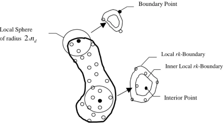
2.1: Construct a local robust kernel-distance ‘boundary’, denotedrk B- iL, utilizing the set
2 2
{ :|| || (2 ) }
i j j i nd
S x x x (i. e. data within a sphere of radius 2nd).§ In building
- L i rk B , set || ( ) || i i L i E i E i
S x S x for the Gaussian kernel (i. e. the average distance of
data within Si to the mean ofSi). Let ri* denote the optimal radius of - L
i
rk B , i. e. the
quadratic programming solution.
2.2: If xirk B- iL(ri*), i. e. the data point is rejected by a scaled orinner rk B- iLof radius
*
i
r
where 0 1 (a parameter pre-specified by the user, typically around 0.95), it is added
into theboundary list, denoted SBL. It is also necessary that for any data point to be part of
BL
S , it cannot be accepted by any other inner rk B- Lj . In addition, ifSi xi, xi is
excluded from SBL for it might be an outlier. Fig. 3 illustrates this procedure for
determination of SBL.
Step 3: The optimal global rk B- G(i. e. therk-Chart boundary that represents the complete training set
) is then constructed using the following Gaussian kernel parameter:
* min( ) max( ) arg max { ( )} nnd nnd i i BL SV x x S S .
§Tax and Duin (Tax and Duin 1999) show that this setting of the local sphere radius to 2
d
n results in good
performance.
Figure 3: Determination of class boundary list: Data points on the boundary will be rejected byinner local
rk-Boundaries.
Boundary Point
Interior Point Localrk-Boundary
Inner Localrk-Boundary Local Sphere
In the context of a globalrk-Chart, smaller values yield more representing points (i. e. support vectors) and a tighter hyper-sphere, whereas larger values give fewer support vectors and result in a bigger hyper-sphere. The goal is to identify a value for that results in good agreement between the 'support vector list' SSVof the global rk-Chart boundary and the 'boundary list' SBL
resulting from localrk-Boundaries (see Table 1 for precise definitions of these terms, and Figure 3 for a depiction of the class boundary list):
* min( ) max( ) arg max { ( )} nnd nnd i i BL SV x x S S (21)
In general, smaller values result in a global support vector list that is a superset of the boundary list, with some points that are not part of the boundary list. On the contrary, larger values result in a global support vector list that is a subset of the boundary list. In assessing this agreement, rk-Chart computes the fitness of a value by employing a two-part strategy: effective representation and compactness. Effective representation is achieved by ensuring that the global support vector list 'best matches' the boundary list. Compactness on the contrary emphasizes a smaller support vector list, which improves generalization. Compactness is managed through a user-defined parameter 0 1. The higher the value of the more compact the support vector list and the higher the Type II error (i. e. inability to detect novel conditions), resulting in a larger hyper-sphere.
There is typically a value, denoted by c, that results in near perfect agreement between the support vector list and the boundary list. As exceeds c, the support vector list gets smaller. The actual value of employed in constructing the proposed globalrk-Chart is:
( )
c max c
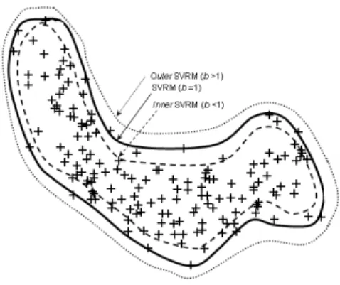
(22) Figure 4 illustrates the influence of different compactness levels on the quality of representation, using an example dataset. The innermostrk-Chart boundary provides effective representation but with 20 support vectors all of which are in SBL ( 0), whereas the outermostrk-Chart boundary
achieves compactness with just 2 support vectors ( 1). While the parameters
min min( )
nnd i
x
,max max(xinnd),c are calculated empirically, the compactness parameter
and the rk-Chart boundary scaling parameter (employed for constructing the scaled inner- iL
rk B ) need to be pre-specified by the user or require repeated trials (typically set around 0.95).
Figure 4: Influence of onrk-Chart representation.
Once the optimal value is calculated based on the desired degree of compactness, one can construct ‘inner’and ‘outer’boundary representations by correspondingly changing the radius of therk-Chart hyper-sphere. Figure 5 illustrates this procedure for the same dataset from Figure 4. It is clear that as the radius is changed the overall geometric shape is maintained while the scale changes.
Figure 5: Influence of scalingrk-Chart hyper-sphere radius (using parameter) on boundary
III.3. Learning from abnormal data
There are occasions when observation samples from abnormal or out-of-control process states are available in the training set. Not exploiting this information can have a major detrimental effect on the performance of the control chart (in terms of Type-I and Type-II errors). The earlier rk-Chart formulation can be modified as follows to exploit any available examples from out-of-control states:
Min 2 i o j
i j
r C
C
(23)Subject to: xi c r2
i and xj c r2 j (24)where Co is the penalty value for an out-of-control state data point falling inside the representation boundary.
The Lagrange formulation of this new problem is as follows:
2 2 ( , , , , ) ( 2 ) i o j i i i j i j j i i i i i j i L r r C C r
cξ α γ x x c x c c (25)To satisfy KKT condition, we once again take derivates of the cost function w.r.t. the parameters and equate them to zero, leading to the following equations:
1 i i i i
(26) i i j j i j
c x x (27)Substituting (26) and (27) in (25), leads us to following Lagrange formulation:
, , , , ( , , , , ) ( ) ( ) ( ) ( ) ( ) ( ) i i i i i i i j i j i I i J i j I i j i j i j i j i I j J i J j I i j i j i j J L r
cξ α γ x x x x x x x x x x x x (28)where, I is the class of in-control state examples and J is the class of out-of-control state examples. This formulation can be simplified by labeling out-of-state classes as '-1' and in-control class as '+1'. 1 1 i i i x I y x J (29) ' i yi i
(30)Substituting (29) and (30) in (28) results in the following:
Max ' ' ' { , } , { , } ( ) ( ) i i i i j i j i I J i j I J
x x
x x (31) 0
iC (32) 0
j Co (33) 1 i i i i
(34)As can be seen from equations (31-34), the formulation essentially remains the same with an additional constraint for the corresponding Lagrange multiplier value of the out-of-control state example.
IV. Experimental results
The application ofrk-Chart will be discussed in two subsections: First,rk-Chart is evaluated using datasets that follow common probability distributions (i. e. normal, lognormal and exponential). We then evaluate rk-Chart using a benchmarking dataset (i. e. the Smith dataset) (Smith 1994) that has been used extensively for methodological development and evaluation in the process control literature (Chinnam 2002).
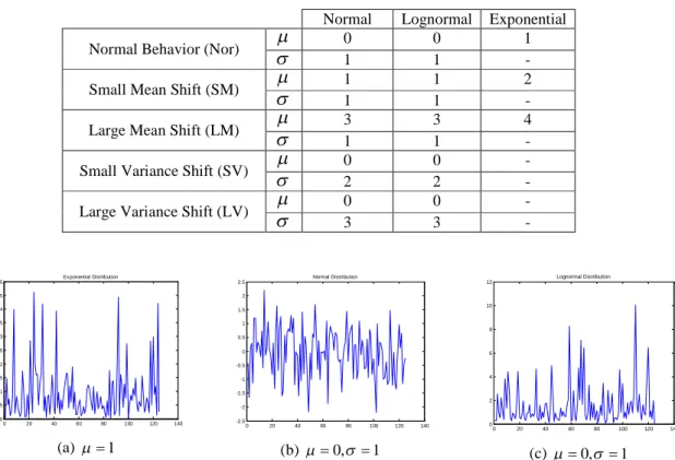
First, normal, lognormal and exponential distributions are employed to generate data. Parameters for the distributions and a sample of dataset are given in Table 2 and Figure 6, respectively. For a typical X chart, it is recommended to have at least 20-25 patterns (Woodall
and Montgomery 1999). In our experiment, 250 samples are generated for each distribution. Samples are grouped with size of 10 and two features, the mean and the standard deviation, are calculated for each sample group, resulting in only 25 two-dimensional data points.
Table 2: Parameters of distributions for evaluation experiments.
Normal Lognormal Exponential
Normal Behavior (Nor) 0 0 1
1 1
-Small Mean Shift (SM)
1 1 21 1
-Large Mean Shift (LM)
3 3 41 1
-Small Variance Shift (SV) 0 0
-2 2
-Large Variance Shift (LV)
0 0-3 3 -0 20 40 60 80 100 120 140 0 0.5 1 1.5 2 2.5 3 3.5 4 4.5 5 Exponential Distribution (a) 1 0 20 40 60 80 100 120 140 -2.5 -2 -1.5 -1 -0.5 0 0.5 1 1.5 2 2.5 Normal Distribution (b) 0, 1 0 20 40 60 80 100 120 140 0 2 4 6 8 10 12 Lognormal Distribution (c) 0, 1
Figure 6: Example time Series. a) IID Exponential, b) IID Normal, c) IID Lognormal.
We trainedrk-Chart in two ways: First, with only in-control data, and second, with in-control and limited out-of-control data as well. In the latter case, we used 10 abnormal patterns. As mentioned before, rk-Chart does not require out-of-control data, but having some helps to improve the accuracy of the method. Type-I and Type-II errors are defined as rejecting a true hypothesis and accepting a false hypothesis, respectively. In a statistical process control context, Type-I error refers to rejecting an in-control process as if it is out-of-control and Type-II error refers to accepting an out-of-control process as if it is in-control. The format of reporting Type-I and Type-II errors is given in the Table 3. The results ofrk-Chart implementation on processes that follow normal, lognormal, and exponential distributions are summarized in Table 3.
Table 3: Type-I and Type-II errors defined.
Hypothesis Test Estimated
In-control Out-of-control
A
c
tu
a
l In-control Correct Type-I error
Out-of-control Type-II error Correct
Table 4: Classification accuracy for: 1) (Left side of the table) Training only with 25 in-control patterns or sub-groups, each of which sub-group sample size of 10. 2) (Right side of the table) Training with 25 in-control and 10 out-of-in-control patterns, each with a sub-group sample size of 10; a) Normal b) Lognormal c)
Exponential distributions; SM: Small Mean Shift, SV: Small Variance Shift, LM: Large mean shift, LV: Large variance shift.
1) Training only with in-control data 2) Training with in-control and limited out-of-control data a.1 Estimated a.2 Estimated In-control Out-of-control In-control Out-of-control A ct u al In-control 88.3% 11.7% A ct u al In-control 86.6% 13.4% O u t-o f-co n tr o l SM 7.4% 92.6% O u t-o f-co n tr o l SM 9.0% 91.0% LM 0.0% 100.0% LM 0.0% 100.0% SV 6.4% 93.6% SV 4.1% 95.9% LV 0.2% 99.8% LV 0.1% 99.9% a) Normal Distribution b.1 Estimated b.2 Estimated In-control Out-of-control In-control Out-of-control A ct u al In-control 73.2% 26.8% A ct u al In-control 81.3% 18.7% O u t-o f-co n tr o l SM 4.5% 95.5% O u t-o f-co n tr o l SM 9.5% 90.5% LM 0.0% 100.0% LM 0.0% 100.0% SV 14.8% 85.2% SV 16.9% 83.1% LV 4.1% 95.9% LV 3.0% 97.0% b) Lognormal Distribution c.1 Estimated c.2 Estimated In-control Out-of-control In-control Out-of-control A c tu al In-control 88.8% 11.2% A c tu al In-control 80.8% 19.2% O u t-o f-co n tr o l SM 23.9% 76.1% O u t-o f-co n tr o lSM 16.0% 84.0% LM 0.7% 99.3% LM 0.4% 99.6% c) Exponential Distribution
As seen from Table 4, the non-parametricrk-Chart technique is able to detect out-of-control processes with no available out-of-control data with Type-I errors ranging from a highest of 26.8% to a low of 11.2%. Type-II errors ranged from 23.9% down to 0% in the case of no available out-of-control data. When limited training data from faulty process states are available,
Type-I errors improve to a high of 19.2% and a low of 13.4%. Type-II errors also improve with limited faulty process training data, to a high of 16.9% and a low of 0%.
We will also demonstrate the effectiveness ofrk-Chart for detecting mean and variance shifts in using the benchmarking dataset generated by Smith (Smith 1994) and compare the results from a general support vector machine (SVM) method proposed by (Chinnam 2002) and a multi-layer-perceptron (MLP) neural network model (Smith 1994). The dataset has 300 samples from in-control state and out-of-in-control states of large mean shift (LM), small mean shift (SM), large variance shift (LV), and small variance shift (SV). The parameters are given in Table 5. The results will be reported in three different categories. In the first category, the results of rk-Chart will be compared with results of Shewhart chart, MLP and SVM. Note that MLP and SVM create a distinct model for each abnormality type (e.g. small mean shift, large variance shift). In the second category, two different rk-Chart results are reported: rk-Chart(1), which is trained with only in-control data and rk-Chart(2), which is trained with in-control and limited out-of-control data. Note that MLP and SVM cannot be implemented in case of absence of out-of-control samples. In the third category, the results ofrk-Chart that is trained with very limited in-control (i.e. 25 samples) and out-of-control data (i.e. 10 samples) are reported.
Table 5: Parameters of testing datasets.
State Label
Normal Behavior (Nor) 0 1
Small Mean Shift (SM) 1 1
Large Mean Shift (LM) 3 1
Small Variance Shift (SV) 0 2
Large Variance Shift (LV) 0 3
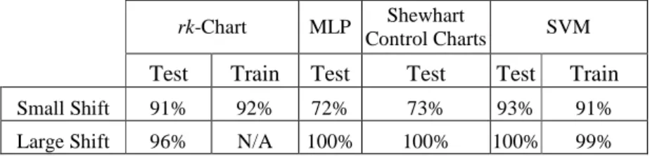
Table 6: Classification Accuracy ofrk-Chart versus MLP, Shewhart Charts and SVM charts using the
benchmarking dataset from Smith (1994). *in: In-control data, out: Out-of-control data.
rk-Chart MLP Shewhart
Control Charts SVM
Test Train Test Test Test Train
Small Shift 91% 92% 72% 73% 93% 91%
In the first category, classification accuracy is reported in methods such as MLP, Shewhart chart and SVM instead of Type-I and Type-II errors. Thus, the classification accuracy ofrk-Chart is calculated in order to compare the results with these methods. The weighted average of Type-I and Type-II errors are calculated, considering the number of patterns used for in-control and out-of-control data. As seen from Table 6, rk-Chart performs better than MLP and Shewhart charts. SVM is only 1% to 4% better thanrk-Chart. Even though SVM method gives better results than rk-Chart, there are two difficulties of implementing SVM and MLP in real world settings:
1. A distinct model is developed for each of the out-of-control state for SVM and MLP. There are four out-of-control states (SM, LM, SV, LV) resulting in four SVM and MLP models. Even though each model works well for developed out-of-control states, they cannot effectively work for other out-of-control states that are yet to have a model. In addition, SVM and MLP may be sensitive to an undefined out-of-control state. In contrast,rk-Chart characterizes the in-control state of the process and it has the ability to detect any undefined and unseen type of out-of-control state.
2. SVM and MLP are trained with 300 samples from in-control state and 300 samples from each modeled out-of-control state resulting in 4 models using a total of 2400 samples. On the other hand, rk-Chart uses only 300 samples from in-control state and 200 samples from out-of-control states.
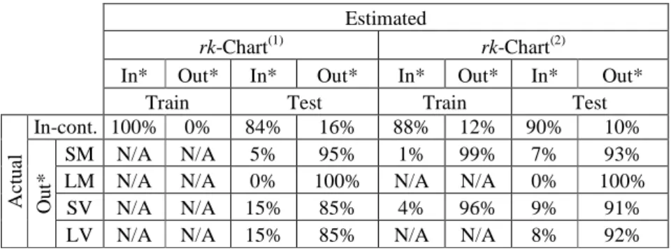
Table 7: Type-I and Type-II errors for the benchmarking dataset from Smith (1994) usingrk-Chart.
In*: in-control state, Out*: Out-of-control state.rk-Chart(1): Training with 300 normal samples.rk-Chart(2):
Training with 300 normal and 200 abnormal samples (100 small mean shift, 100 small variance shift) Estimated
rk-Chart(1) rk-Chart(2)
In* Out* In* Out* In* Out* In* Out*
Train Test Train Test
A c tu a l In-cont. 100% 0% 84% 16% 88% 12% 90% 10% O u t* SM N/A N/A 5% 95% 1% 99% 7% 93%
LM N/A N/A 0% 100% N/A N/A 0% 100%
SV N/A N/A 15% 85% 4% 96% 9% 91%
In the second category, we will report rk-Chart results with no and limited out-of-control data. In the former case (i.e.rk-Chart(1)), only 300 samples of in-control data are used for training, in the latter case (i.e. rk-Chart(2)) 300 samples of in-control and 100 samples of small mean shift and 100 samples of small variance shift are employed for training. The Type-I and Type-II errors as given in Table 7 are promising with 16% Type-I error and highest 15% Type-II error in rk-Chart(1)and 12% Type-I error and highest 9% Type-II error withrk-Chart(2).
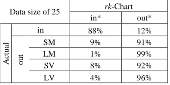
In the third category, rk-Chart is implemented with very limited in-control data. We implemented rk-Chart with 25 training patterns from the benchmarking Smith (Smith 1994) dataset and results are shown in Table 8.
Table 8: Process state classification for non-correlated Smith data with limited number of in-control and out-of-control samples (i. e. 25 in-control and 10 out-of-control patterns)
Data size of 25 rk-Chart
in* out* A c tu a l in 88% 12% o u t SM 9% 91% LM 1% 99% SV 8% 92% LV 4% 96%
As seen from Table 8, in the worst of the cases tested,rk-Chart had the power to effectively detect out-of-control conditions 91% of the time (9% Type-II error), with false alarm rate of only 12% (Type-I error) even with limited data size.
As for parameter selection in initializingrk-Charts, when the control chart is initialized with just control data, two parameters are required: a penalty value for misclassification of in-control data (C) and compactness (). The recommended default parameter values are 1.0 and 0.2, for Cand , respectively. An additional penalty parameter (C0) is required for cases with any available out-of-control data for initialization. The recommended default parameter value is once again 1.0. All the experimental results reported here are based on these default settings. Extensive experimentation with these parameters suggests that the rk-Chart is relatively robust
with respect to parameter value selection and that the recommended default values work well in most cases. However, individual applications can call for different types of tradeoffs between Type-I and Type-II errors, which call for appropriate selection or tuning ofrk-Chart parameters.
V. CONCLUSION
A new process control technique based on support vector machine principles, called robust kernel-distance control chart (rk-Chart), is proposed for both univariate and multivariate processes. rk-Chart has several advantages over the conventional SPC techniques and pattern recognition methods in the literature. rk-Chart does not make any assumption about the data distribution, which is a fundamental restriction for conventional SPC techniques. In addition, conventional SPC techniques cannot benefit from available out-of-control data, whereasrk-Chart can learn from out-of-control samples, where applicable. Pattern recognition methods used for process control in the literature based on other support vector machine (SVM) principles, radial-basis function (RBF) networks, and multi-layer-perceptron (MLP) neural networks require excessive amount of in-control data as well as out-of-control data. Furthermore, a distinct model for each type of out-of-control process needs to be created and trained using both in-control and out-of-control data with SVM, RBF and MLP. These models are not sensitive to out-of-control conditions other than those on which they are trained. In contrary, rk-Chart characterizes in-control-processes and requires only in-control data. However, it makes an explicit provision to accommodate any available out-of-control data. Thus, it is sensitive to all types of out-of-control processes. It is also shown that rk-Chart is able to give very reasonable results with limited in-control and out-of-in-control data when tested using a variety of datasets.
ACKNOWLEDGEMENTS
REFERENCES
Aradhye, H. B., Bakshi, B. R., Strauss, R. A. and Davis, J. F. (2001). Multiscale
statistical process control using wavelets: Theoretical analysis and properties. Columbus, OH, Ohio State University.
Bakshi, B., Multiscale PCA with application to multivariate statistical process
monitoring.Journal of the American Institute of Chemical Engineers, 1998,44, 1596-1610.
Chakraborti, S., Van der Laan, P. and Bakir, S. T., Nonparametric control charts: An overview and some results.Journal of Quality Technology, 2001,33, 304-315. Chakraborti, S., Van der Laan, P. and Van de Wiel, M., A class of distribution-free control charts.Journal of the Royal Statistical Society, Series C, 2004, 55(3), 443-462 Chen, Q., Kruger, U., Meronk, M. and Leung, A. Y. T., Synthetic of t2 and q statistics for process monitoring, control engineering practice.Control Engineering Practice, 2004,
12, 745-755.
Chinnam, R. B., Support vector machines for recognizing shifts in correlated and other manufacturing processes.International Journal of Production Research, 2002,40, 4449-4466.
Chinnam, R. B. and Kolarik, W. J., Automation and the total quality paradigm, in
Proceedings of the 1st IERC, 1992, Chicago, IL, IIE.
Cook, D. F. and Chiu, C., Using radial basis function neural networks to recognize shifts in correlated manufacturing process parameters.IIE Transactions, 1998,30, 227-234. Cristianini, N. and Taylor, J. S.,An introduction to support vector machines and other
kernel-based learning methods. (Cambridge: Cambridge University Press).
Eickelmann, N. and Anant, A., Statistical process control: What you don't measure can hurt you!Software, IEEE, 2003,20, 49-51.
Hotelling, H. (1947). Multivariate quality control-illustrated by the air testing of sample bombsights. Techniques of statistical analysis. C. Eisenhart, M. W. Hastay and W. A. Wallis. New York, McGraw-Hill:111-184.
Kuhn, H. and Tucker, A., Nonlinear programming, inProceedings of 2nd Berkeley
Symposium on Mathematical Statistics and Probabilistics, 1951, Berkely, CA, University
of California Press, 481-492.
Liu, R. Y. and Singh, K., A quality index based on data depth and multivariate rank tests.
Lowry, C. A. and Montgomery, D. C., A review of multivariate control charts.IIE
Transactions, 1995,27, 800-810.
Lowry, C. A., Woodall, W. H., Champ, C. W. and Rigdon, S. E., A multivariate exponentially weighted moving average control chart.Technometrics, 1992,34, 46-53. MacGregor, J. F. and Kourti, T., Statistical process control of multivariate processes.
Control Engineering Practice, 1995,3, 403-414.
Manabu, K., Shinji, H., Iori, H. and Hiromu, O., Evolution of multivariate statistical process control: Application of independent component analysis and external analysis.
Computers & Chemical Engineering, 2004,28, 1157-1166.
Mangasarian, O. L.,Nonlinear programming. (Philadelphia, PA: Society for Industrial and Applied Mathematics).
Martin, E. B., Morris, A. J. and Zhang, J., Process performance monitoring using multivariate statistical process control.IEE Proceedings, 1996,143, 132-144.
Mercer, J., Functions of positive and negative type and their connection with the theory of integral equations.Philosophical Transactions of the Royal Society of London, Series A, 1909,209, 415-446.
Messaoud, A., Weihs, C. and Hering, F. (2004). A nonparametric multivariate control chart based on data depth. Dortmund, Germany, Department of Statistics, University of Dortmund.
Montgomery, D. C.,Introduction to statistical quality control. (New York: Wiley). Müller, K. R., Mika, S., Rätsch, G., Tsuda, K. and Schölkopf, B., An introduction to kernel-based learning algorithms.IEEE Neural Networks, 2001,12, 181-201.
Ngai, H. and Zhang, J., Multivariate cumulative sum control charts based on projection pursuit.Statistica Sinica, 2001,11, 747-766.
Nimmo, I., Adequately address abnormal situation operations.Chemical Engineering
Progress, 1995,91, 36-45.
Polansky, A. M., A smooth nonparametric approach to multivariate process capability.
Technometrics, 2001,43, 199-211.
Pugh, G. A., A comparison of neural networks to spc charts. Computers and Industrial
Raich, A. and Cinar, A., Statistical process monitoring and disturbance diagnosis in multivariate continuous processes.Journal of the American Institute of Chemical
Engineers, 1996,42, 995-1009.
Rose, K., Mathematics of success and failure.Circuits and Devices, IEEE, 1991,7, 26-30.
Runger, G. C. and Prabhu, S. S., A markov chain model for the multivariate exponentially weighted moving averages control chart.Journal of the American
Statistical Association (JASA), 1996,91, 1701-1706.
Runger, G. C. and Testik, M. C., Multivariate extensions to cumulative sum control charts.Quality and Reliability Engineering International, 2004,20, 587 - 606.
Schilling, E. G. and Nelson, P.R., The effect of non-normality on the control limits of X
charts.Journal of Quality Technology, 1976,8, 183-187.
Shewhart, W. A., Quality control charts.Bell System Technical Journal, 1926,22, 593-603.
Smith, A. E., X-bar and r control chart interpretation using neural computing.
International Journal of Production Research, 1994,32, 309-320.
Stoumbos, Z. G. and Reynolds, M. R., On shewhart-type nonparametric multivariate control charts based on data depth.Frontiers in Statistical Quality Control, 2001,6, 207-227.
Sun, R. and Tsung, F., A kernel-distance-based multivariate control chart using support vector methods.International Journal of Production Research, 2003,41, 2975-2989. Tax, D. M. (2001). One class classification. Delft, The Netherlands, Delft Technical University.
Tax, D. M. J. and Duin, R. P. W., Support vector domain description.Pattern
Recognition Letters, 1999,20, 1191-1199.
Tax, D. M. J. and Duin, R. P. W., Support vector data description.Machine Learning, 2004,54, 45-66.
Teppola, P. and Minkkinen, P., Wavelet-pls regression models for both exploratory data analysis and process monitoring.Journal of Chemometrics, 2000,14, 383-399.
Testik, M. C. and Borror, C. M., Design strategies for the multivariate exponentially weighted moving average control chart.Quality and Reliability Engineering
Vapnik, V.,Statistical learning theory. (New York: Wiley).
Woodall, W. H. and Montgomery, D. C., Research issues and ideas in statistical process control.Journal of Quality Technology, 1999,31, 376-386.
Yoon, S. and MacGregor, J. F., Principal-component analysis of multiscale data for process monitoring and fault diagnosis.Journal of the American Institute of Chemical
Engineers, 2004,50, 2891-2903.
Yuan, C. and Casasent, D., Support vector machines for class representation and discrimination, inInternational Joint Conference on Neural Networks, 2003, Portland, OR, 1610-1615.