Lower bounds for Howard’s algorithm for
finding Minimum Mean-Cost Cycles
Thomas Dueholm Hansen1? and Uri Zwick2 1 Department of Computer Science, Aarhus University. 2
School of Computer Science, Tel Aviv University, Tel Aviv 69978, Israel.
Abstract. Howard’s policy iteration algorithm is one of the most widely used algorithms for finding optimal policies for controllingMarkov De-cision Processes (MDPs). When applied to weighted directed graphs, which may be viewed asDeterministicMDPs (DMDPs), Howard’s algo-rithm can be used to find Minimum Mean-Cost cycles (MMCC). Exper-imental studies suggest that Howard’s algorithm works extremely well in this context. The theoretical complexity of Howard’s algorithm for finding MMCCs is a mystery. No polynomial time bound is known on its running time. Prior to this work, there were only linear lower bounds on the number of iterations performed by Howard’s algorithm. We provide the first weighted graphs on which Howard’s algorithm performsΩ(n2)
iterations, wherenis the number of vertices in the graph.
1
Introduction
Howard’s policy iteration algorithm [11] is one of the most widely used algorithms for solving Markov decision processes (MDPs). The complexity of Howard’s algo-rithm in this setting was unresolved for almost 50 years. Very recently, Fearnley [5], building on results of Friedmann [7], showed that there are MDPs on which Howard’s algorithm requires exponential time. In another recent breakthrough, Ye [17] showed that Howard’s algorithm is strongly polynomial when applied to discounted MDPs, with a fixed discount ratio. Hansen et al. [10] recently improved some of the bounds of Ye and extended them to the 2-player case.
Weighted directed graphs may be viewed asDeterministic MDPs (DMDPs) and solving such DMDPs is essentially equivalent to finding minimum mean-cost cycles (MMCCs) in such graphs. Howard’s algorithm can thus be used to solve this purely combinatorial problem. The complexity of Howard’s algorithm in this setting is an intriguing open problem. Fearnley’s [5] exponential lower bound seems to depend in an essential way on the use of stochastic actions, so it does not extend to the deterministic setting. Similarly, Ye’s [17] polynomial upper bound depends in an essential way on the MDPs being discounted and does not extend to the non-discounted case.
?
Supported by the Center for Algorithmic Game Theory at Aarhus University, funded by the Carlsberg Foundation.
The MMCC problem is an interesting problem that has various applications. It generalizes the problem of finding a negative cost cycle in a graph. It is also used as a subroutine in algorithms for solving other problems, such as min-cost flow algorithms, (See, e.g., Goldberg and Tarjan [9].)
There are several polynomial time algorithms for solving the MMCC problem. Karp [12] gave anO(mn)-time algorithm for the problem, wheremis the number of edges and n is the number of vertices in the input graph. Younget al. [18] gave an algorithm whose complexity isO(mn+n2logn). Although this is slightly worse, in some cases, than the running time of Karp’s algorithm, the algorithm of Younget al.[18] behaves much better in practice.
Dasdan [3] experimented with many different algorithms for the MMCC prob-lem, including Howard’s algorithm. He reports that Howard’s algorithm usually runs much faster than Karp’s algorithm, and is usually almost as fast as the algorithm of Younget al. [18]. A more thorough experimental study of MMCC algorithms was recently conducted by Georgiadiset al.[8].3
Understanding the complexity of Howard’s algorithm for MMCCs is interest-ing from both the applied and theoretical points of view. Howard’s algorithm for MMCC is an extremely simple and natural combinatorial algorithm, similar in flavor to the Bellman-Ford algorithm for finding shortest paths [1, 2],[6] and to Karp’s [12] algorithm. Yet, its analysis seems to be elusive. Howard’s algorithm also has the advantage that it can be applied to the more general problem of finding a cycle with aminimum cost-to-time ratio (see, e.g., Megiddo [14, 15]).
Howard’s algorithm works in iteration. Each iteration takesO(m) time. It is trivial to construct instances on which Howard’s algorithm performsniterations. (Recall thatnandmare the number of vertices and edges in the input graph.) Madani [13] constructed instances on which the algorithm performs 2n−O(1) iterations. No graphs were known, however, on which Howard’s algorithm per-formed more than alinear number of iterations. We construct the first graphs on which Howard’s algorithm performsΩ(n2) iterations, showing, in particular, that there are instances on which its running time is Ω(n4), an order of magni-tudeslower than the running times of the algorithms of Karp [12] and Younget al. [18].
We also constructn-vertex outdegree-2 graphs on which Howard’s algorithm performs 2n−O(1) iterations. (Madani’s [13] examples usedΘ(n2) edges.) This example is interesting as it shows that the number of iterations performed may differ from the number of edges in the graph by only an additive constant. It also sheds some more light on the non-trivial, and perhaps non-intuitive behavior of Howard’s algorithm.
Our examples still leave open the possibility that the number of iterations performed by Howard’s algorithm is always at most m, the number of edges. (The graphs on which the algorithm performsΩ(n2) iterations also haveΩ(n2) edges.) We conjecture that this is always the case.
3 Georgiadis et al. [8] claim that Howard’s algorithm is not robust. From personal
conversations with the authors of [8] it turns out, however, that the version they used is substantially different from Howard’s algorithm [11].
2
Howard’s algorithm for minimum mean-cost cycles
We next describe the specialization of Howard’s algorithm for deterministic
MDPs, i.e., for finding Minimum Mean-Cost Cycles. For Howard’s algorithm for general MDPs, see Howard [11], Derman [4] or Puterman [16].
LetG= (V, E, c), wherec:E→R, be a weighted directed graph. We assume
that each vertex has a unique serial number associated with. We also assume, without loss of generality, that each vertexv∈V has at least one outgoing edge. If C =v0v1. . . vk−1v0 is a cycle in G, we let val(C) = k1Pik=0−1c(vi, vi+1), wherevk =v0, be itsmean cost. The vertex onCwith the smallest serial number is said to be thehead of the cycle. Our goal is to find a cycleC that minimizes
val(C).
Apolicy πis a mappingπ:V →V such that (v, π(v))∈E, for everyv∈V. A policyπ, defines a subgraph Gπ = (V, Eπ), whereEπ ={(v, π(v))|v ∈V}.
As the outdegree of each vertex in Gπ is 1, we get that Gπ is composed of a
collection of disjoint directed cycles with directed paths leading into them. Given a policy π, we assign to each vertex v0 ∈ V a value valπ(v0) and a potential potπ(v0) in the following way. Let Pπ(v0) = v0v1, . . . be the infinite path defined byvi=π(vi−1), fori >0. This infinite path is composed of a finite pathPleading to a cycleCwhich is repeated indefinitely. Ifvr=vr+kis the first
vertex visited for the second time, thenP =v0v1. . . vr andC=vrvr+1. . . vr+k.
We letv`be the head of the cycle C. We now define
valπ(v0) = val(C) = k1Pki=0−1c(vr+i, vr+i+1),
potπ(v0) = P`i=0−1(c(vi, vi+1)−val(C)).
In other words, valπ(v0) is the mean cost of C, the cycle into which Pπ(v0) is absorbed, while potπ(v0) is the distance from v0 to v`, the head of this cycle,
when the mean cost of the cycle is subtracted from the cost of each edge. It is easy to check that values and potentials satisfy the following equations:
valπ(v) = valπ(π(v)),
potπ(v) = c(v, π(v))−valπ(v) +potπ(π(v)).
Theappraisal of an edge (u, v)∈E is defined as the pair:
Aπ(u, v) = (valπ(v), c(u, v)−valπ(v) +potπ(v) ).
Howard’s algorithm starts with an arbitrary policy π and keeps improving
it. Ifπis the current policy, then the next policy π0 produced by the algorithm is defined by
π0(u) = arg min
v:(u,v)∈E
Aπ(u, v).
In other words, for every vertex the algorithm selects the outgoing edge with the lowest appraisal. (In case of ties, the algorithm favors edges in the current policy.) As appraisals are pairs, they are compared lexicographically, i.e., (u, v1) is better
than (u, v2) if and only ifAπ(u, v1)≺Aπ(u, v2), where (x1, y1)≺(x2, y2) if and only if x1 < x2, orx1 =x2 and y1 < y2. When π0 = π, the algorithm stops. The correctness of the algorithm follows from the following two lemmas whose proofs can be found in Howard [11], Derman [4] and Puterman [16].
Lemma 1. Suppose that π0 is obtained from π by a policy improvement step.
Then, for every v ∈ V we have (valπ0(v), potπ0(v)) (valπ(v), potπ(v)).
Fur-thermore, if π0(v)6=π(v), then(val
π0(v), potπ0(v))≺(valπ(v), potπ(v)).
Lemma 2. If policyπ is not modified by an improvement step, thenvalπ(v)is
the minimum mean weight of a cycle reachable from v in G. Furthermore by following edges ofπfrom v we get into a cycle of this minimum mean weight.
Each iteration of Howard’s algorithm takes onlyO(m) time and is not much more complicated than an iteration of the Bellman-Ford algorithm.
3
A quadratic lower bound
We next construct a family of weighted directed graphs for which the number of iterations performed by Howard’s algorithm is quadratic in the number of vertices. More precisely, we prove the following theorem:
Theorem 1. Let n and m be even integers, with 2n ≤ m ≤ n2
4 + 3n
2. There
exists a weighted directed graph withnvertices andm edges on which Howard’s algorithm performsm−n+ 1 iterations.
All policies generated by Howard’s algorithm, when run on the instances of Theorem 1, contain a single cycle, and hence all vertices have the same value. Edges are therefore selected for inclusion in the improved policies based on poten-tials. (Recall that potentials are essentially adjusted distances.) The main idea behind our construction, which we refer to as the dancing cycles construction, is the use of cycles of very large costs, so that Howard’s algorithm favors long, i.e., containing many edges, paths to the cycle of the current policy attractive, delaying the discovery of better cycles.
Given a graph and a sequence of policies, it is possible check, by solving an appropriate linear program, whether there exist costs for which Howard’s algorithm generates the given sequence of policies. Experiments with a program that implements this idea helped us obtain the construction presented below.
For simplicity, we first prove Theorem 1 for m = n42 + 32n. We later note that the same construction works when removing pairs of edges, which gives the statement of the theorem.
3.1 The Construction
For everynwe construct a weighted directed graphGn= (V, E, c), on|V|= 2n
vertices and |E| =n2+ 3n edges, and an initial policy π
0 such that Howard’s algorithm performsn2+n+ 1 iterations onG
The graphGn itself is fairly simple. (See Figure 1.) Most of the intricacy
goes into the definition of the cost function c : E → R. The graph Gn is
composed of two symmetric parts. To highlight the symmetry we let V =
{v0
n, . . . , v10, v11, . . . , vn1}. Note that the set of vertices is split in two, according
to whether the superscript is 0 or 1. In order to simplify notation when dealing with vertices with different superscripts, we sometimes refer tov0
1 as v10 and to
v1
1 asv00. The set of edges is:
E={(v0i, v0j),(v1i, v1j)|1≤i≤n, i−1≤j≤n}.
We next describe a sequence of policiesΠnof lengthn2+n+1. We then construct
a cost function that causes Howard’s algorithm to generate this long sequence of policies. For 1≤`≤r≤nands∈ {0,1}, and for`= 1,r= 0 ands= 0, we define a policyπs `,r: πs`,r(vit) = vt i−1 fort6=sori > ` vt r fort=sandi=` vt n fort=sandi < ` The policyπs
`,r contains a single cyclevrsvrs−1. . . vs`vsrwhich is determined by its
defining edgees
`,r= (vs`, vsr). As shown in Figure 1, all vertices to the left ofvs`,
thehead of the cycle, choose an edge leading furthest to the right, while all the vertices to the right ofvs
` choose an edge leading furthest to the left.
The sequenceΠn is composed of the policies π`,rs , where 1≤`≤r≤nand
s∈ {0,1}, or`= 1, r= 0 and s= 0, with the following ordering. Policyπs1
`1,r1
precedes policy πs2
`2,r2 in Πn if and only if `1 > `2, or `1 =`2 and r1 > r2, or `1 =`2 and r1 =r2 and s1 < s2. (Note that this is a reversed lexicographical ordering on the triplets (`1, r1,1−s1) and (`2, r2,1−s2).) For every 1≤`≤r≤n and s∈ {0,1}, or `= 1, r = 0 ands= 0, we let f(`, r, s) be the index ofπs
`,r
in Πn, where indices start at 0. We can now write:
Πn= (πk)n 2+n k=0 = πns−`,n−r 1 s=0 ` r=0 n−1 `=0 , π10,0
We refer to Figure 1 for an illustration ofG4and the corresponding sequenceΠ4.
3.2 The edge costs
Recall that each policyπk =πs`,r is determined by an edge ek=es`,r = (v`s, vrs),
where k =f(`, r, s). LetN =n2+n. We assign the edges the following
expo-nential costs: c(ek) = c(v`s, vrs) = nN−k , 0≤k < N, c(v0 1, v11) = c(v11, v01) = −nN , c(vs i, vis−1) = 0 , 2≤i≤n , s∈ {0,1}.
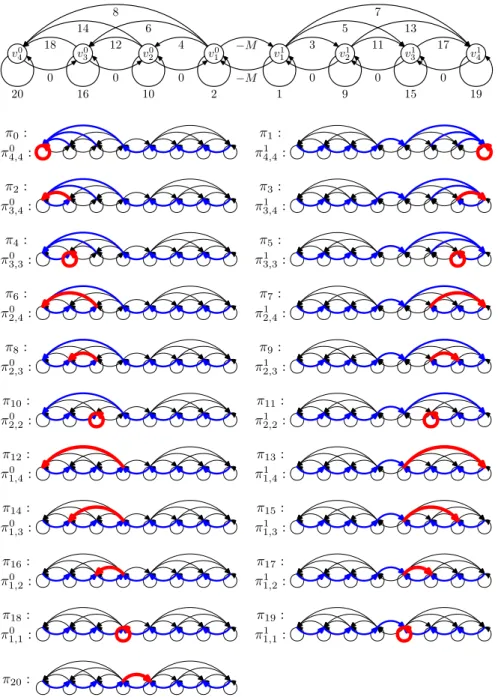
π0 4,4: π0: π1 4,4: π1: π0 3,4: π2: π1 3,4: π3: π0 3,3: π4: π1 3,3: π5: π0 2,4: π6: π1 2,4: π7: π0 2,3: π8: π1 2,3: π9: π0 2,2: π10: π1 2,2: π11: π0 1,4: π12: π1 1,4: π13: π0 1,3: π14: π1 1,3: π15: π0 1,2: π16: π1 1,2: π17: π0 1,1: π18: π1 1,1: π19: π20: v0 4 v03 v20 v01 v11 v21 v13 v14 20 0 18 16 0 14 12 10 0 8 6 4 2 −M 7 5 3 1 −M 13 11 9 0 17 15 0 19 0
Fig. 1. G4 and the corresponding sequence Π4. Π4 is shown in left-to-right order. Policiesπf(`,r,s)=πs`,rare shown in bold, withes`,r being highlighted. Numbers below edges define costs. 0 means 0,k >0 meansnk, and−M means−nN.
We claim that with these exponential edge costs Howard’s algorithm does indeed produce the sequenceΠn. To show thatπk+1is indeed the policy that Howard’s algorithm obtains by improvingπk, we have to show that
πk+1(u) = arg min
v:(u,v)∈E
Aπk(u, v) , ∀u∈V. (1)
For brevity, we let c(vs
i, vsj) = csi,j. The only cycle in πk = π`,rs is C`,rs =
vs
rvsr−1. . . v`svrs. Asci,is −1= 0, for 2≤i≤nands∈ {0,1}, we have
µs `,r = val(C`,rs ) = cs `,r r−`+ 1. Ascs
`,r=nN−k and all cycles in our construction are of size at mostnwe have
nN−k−1 ≤ µs`,r ≤ nN−k.
As all vertices have the same value µs
`,r under πk = π`,rs , edges are compared
based on the second component of their appraisalsAπk(u, v). Hence, (1) becomes: πk+1(u) = arg min
v:(u,v)∈E
c(u, v) +potπk(v) , ∀u∈V. (2)
Note that an edge (u, v1) is preferred over (u, v2) if and only if
c(u, v1)−c(u, v2)< potπk(v2)−potπk(v1).
Letvs
` be the head of the cycle C`,rs . Keeping in mind thatcsi,i−1 = 0, for 2 ≤ i ≤ n and s ∈ {0,1}, it is not difficult to see that the potentials of the vertices under policy πs
`,r are given by the following expression:
potπs `,r(v t i) = cs i,n−(n−`+ 1)µs`,r ift=sandi < `, −(i−`)µs `,r ift=sandi≥`, ct 1,0−iµs`,r+potπs `,r(v s 1) if t6=s. It is convenient to note that we havepotπs
`,r(v t
i)≤0, for every 1≤`≤r≤n,
1≤i≤nand s, t∈ {0,1}. In the first case (t=sand i < `), this follows from the fact that (vs
i, vsn) has a larger index than (v`s, vsr) (note thati < `). In the
third case (t=s), it follows from the fact thatct
1,0=−nN <0.
3.3 The dynamics
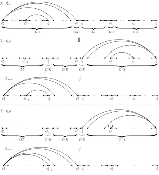
The proof that Howard’s algorithm produces the sequence Πn is composed of
three main cases, shown in Figure 2. Each case is broken into several subcases. Each subcase on its own is fairly simple and intuitive.
Case 1. Suppose thatπk =π0`,r. We need to show thatπk+1 =π`,r1 . We have
v0 n . . . v0 r . . . v0 ℓ . . . v0 1 vn1 . . . v1 r . . . v1 ℓ . . . v1 1
{
(1.1) (1.2){
(1.3){
(1.4){
(1.5){
(1) π0 ℓ,r: v0 n . . . v0 r−1 . . . v0 ℓ . . . v0 1 vn1 . . . v1 r . . . v1 ℓ . . . v1 1{
(2.5) (2.4){
(2.3){
(2.2){
(2.1){
(2) π1 ℓ,r:⇒
v0 n . . . v0 r−1 . . . v0 ℓ . . . v0 1 v1n . . . v1 r . . . v1 ℓ . . . v1 1 π0 ℓ,r−1:⇒
v0 n . . . v0 ℓ−1 . . . v0 1 v1n . . . v1 ℓ . . . v1 1{
(3.5) (3.4){
(3.3){
(3.2){
(3.1){
(3) π1 ℓ,ℓ: v0 n . . . v0 ℓ−1 . . . v0 1 v1n . . . v1 ℓ . . . v1 1 π0 ℓ−1,n:⇒
Fig. 2.Policies of transitions (1)π0`,r toπ
1 `,r, (2)π 1 `,r toπ 0 `,r−1, and (3)π 1 `,`toπ 0 `−1,n. Vertices of the corresponding subcases have been annotated accordingly.
Case 1.1.We show thatπk+1(vi0) =v0i−1, for 2≤i≤n. We have to show that (v0
i, vi0−1) beats (vi0, vj0), for every 2≤i≤j≤n, or in other words that
c0 i,i−1+potπ0 `,r(v 0 i−1) < c0i,j+potπ0 `,r(v 0 j) , 2≤i≤j≤n.
Case 1.1.1.Assume thatj < `. We then have
potπ0 `,r(v 0 i−1) = c0i−1,n−(n−`+ 1)µ0`,r, potπ0 `,r(v 0 j) = c0j,n−(n−`+ 1)µ0`,r.
Recalling thatc0
i,i−1= 0, the inequality that we have to show becomes
c0
i−1,n < c0i,j+c0j,n , 2≤i≤j < `≤n.
As the edge (v0
i−1, vn0) comesafter (vi0, vj0) in our ordering, we havec0i−1,n< c0i,j.
The other term on the right is non-negative and the inequality follows easily.
Case 1.1.2.Assume thati−1< `≤j. We then have
potπ0 `,r(v 0 i−1) = c0i−1,n−(n−`+ 1)µ0`,r, potπ0 `,r(v 0 j) = −(j−`)µ0`,r,
and the required inequality becomes
c0i−1,n < c0i,j+ (n−j+ 1)µ0`,r , 1≤i−1< `≤j≤n.
Asj≤n, the inequality again follows from the fact thatc0
i−1,n< c0i,j.
Case 1.1.3.Assume that`≤i−1< j. We then have
potπ0 `,r(v 0 j)−potπ0 `,r(v 0 i−1) = (i−j−1)µ0`,r,
and the required inequality becomes (j−i+ 1)µ0
`,r < c0i,j , 1≤`≤i−1< j≤n.
This inequality holds as (j−i+ 1)µ0
`,r< n c0`,r≤c0i,j. The last inequality follows
as (v0
`, vr0) appears after (vi0, vj0) in our ordering. (Note that we are using here,
for the first time, the fact that the weights are exponential.)
Case 1.2.We show thatπk+1(v10) =v11. We have to show that
c0 1,0+potπ0 `,r(v 1 1) < c01,j+potπ0 `,r(v 0 j) , 1≤j≤n.
This inequality is easy. Note that c0
1,0 = −nN, potπ 0 `,r(v1 1) ≤0, while c01,j >0 andpotπ0 `,r(v 0 j)>−nN.
Case 1.3.We show thatπk+1(vi1) =vn1, for 1≤i < `. We have to show that
c1i,n−c1i,j < potπ0 `,r(v 1 j)−potπ0 `,r(v 1 n) , 1≤i < ` , i−1≤j < n.
Case 1.3.1.Suppose thati= 1 andj= 0. We need to verify that
c11,n−c11,0 < potπ0 `,r(v 1 0)−potπ0 `,r(v 1 n). Aspotπ0 `,r(v 1 0) =potπ0 `,r(v 0 1) andpotπ0 `,r(v 1 n) =c11,0−nµ0`,r+potπ0 `,r(v 0 1), we have to verify that c1
1,n < nµ0`,r, which follows from the fact that` > 1 and that
(v0
`, vr0) has a smaller index than (v11, v1n).
Case 1.3.2.Suppose thatj ≥1. We have to verify that
c1i,n−c1i,j < potπ0 `,r(v 1 j)−potπ0 `,r(v 1 n) = (n−j)µ`,r0 , 1≤i < ` , i−1≤j < n.
As in Case 1.3.1 we have c1
i,n≤µ0`,r whilec1i,j>0.
Case 1.4.We show thatπk+1(v`1) =vr1. We have to show that
c1`,r−c1`,j < potπ0 `,r(v 1 j)−potπ0 `,r(v 1 r) , `−1≤j ≤n , j6=r.
Case 1.4.1. Suppose that ` = 1 and j = 0. As in case 1.3.1, the inequality
becomes c11,r< rµ0`,r which is easily seen to hold.
Case 1.4.2.Suppose that`−1≤j < rand 0< j. We need to show that
c1 `,r−c1`,j < potπ0 `,r(v 1 j)−potπ0 `,r(v 1 r) = (r−j)µ0`,r , `−1≤j≤n , 0< j < r. As (v1
`, v1r) immediately follows (v`0, vr0) in our ordering, we havec1`,r =n−1c0`,r.
Thusc1
`,r ≤µ0`,r≤(r−j)µ0`,r. Asc1`,j >0, the inequality follows.
Case 1.4.3.Suppose thatr < j. We need to show that
c1`,r−c1`,j < potπ0 `,r(v 1 j)−potπ0 `,r(v 1 r) = (r−j)µ0`,r , r < j≤n,
or equivalently that c1`,j−c1`,r < (j−r)µ0`,r, for r < j≤n,. This follows from
the fact that (v1
`, v1r) comes after (v`1, v1j) in the ordering and thatc1`,r>0.
Case 1.5.We show thatπk+1(vi1) =vi1−1, for` < i≤n. We have to show that
c1i,i−1−c1i,j < potπs `,r(v 1 j)−potπs `,r(v 1 i−1) = (i−j−1)µs`,r , ` < i≤j≤n.
This is identical to case 1.1.3.
Case 2.Suppose thatπk=π1`,rand` < r. We need to show thatπk+1=π`,r0 −1. The proof is very similar to Case 1 and is omitted.
Case 3. Suppose that πk = π1`,`. We need to show that πk+1 = π0`−1,n. The
proof is very similar to Cases 1 and 2 and is omitted.
3.4 Remarks
For any 0 ≤ ` ≤ r < n, if the edges (v0
`, vr0) and (v1`, v1r) are removed from
Gn, then Howard’s algorithm skipsπ0`,r andπ`,r1 , but otherwiseΠn remains the
same. This can be repeated any number of times, essentially without modifying the proof given in Section 3.3, thus giving us the statement of Theorem 1.
Let us also note that the costs presented here have been chosen to simplify the analysis. It is possible to define smaller costs, but assuming cs
i,i−1 = 0 for
s ∈ {0,1} and 2 ≤ i ≤ n, which can always be enforced using a potential transformation, any costs generatingΠn must satisfy the following subset of the
inequalities from cases 1.4.2 and 2.4.2:
c1 1,r−c11,r−1 < µ01,r= c0 1,r r , 2≤r≤n c0 1,r−1−c01,r−2 < µ11,r = c1 1,r r , 3≤r≤n .
{
S ta g e 1{
S ta g e 2{
S ta g e 3{
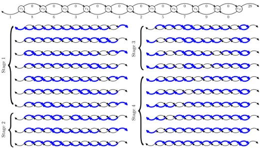
S ta g e 4 v1 v2 v3 v4 v5 v6 v7 v8 v9 v10 v11 1 0 8 0 6 0 3 0 1 0 4 0 2 0 5 0 7 0 9 0 0 28Fig. 3.G5 and the corresponding sequence of policies.
Letw2r−s=cs1,r. Joining the inequalities we get:
wk>
k
2
(wk−1−wk−3) , 4≤k≤2n .
It is then easy to see that for integral costs the size of the costs must be expo-nential inn.
4
A 2
n
−
O
(1) lower bounds for outdegree-2 graphs
In this section we briefly mention a construction of a sequence of outdegree-2 DMDPs on which the number of iterations of Howard’s algorithm is only two less than the total number of edges.
Theorem 2. For every n ≥ 3 there exists a weighted directed graph Gn =
(V, E, c), where c : E → R, with |V| = 2n+ 1 and |E| = 2|V|, on which
Howard’s algorithm performs |E| −2 = 4n iterations.
The graph used in the proof of Theorem 2 is simply a bidirected cycle on 2n+ 1 vertices. (The graphG5 is depicted at the top of Figure 3.) The proof of Theorem 2 can be found in Appendix A.
5
Concluding remarks
We presented a quadratic lower bound on the number of iterations performed by Howard’s algorithm for finding Minimum Mean-Cost Cycles (MMCCs). Our
lower bound is quadratic in the number of vertices, but is only linear in the number of edges. We conjecture that this is best possible:
ConjectureThe number of iterations performed by Howard’s algorithm, when
applied to a weighted directed graph, is at most the number of edgesin the graph.
Proving (or disproving) our conjecture is a major open problem. Our lower bounds shed some light on the non-trivial behavior of Howard’s algorithm, even on deterministic DMDPs, and expose some of the difficulties that need to be overcome to obtain non-trivial upper bounds on its complexity.
Our lower bounds on the complexity of Howard’s algorithm do not undermine the usefulness of Howard’s algorithm, as the instances used in our quadratic lower bound are very unlikely to appear in practice.
Acknowledgement
We would like to thank Omid Madani for sending us his example [13], and to Mike Paterson for helping us to obtain the results of Section 4. We would also like to thank Daniel Andersson, Peter Bro Miltersen, as well as Omid Madani and Mike Paterson, for helpful discussions on policy iteration algorithms.
References
1. R.E. Bellman. Dynamic programming. Princeton University Press, 1957.
2. R.E. Bellman. On a routing problem.Quarterly of Applied Mathematics, 16:87–90, 1958.
3. A. Dasdan. Experimental analysis of the fastest optimum cycle ratio and mean algorithms. ACM Trans. Des. Autom. Electron. Syst., 9(4):385–418, 2004. 4. C. Derman. Finite state Markov decision processes. Academic Press, 1972. 5. J. Fearnley. Exponential lower bounds for policy iteration. InProc. of 37th ICALP,
2010. Preliminaey version available at http://arxiv.org/abs/1003.3418v1.
6. L. R. Ford, Jr. and D. R. Fulkerson. Maximal flow through a network. Canadian Journal of Mathematics, 8:399–404, 1956.
7. O. Friedmann. An exponential lower bound for the parity game strategy improve-ment algorithm as we know it. InProc. of 24th LICS, pages 145–156, 2009. 8. L. Georgiadis, A.V. Goldberg, R.E. Tarjan, and R.F.F. Werneck. An experimental
study of minimum mean cycle algorithms. InProc. of 11th ALENEX, pages 1–13, 2009.
9. A.V. Goldberg and R.E. Tarjan. Finding minimum-cost circulations by canceling negative cycles. Journal of the ACM, 36(4):873–886, 1989.
10. T.D. Hansen, P.B. Miltersen, and U. Zwick. Strategy iteration is strongly poly-nomial for 2-player turn-based stochastic games with a constant discount factor.
CoRR, abs/1008.0530, 2010.
11. R.A. Howard. Dynamic programming and Markov processes. MIT Press, 1960. 12. R.M. Karp. A characterization of the minimum cycle mean in a digraph. Discrete
Mathematics, 23(3):309–311, 1978.
14. N. Megiddo. Combinatorial optimization with rational objective functions. Math-ematics of Operations Research, 4(4):414–424, 1979.
15. N. Megiddo. Applying parallel computation algorithms in the design of serial algorithms. Journal of the ACM, 30(4):852–865, 1983.
16. M.L. Puterman. Markov decision processes. Wiley, 1994.
17. Y. Ye. The simplex method is strongly polynomial for the Markov decision problem with a fixed discount rate. Available at http://www.stanford.edu/ yyye/simplexmdp1.pdf, 2010.
18. N.E. Young, R.E. Tarjan, and J.B. Orlin. Faster parametric shortest path and minimum-balance algorithms. Networks, 21:205–221, 1991.
APPENDIX
A
A 2
n
−
O
(1) lower bounds for outdegree-2 graphs
A.1 The construction
LetV ={v1, . . . , v2n+1}. We let v2n+2 =v1andv0=v2n+1. Let
E={(vi, vi−1),(vi, vi+1)|1≤i≤2n+ 1}.
The graph Gn is simply abidirected cycle on 2n+ 1 vertices. (The graphG5 is depicted at the top of Figure 3.) We define costs, forn≥3, as follows:
i 1 2≤i≤n−2n−1 n n+ 1n+ 2n+ 3≤i≤2n2n+ 1
c(vi, vi−1) 1 2(n−i+ 1) 3 1 4 2 2(i−n) + 1 0
i 1≤i≤2n 2n+ 1
c(vi, vi+1) 0 Pk2n=nc(vk, vk−1)
We describe a sequence of policiesΠn = (πj)4jn=1 of length 4ngenerated by running Howard’s algorithm onGn, starting withπ1. Let us first introduce some notation. We describe a policyπ as a sequence of indices [i1, . . . , ik], such that
for every 1≤j ≤2n+ 1, ifi`−1 ≤j < i` where ` is odd, then π(vj) = vj+1. Otherwise,π(vj) =vj−1. We always assume that i0= 1 and ik+1= 2n+ 2. In other words, for every j ∈ [i0, i1)∪[i2, i3)∪. . ., we have π(vj) = vj+1, while for every j ∈ [i1, i2)∪[i3, i4)∪. . ., we haveπ(vj) = vj−1 The sequenceΠn is
composed of four subsequencesΠ1
n, Πn2, Πn3, Πn4 that we callstages.
Πn1= [1,2n+ 1], [2n−k+ 1],[k+ 1,2n] n−2 k=1 Πn2= [n, n+ 1, n+ 2],[n,2n],[n] Πn3= [1, k+ 1, n,2n−k,2n+ 1] n−2 k=0 Π4 n= [1, n+ 2−k,2n+ 1] n+1 k=1 Thus, for example:
Πn1= [1,2n+ 1],[2n],[2,2n],[2n−1],[3,2n], . . . ,[n+ 3],[n−1,2n]
Doing a case analysis, similar to that of Section 3.3, it is possible to prove that the sequence Πn is indeed the sequence of policies generated by running
Howard’s algorithm on Gn, starting at [1,2n+ 1]. The proof can be found in
Appendix A.
For alternative pictorial description of the sequenceΠn, forn= 15, is given
APPENDIX 1 1 1 1 1 1 1 1 1 1 1 1 1 1 1 1 1 1 1 1 1 1 1 1 1 1 1 1 1 1 2 2 2 2 2 2 2 2 2 2 2 2 2 2 2 2 2 2 2 2 2 2 2 2 2 2 2 2 2 2 1 1 2 1 1 1 1 1 1 1 1 1 1 1 1 1 1 1 1 1 1 1 1 1 1 1 1 1 1 1 1 2 2 2 2 2 2 2 2 2 2 2 2 2 2 2 2 2 2 2 2 2 2 2 2 2 2 2 2 2 2 1 1 1 2 2 1 1 1 1 1 1 1 1 1 1 1 1 1 1 1 1 1 1 1 1 1 1 1 1 1 1 1 2 2 2 2 2 2 2 2 2 2 2 2 2 2 2 2 2 2 2 2 2 2 2 2 2 2 2 2 2 1 1 1 1 2 2 2 1 1 1 1 1 1 1 1 1 1 1 1 1 1 1 1 1 1 1 1 1 1 1 1 1 1 2 2 2 2 2 2 2 2 2 2 2 2 2 2 2 2 2 2 2 2 2 2 2 2 2 2 2 2 1 1 1 1 1 2 2 2 2 1 1 1 1 1 1 1 1 1 1 1 1 1 1 1 1 1 1 1 1 1 1 1 1 1 2 2 2 2 2 2 2 2 2 2 2 2 2 2 2 2 2 2 2 2 2 2 2 2 2 2 2 1 1 1 1 1 1 2 2 2 2 2 1 1 1 1 1 1 1 1 1 1 1 1 1 1 1 1 1 1 1 1 1 1 1 1 2 2 2 2 2 2 2 2 2 2 2 2 2 2 2 2 2 2 2 2 2 2 2 2 2 2 1 1 1 1 1 1 1 2 2 2 2 2 2 1 1 1 1 1 1 1 1 1 1 1 1 1 1 1 1 1 1 1 1 1 1 1 2 2 2 2 2 2 2 2 2 2 2 2 2 2 2 2 2 2 2 2 2 2 2 2 2 1 1 1 1 1 1 1 1 2 2 2 2 2 2 2 1 1 1 1 1 1 1 1 1 1 1 1 1 1 1 1 1 1 1 1 1 1 2 2 2 2 2 2 2 2 2 2 2 2 2 2 2 2 2 2 2 2 2 2 2 2 1 1 1 1 1 1 1 1 1 2 2 2 2 2 2 2 2 1 1 1 1 1 1 1 1 1 1 1 1 1 1 1 1 1 1 1 1 1 2 2 2 2 2 2 2 2 2 2 2 2 2 2 2 2 2 2 2 2 2 2 2 1 1 1 1 1 1 1 1 1 1 2 2 2 2 2 2 2 2 2 1 1 1 1 1 1 1 1 1 1 1 1 1 1 1 1 1 1 1 1 2 2 2 2 2 2 2 2 2 2 2 2 2 2 2 2 2 2 2 2 2 2 1 1 1 1 1 1 1 1 1 1 1 2 2 2 2 2 2 2 2 2 2 1 1 1 1 1 1 1 1 1 1 1 1 1 1 1 1 1 1 1 2 2 2 2 2 2 2 2 2 2 2 2 2 2 2 2 2 2 2 2 2 1 1 1 1 1 1 1 1 1 1 1 1 2 2 2 2 2 2 2 2 2 2 2 1 1 1 1 1 1 1 1 1 1 1 1 1 1 1 1 1 1 2 2 2 2 2 2 2 2 2 2 2 2 2 2 2 2 2 2 2 2 1 1 1 1 1 1 1 1 1 1 1 1 1 2 2 2 2 2 2 2 2 2 2 2 2 1 1 1 1 1 1 1 1 1 1 1 1 1 1 1 1 1 2 2 2 2 2 2 2 2 2 2 2 2 2 2 2 2 2 2 2 1 1 1 1 1 1 1 1 1 1 1 1 1 1 2 2 2 2 2 2 2 2 2 2 2 2 2 1 1 1 1 1 1 1 1 1 1 1 1 1 1 1 1 2 2 2 2 2 2 2 2 2 2 2 2 2 2 2 2 1 2 1 1 1 1 1 1 1 1 1 1 1 1 1 1 1 2 2 2 2 2 2 2 2 2 2 2 2 2 2 1 1 1 1 1 1 1 1 1 1 1 1 1 1 1 2 2 2 2 2 2 2 2 2 2 2 2 2 2 2 2 1 1 1 1 1 1 1 1 1 1 1 1 1 1 1 1 1 2 2 2 2 2 2 2 2 2 2 2 2 2 2 1 1 1 1 1 1 1 1 1 1 1 1 1 1 1 2 1 1 2 2 2 2 2 2 2 2 2 2 2 2 2 1 1 1 1 1 1 1 1 1 1 1 1 1 1 2 2 1 1 1 2 2 2 2 2 2 2 2 2 2 2 2 1 1 1 1 1 1 1 1 1 1 1 1 1 2 2 2 1 1 1 1 2 2 2 2 2 2 2 2 2 2 2 1 1 1 1 1 1 1 1 1 1 1 1 2 2 2 2 1 1 1 1 1 2 2 2 2 2 2 2 2 2 2 1 1 1 1 1 1 1 1 1 1 1 2 2 2 2 2 1 1 1 1 1 1 2 2 2 2 2 2 2 2 2 1 1 1 1 1 1 1 1 1 1 2 2 2 2 2 2 1 1 1 1 1 1 1 2 2 2 2 2 2 2 2 1 1 1 1 1 1 1 1 1 2 2 2 2 2 2 2 1 1 1 1 1 1 1 1 2 2 2 2 2 2 2 1 1 1 1 1 1 1 1 2 2 2 2 2 2 2 2 1 1 1 1 1 1 1 1 1 2 2 2 2 2 2 1 1 1 1 1 1 1 2 2 2 2 2 2 2 2 2 1 1 1 1 1 1 1 1 1 1 2 2 2 2 2 1 1 1 1 1 1 2 2 2 2 2 2 2 2 2 2 1 1 1 1 1 1 1 1 1 1 1 2 2 2 2 1 1 1 1 1 2 2 2 2 2 2 2 2 2 2 2 1 1 1 1 1 1 1 1 1 1 1 1 2 2 2 1 1 1 1 2 2 2 2 2 2 2 2 2 2 2 2 1 1 1 1 1 1 1 1 1 1 1 1 1 2 2 1 1 1 2 2 2 2 2 2 2 2 2 2 2 2 2 1 1 1 1 1 1 1 1 1 1 1 1 1 1 2 1 1 2 2 2 2 2 2 2 2 2 2 2 2 2 2 1 1 1 1 1 1 1 1 1 1 1 1 1 1 1 1 2 2 2 2 2 2 2 2 2 2 2 2 2 2 2 1 1 1 1 1 1 1 1 1 1 1 1 1 1 1 2 2 2 2 2 2 2 2 2 2 2 2 2 2 2 2 1 1 1 1 1 1 1 1 1 1 1 1 1 1 2 2 2 2 2 2 2 2 2 2 2 2 2 2 2 2 2 1 1 1 1 1 1 1 1 1 1 1 1 1 2 2 2 2 2 2 2 2 2 2 2 2 2 2 2 2 2 2 1 1 1 1 1 1 1 1 1 1 1 1 2 2 2 2 2 2 2 2 2 2 2 2 2 2 2 2 2 2 2 1 1 1 1 1 1 1 1 1 1 1 2 2 2 2 2 2 2 2 2 2 2 2 2 2 2 2 2 2 2 2 1 1 1 1 1 1 1 1 1 1 2 2 2 2 2 2 2 2 2 2 2 2 2 2 2 2 2 2 2 2 2 1 1 1 1 1 1 1 1 1 2 2 2 2 2 2 2 2 2 2 2 2 2 2 2 2 2 2 2 2 2 2 1 1 1 1 1 1 1 1 2 2 2 2 2 2 2 2 2 2 2 2 2 2 2 2 2 2 2 2 2 2 2 1 1 1 1 1 1 1 2 2 2 2 2 2 2 2 2 2 2 2 2 2 2 2 2 2 2 2 2 2 2 2 1 1 1 1 1 1 2 2 2 2 2 2 2 2 2 2 2 2 2 2 2 2 2 2 2 2 2 2 2 2 2 1 1 1 1 1 2 2 2 2 2 2 2 2 2 2 2 2 2 2 2 2 2 2 2 2 2 2 2 2 2 2 1 1 1 1 2 2 2 2 2 2 2 2 2 2 2 2 2 2 2 2 2 2 2 2 2 2 2 2 2 2 2 1 1 1 2 2 2 2 2 2 2 2 2 2 2 2 2 2 2 2 2 2 2 2 2 2 2 2 2 2 2 2 1 1 2 2 2 2 2 2 2 2 2 2 2 2 2 2 2 2 2 2 2 2 2 2 2 2 2 2 2 2 2 1 2 2 2 2 2 2 2 2 2 2 2 2 2 2 2 2 2 2 2 2 2 2 2 2 2 2 2 2 2 2 1 Fig. 4.Numerical representation of the sequenceΠ15. Vertices are ordered as in Fig-ure 3. 1 means left and 2 means right. Background colors have been added to roughly highlight the structure of the sequence. The lines separate different stages.
APPENDIX
A.2 Correctness of the construction
Before proving Theorem 2 we first describe a bit of the intuition behind the construction. An alternative pictorial description of the sequenceΠn, forn= 15,
is given in Figure 4. Consulting both Figure 3 and Figure 4, we see that during stage 1, the ‘central’ vertices switch their actions back and forth. All the policies in this stage contain a single cycle, but this cycle ‘jumps around’ from side to side. At the end of Stage 1, the cycle is almost at the middle. The first policy of Stage 2 contains two cycles. The third and last policy of Stage 2 again contains a single cycle. All policies of Stage 3 contain two cycles, a middle cycle and a right cycle. The middle cycle has a larger value. The right cycle is the minimum mean cost cycle of the graph. The vertices to the left of the middle cycle are ‘fooled’ into going left, making them switch back during stage 4 for the cheaper path to the final cycle.
We also note that by adding a self-loop to every vertex and modifying the sequence we have managed to find costs that realize sequences of length 3n−5 for a graph withnstates,nbeing odd, and 3nedges.
In order to prove that Πn is indeed generated by Howard’s algorithm, we
must show that:
∀1≤j≤4n−1∀1≤i≤2n+1 :πj+1(vi) = arg min vk:k∈{i−1,i+1}
(valπj(vk), c(vi, vk)+potπj(vk))
Where arg min is applied lexicographically, such that value weighs higher than potential. If πj+1(vi) = vi+ti, ti ∈ {−1,1}, we can, requiring strict inequality,
also express this as:
∀1≤j≤4n−1 ∀1≤i≤2n+ 1 :valπj(vi+ti)< valπj(vi−ti) or
valπj(vi+ti) =valπj(vi−ti) and c(vi, vi+ti)+potπj(vi+ti)< c(vi, vi−ti)+potπj(vi−ti)
We will argue about the four stages seperately. One fact that we will be using repeatedly is the following:
Fact Let π be the current policy, and letπ0 be the policy generated from π in
one step of Howard’s policy iteration algorithm. If for some 1 ≤ i ≤ 2n+ 1,
π(vi−1) =vi andπ(vi) =vi+1 then:
π0(vi) =vi−1 ⇐⇒
c(vi, vi−1) +c(vi−1, vi)
2 < valπ(vi)
Similarly, for π(vi) =vi−1 andπ(vi+1) =vi we get:
π0(vi) =vi+1 ⇐⇒
c(vi, vi+1) +c(vi+1, vi)
2 < valπ(vi)
To see this, observe that the potential ofvi−1in the first case can be expressed as:
potπ(vi−1) =c(vi−1, vi)−valπ(vi) +potπ(vi)
APPENDIX
Sincevi−1 and vi+1 have same value in π, we see thatπ0(vi) =vi−1 if and only if:
c(vi, vi−1) +potπ(vi−1)< c(vi, vi+1) +potπ(vi+1) ⇐⇒
c(vi, vi−1)+c(vi−1, vi)+c(vi, vi+1)−2valπ(vi)+potπ(vi+1)< c(vi, vi+1)+potπ(vi+1) From which the result follows. The second case is shown similarly.
Letval(Ci) = (c(vi, vi−1)+c(vi−1, vi))/2. We note that for alli= 1, . . . , n−2
we have:
val(Ci)> val(C2n+1−i)> val(Ci+1) and
val(Cn+3)> val(Cn+1)> val(Cn−1)> val(Cn+2)> val(Cn)> val(C2n+1) which specifies the order of all cycles of length two ofGn according to value.
We will say that a vertexv∈V switches fromπtoπ0 ifπ(v)6=π0(v).
A.3 Stage 1
Let us first note that in all of stage 1, there is only one cycle in every policy, meaning that all changes are based solely on differences in potential.
Case 1, [1,2n+ 1] to [2n]: Since the transition from π1 = [1,2n+ 1] to
π2= [2n] is a bit different from the rest we will handle it separately. Let us first note that by Fact all verticesv1, . . . , v2n−1switch fromπ1toπ2. We must show that v2n+1 also switches, whereas v2n does not. Let us first describe potentials
ofv1,v2n−1 andv2n in terms of the potential ofv2n+1=v0:
potπ1(v1) =c(v1, v0)−valπ1(v0) +potπ1(v0) potπ1(v2n−1) = 2n−1 X i=1 c(vi, vi−1)−(2n−1)valπ1(v0) +potπ1(v0) potπ1(v2n) = 2n X i=1 c(vi, vi−1)−(2n)valπ1(v0) +potπ1(v0)
To see thatv2n does not switch, we observe that:
c(v2n, v2n−1) +potπ1(v2n−1)< c(v2n, v2n+1) +potπ1(v0) ⇐⇒ c(v2n, v2n−1) +
2n−1
X
i=1
c(vi, vi−1)−(2n−1)valπ1(v0) +potπ1(v0)< potπ1(v0) ⇐⇒
2n X i=1 c(vi, vi−1)<(2n−1)· 1 +P2n i=nc(vi, vi−1) 2
APPENDIX
The last inequality is easily satisfied sincePn−1
i=1 c(vi, vi−1)<Pi2=nnc(vi, vi−1). Similarly, to see thatv2n+1 does switch, we observe that:
c(v2n+1, v2n) +potπ1(v2n)< c(v2n+1, v1) +potπ1(v1) ⇐⇒ potπ1(v2n)< potπ1(v1) + 2n X i=n c(vi, vi−1) ⇐⇒ 2n X i=1 c(vi, vi−1)−(2n)valπ1(v0)< c(v1, v0)−valπ1(v0) + 2n X i=n c(vi, vi−1) ⇐⇒ n−1 X i=2 c(vi, vi−1)<(2n−1)· 1 +P2n i=nc(vi, vi−1) 2
Which is again satisfied. Hence, we have shown that the transition from π1 to
π2is correct.
Case 2,[2n−k+ 1]to [1 +k,2n]:For 1≤k≤n−2, letπ= [2n−k+ 1] we will show that the next policyπ0will, indeed, be [1+k,2n]. For all 2≤i≤2n,v
i
switches correctly due to Fact . That is,vi’s withi≤kor 2n−k+ 1≤i≤2n−1
do not switch whereas the remaining vertices do switch, since the values of the cyclesCk, . . . , C2n−kandC2n+1are lower than that ofC2n−k+1. Thus, it remains to show thatv1does not switch andv2n+1 does switch, which will be similar to the analysis in the transition fromπ1 toπ2in case 1.
Let us first show thatv1does not switch. Rather than defining all the relevant potentials in terms of the potential ofv2n−k+1, we simply note that going tov2 both ensures a longer and cheaper path to v2n−k+1 than going to v0, and since
val(C2n−k+1)>0 this means thatv2 is the preferred choice.
To show thatv2n+1 switches we need to be a bit more careful. Let us define the potential ofv1 andv2n in terms of the potential ofv2n−k+1:
potπ(v1) =potπ(v2n−k+1)−(2n−k)val(C2n−k+1)
potπ(v2n) =potπ(v2n−k+1) + 2n
X
i=2n−k+2
c(vi, vi−1)−(k−1)val(C2n−k+1) Now,v2n+1 switches if and only if:
c(v2n+1, v1) +potπ(v1)< c(v2n+1, v2n) +potπ(v2n) ⇐⇒ c(v2n+1, v1)−(2n−k)val(C2n−k+1)< 2n X i=2n−k+2 c(vi, vi−1)−(k−1)val(C2n−k+1) ⇐⇒ 2n X i=n c(vi, vi−1)< 2n X i=2n−k+2 c(vi, vi−1) + (2n+ 1)val(C2n−k+1) ⇐⇒
APPENDIX 2n−k+1 X i=n c(vi, vi−1) = 7 + 2n−k+1 X i=n+3 c(vi, vi−1)< 7 + (n−k−1)·2val(C2n−k+1)<(2n+ 1)val(C2n−k+1) which is always satisfied.
Case 3, [k+ 1,2n] to [2n−k]:For 1 ≤k≤n−3, letπ = [k+ 1,2n] we will show that the next policyπ0 will, indeed, be [2n−k]. We will proceed very
similarly to case (ii). We first observe that all vertices butv2n−1andv2n switch
correctly due to Fact .
Showing thatv2n−1does not switch is done in the same way as showing that
v2n does not switch in case 1. We first express the potentials of v2n−2 and v2n
in terms of the potential ofvk+1:
potπ(v2n−2) = 2n−2
X
i=k+2
c(vi, vi−1)−(2n−k−3)val(Ck+1) +potπ(vk+1)
potπ(v2n) =c(v2n+1, v1)−(k+ 2)val(Ck+1) +potπ(vk+1) We then observe that v2n−1 does not switch if and only if:
c(v2n−1, v2n−2) +potπ(v2n−2)< c(v2n−1, v2n) +potπ(v2n) ⇐⇒ c(v2n−1, v2n−2)+ 2n−2 X i=k+2 c(vi, vi−1)−(2n−k−3)val(Ck+1)< c(v2n+1, v1)−(k+2)val(Ck+1) ⇐⇒ 2n−1 X i=k+2 c(vi, vi−1)< 2n X i=n c(vi, vi−1) + (2n−2k−5)val(Ck+1) ⇐⇒ n−1 X i=k+2 c(vi, vi−1)<(n−k−2)·2val(Ck+2)< c(v2n, v2n−1)+(2n−2k−5)val(Ck+1) which is satisfied sincec(v2n, v2n−1)> val(Ck+1) andval(Ck+1)> val(Ck+2).
Similarly, to show thatv2n switches we first need the potentials ofv2n−1and
v2n+1: potπ(v2n−1) = 2n−1 X i=k+2 c(vi, vi−1)−(2n−k−2)val(Ck+1) +potπ(vk+1)
potπ(v2n+1) =c(v2n+1, v1)−(k+ 1)val(Ck+1) +potπ(vk+1) We observe that v2n switches if and only if:
c(v2n, v2n−1) +potπ(v2n−1)< c(v2n, v2n+1) +potπ(v2n+1) ⇐⇒ c(v2n, v2n−1)+ 2n−1 X i=k+2 c(vi, vi−1)−(2n−k−2)val(Ck+1)< c(v2n+1, v1)−(k+1)val(Ck+1) ⇐⇒
APPENDIX 2n X i=k+2 c(vi, vi−1)< 2n X i=n c(vi, vi−1) + (2n−2k−3)val(Ck+1) ⇐⇒ n−1 X i=k+2 c(vi, vi−1)<(n−k−2)·2val(Ck+2)<(2n−2k−3)val(Ck+1) ⇐⇒ which is satisfied sinceval(Ck+1)>0 andval(Ck+1)> val(Ck+2).
Case 4,[n−1,2n]to[n, n+1, n+2]:In fact, the correctness of the transition from [n−1,2n] to [n, n+1, n+2] is shown in exactly the same way as in case 3. We just want to note, that sincec(vn−1, vn−2) = 3, c(vn, vn−1) = 1, c(vn+1, vn) = 4
andc(vn+2, vn+1) = 2, Fact causes two cycles to be formed.
A.4 Stage 2
There are only three policies in stage 2, and we will argue for the correctness of the transitions of each of these three policies to the next separately.
In the transition from [n, n+ 1, n+ 2] to [n,2n] the correct behaviour of all vertices but v1, vn, vn+1 and v2n+1 are ensured by Fact . The correct be-haviour of the remaining four vertices follows fromval(Cn)< val(Cn+2). That is, the switches are based on the vertices having different values rather than on differences in potential.
In the transition from [n,2n] to [n] the correct behaviour of all vertices but
v2n−1andv2nare ensured by Fact . Rather than specifying the potentials causing
v2n to switch, we note that the two paths going from v2n to vn−1 have same cost, but that the path going throughv2n−1is one step longer, which causes the switch. Showing that v2n−1 does not switch is essentially the same as showing that v2n−1does not switch in the transition from [n−1,2n] to [n, n+ 1, n+ 2] in case 4 of stage 1, for which the calculations are shown in case 3. The only difference is that the current value isval(Ck+2) rather thanval(Ck+1), but the final inequalities are satisfied all the same.
Letπ= [n]. In the transition from [n] to [1,1, n,2n,2n+ 1] = [n,2n,2n+ 1] the correct behaviour of all vertices butv1andv2n+1are ensured by Fact .v2n+1 does not switch because the two paths going fromv2n+1tovn−1have same costs, whereas the path going throughv2n is three steps longer. To show thatv1 does also not switch, we will need to consider the potentials ofv2andv2n+1in terms of the potential ofvn−1:
potπ(v2) =−(n−3)val(Cn) +potπ(vn−1)
potπ(v2n+1) = 2n
X
i=n
c(vi, vi−1)−(n+ 2)val(Cn) +potπ(vn−1) It follows thatv1 does not switch if and only if:
APPENDIX −(n−3)val(Cn)< c(v1, v2n+1) + 2n X i=n c(vi, vi−1)−(n+ 2)val(Cn) ⇐⇒ 5val(Cn) = 5 2 <1 + 2n X i=n c(vi, vi−1) which is satisfied. A.5 Stage 3
Let 0≤k≤n−2. We need to prove correctness of the transition from [1, k+ 1, n,2n−k,2n+ 1] to the next policy of Πn. Fork < n−2 the next policy is
[1, k+ 2, n,2n−k−1,2n+ 1], fork=n−2 it is [1, n+ 1,2n+ 1].
We note that in all such policies only the two cheapest cycles are present. Thus, Fact ensures that all vertices other thanvk,vk+1,v2n−k−1andv2n−k do
not switch. The correct behaviour of the remaining four vertices follows from
val(C2n+1) < val(Cn). That is, the switches are based on the vertices having
different values rather than on differences in potential.
A.6 Stage 4
For 1≤k < n+ 1, we need to verify the transition from [1, n+ 2−k,2n+ 1] to [1, n+ 2−k−1,2n+ 1]. In all such policies only the cheapest cycle is present. Thus, Fact ensures that all vertices other thanvn+1−kandvn+2−kdo not switch.
The path fromvn+2−k tov2n+1 throughvn+3−k has cost 0 which is cheaper
than the cost of the path tov2n+1throughvn+1−k which has cost 1. Thus, since
the values of all vertices are 0, vn+2−k do not switch. It follows by a similar
APPENDIX
Letµf(`,r,s) =µs`,r. First we notice that since a new cycle is introduced in
every iteration,Πn is produced only if
∀0≤k≤n2+n−1 : µk+1< µk. (3)
Before considering cases 3 to 5 we make the following observation. Let (`, r, s) =f−1(k),t= 1−sand 1≤i≤j≤n. We now get:
ct i,j+potπk(v t j)< cti,j−1+potπk(v t j−1) ⇐⇒ cti,j+ [pt0,j−jµk+potπk(v t 1)]< cti,j−1+ [pt0,j−1−(j−1)µk+potπk(v t 1)] ⇐⇒ cti,j+ptj−1,j−µk < cti,j−1
The same calculations can be made for the inequality going in the other direction. It then follows from (3) that for all 0≤k≤n2+n
−1:
cti,j+ptj−1,j−µk+1< cti,j−1⇒cti,j+ptj−1,j−µk< cti,j−1
cti,j+ptj−1,j−µk > cti,j−1⇒cti,j+ptj−1,j−µk+1> cti,j−1 That is, for some k, ifAπk(v
t
i, vtj)≺Aπk(v t
i, vjt−1), then the same holds for all previous iterations, and if Aπk(v
t
i, vjt) Aπk(v t
i, vtj−1) the same holds for all following iterations.
In the following let πk = π`,rs and πk+1 = π`t0,r0. Thus, to guarantee the correct behaviour in cases 3 to 5, we just require the following inequalities:
∀0≤k≤n2+n−1 : ct`0,r0+ptr0−1,r0−µk< ct`0,r0−1