Product Version 5.1.41
December 2005
Trademarks: Trademarks and service marks of Cadence Design Systems, Inc. (Cadence) contained in
this document are attributed to Cadence with the appropriate symbol. For queries regarding Cadence’s trademarks, contact the corporate legal department at the address shown above or call 1-800-862-4522. All other trademarks are the property of their respective holders.
Restricted Print Permission: This publication is protected by copyright and any unauthorized use of this
publication may violate copyright, trademark, and other laws. Except as specified in this permission statement, this publication may not be copied, reproduced, modified, published, uploaded, posted,
transmitted, or distributed in any way, without prior written permission from Cadence. This statement grants you permission to print one (1) hard copy of this publication subject to the following conditions:
1. The publication may be used solely for personal, informational, and noncommercial purposes; 2. The publication may not be modified in any way;
3. Any copy of the publication or portion thereof must include all original copyright, trademark, and other proprietary notices and this permission statement; and
4. Cadence reserves the right to revoke this authorization at any time, and any such use shall be discontinued immediately upon written notice from Cadence.
Disclaimer: Information in this publication is subject to change without notice and does not represent a
commitment on the part of Cadence. The information contained herein is the proprietary and confidential information of Cadence or its licensors, and is supplied subject to, and may be used only by Cadence’s customer in accordance with, a written agreement between Cadence and its customer. Except as may be explicitly set forth in such agreement, Cadence does not make, and expressly disclaims, any
representations or warranties as to the completeness, accuracy or usefulness of the information contained in this document. Cadence does not warrant that use of such information will not infringe any third party rights, nor does Cadence assume any liability for damages or costs of any kind that may result from use of such information.
Restricted Rights: Use, duplication, or disclosure by the Government is subject to restrictions as set forth
1
Overview
. . . 11About the Calculator . . . 12
About the Algebraic and RPN Modes . . . 12
Using Keys . . . 13
Entering Constants . . . 13
About Standard and RF Modes . . . 14
Window Size and Location . . . 14
Calculator Bindkey . . . 14
Starting the Calculator . . . 14
Closing and Quitting the Calculator . . . 15
2
Using the Calculator
. . . 17Selecting Data . . . 17
Selecting Data in a Schematic Window . . . 18
Selecting Curves in the Waveform Window . . . 20
Selecting Simulation Results with the Results Browser . . . 21
Using the Results Browser . . . 22
Starting the Browser . . . 24
Managing the Display . . . 26
Expanding Nodes . . . 28
Plotting Waveforms . . . 29
Copying Expressions into the Calculator . . . 29
Deleting UNIX Files . . . 30
Renaming UNIX Files . . . 30
Displaying Properties . . . 31
Using External Data . . . 32
Selecting Results . . . 32
Plotting or Printing Results . . . 32
Plotting Expressions . . . 33
Contents
Printing One Expression Value . . . 33
Printing a Range of Expression Values . . . 34
Setting the Range Calculation Increment . . . 35
Applying Waveform Transformations . . . 36
Shifting the X Axis (L shift) . . . 36
Y Axis Flip . . . 37
Extrapolating and Interpolating Values . . . 38
Using Memories . . . 38
Storing Memories . . . 39
Recalling Memories . . . 39
Deleting Memories . . . 40
Saving and Loading Memories . . . 40
Defining Functions and Function Keys . . . 41
Defining New Functions . . . 41
Assigning Function Keys . . . 43
3
RPN Mode
. . . 45About the Buffer . . . 45
Using the Keypad, Functions, and Memories . . . 45
Entering Variables . . . 46
Entering Constants . . . 46
Entering Multiple Expressions . . . 46
Evaluating the Buffer . . . 47
About the Stack . . . 47
Displaying the Stack . . . 47
Moving the Buffer and Stack Register . . . 48
Pushing Expressions on the Stack . . . 48
Exchanging the Buffer and Stack . . . 49
Recalling the Last Expression . . . 49
Clearing the Buffer and Stack . . . 50
Operators and Functions . . . 50
Example: Average Value of a Current . . . 54
RPN Mode Special Functions . . . 55
Average Function . . . 55
Bandwidth Function . . . 55
Clip Function . . . 58
Compression Function . . . 59
CompressionVRI Function . . . 60
Convolution (convolve) Function . . . 61
Threshold Crossing (cross) Function . . . 62
dBm Function . . . 64
Delay Function . . . 64
Derivative (deriv) Function . . . 66
Discrete Fourier Transform (dft) Function . . . 66
Discrete Fourier Transform Baseband (dftbb) Function . . . 70
evmQpsk Function . . . 71
eyeDiagram Function . . . 73
Flip Function . . . 74
Fourier Evaluation (fourEval) Function . . . 74
Freq Function . . . 75
Frequency Function . . . 75
Gain (gainBwProd/gainMargin) Functions . . . 76
Group Delay Function . . . 76
Harmonic Function . . . 76
Harmonic Frequency Function . . . 77
iinteg Function . . . 78
intersect Function . . . 78
ipn Function . . . 79
ipnVRI Function . . . 80
Lshift Function . . . 82
Minimum and Maximum Functions . . . 82
Overshoot Function . . . 84
Phase Margin Function . . . 87
Phase Noise Function . . . 87
Power Spectral Density (psd) Function . . . 89
Rise Time Function . . . 91
Root-Mean-Square (rms) Function . . . 93
Root-Mean-Square (rms) Noise Function . . . 94
Root Function . . . 94
Sample Function . . . 95
Settling Time Function . . . 95
Slew Rate Function . . . 97
Spectral Power Function . . . 99
Standard Deviation (stddev) Function . . . 99
Table Function . . . 100
Tangent Function . . . 101
Total Harmonic Distortion (thd) Function . . . 101
Value Function . . . 102
X Value (xval) Function . . . 104
4
Algebraic Mode
. . . 105Operators and Functions . . . 105
Single-Expression Functions . . . 105
Two-Expression Functions and Operators . . . 106
Trigonometric Functions . . . 107
Special Functions . . . 108
Example: Average Value of a Current . . . 108
Example: Delay Function . . . 109
Algebraic Mode Special Functions . . . 110
Average Function . . . 110
Bandwidth Function . . . 110
Clip Function . . . 114
Compression Function . . . 115
CompressionVRI Function . . . 116
Convolution (Convolve) Function . . . 117
Threshold Crossing (cross) Function . . . 118
Discrete Fourier Transform Baseband (dftbb) Function . . . 129
evmQpsk Function . . . 130
eyeDiagram Function . . . 132
Flip Function . . . 133
Fourier Evaluation (fourEval) Function . . . 133
Freq Function . . . 133
Frequency Function . . . 134
Gain (gainBwProd/gainMargin) Functions . . . 135
Group Delay Function . . . 135
Harmonic Function . . . 135
Harmonic Frequency Function . . . 136
iinteg Function . . . 137
intersect Function . . . 138
ipn Function . . . 138
ipnVRI Function . . . 139
Lshift Function . . . 141
Minimum and Maximum Functions . . . 141
Overshoot Function . . . 143
Phase Margin Function . . . 145
Phase Noise Function . . . 146
Power Spectral Density (psd) Function . . . 148
Power Spectral Density Baseband (psdbb) Function . . . 149
Rise Time Function . . . 151
Root-Mean-Square (rms) Function . . . 153
Root-Mean-Square (rms) Noise Function . . . 154
Root Function . . . 154
Sample Function . . . 155
Settling Time Function . . . 155
Slew Rate Function . . . 158
Spectral Power Function . . . 159
Standard Deviation (stddev) Function . . . 160
Table Function . . . 160
Tangent Function . . . 161
Total Harmonic Distortion (thd) Function . . . 162
X Value (xval) Function . . . 165
5
RF Mode
. . . 167Calculator Buttons for RF . . . 171
Special Function Buttons for RF . . . 173
A
Using the Calculator Special Functions with SpectreRF
Simulation Results
. . . 177Using the ipn and ipnVRI Calculator Special Functions . . . 177
Setting Up the Simulation Environment . . . 178
Editing the Schematic . . . 182
Setting Up the Analyses . . . 185
Selecting Outputs to Save . . . 191
Running the Simulation . . . 191
Plotting the IP3 Curves Using the Direct Plot Form . . . 191
Plotting IP3 Using the Calculator ipn and ipnVRI Special Functions in the RPN Mode . 195 Plotting IP3 Using the Calculator ipn and ipnVRI Special Functions in the Algebraic Mode . . . 201
Using the IPN Special Function with Scalar Inputs . . . 206
Setting Up the Simulation Environment . . . 206
Setting Up the Analyses . . . 206
Edit the prf Design Variable . . . 210
Running the Simulation . . . 211
Plotting the Single Point IP3 Using the Direct Plot Form . . . 211
Using the spectralPower Special Function . . . 215
Setting Up the Simulation Environment . . . 215
Setting Up the PSS Analysis . . . 215
Selecting Outputs to Save . . . 219
1
Overview
The Waveform Calculator is a scientific calculator with both algebraic and Reverse Polish Notation (RPN) modes. You can use it to
■ Build,print, andplot expressions containing your simulation output data
■ Enter expressions, which can contain node voltages, port currents, operating points, model parameters, noise parameters, design variables, mathematical functions, or arithmetic operators, into a buffer
■ Store the buffer contents into amemoryand then recall the memory contents back into
the buffer
■ Save calculator memories to a file and load those memories back into the calculator The help screens for the calculator assume that you are familiar with the syntax for either algebraic or RPN scientific calculators. If you have trouble entering expressions, you might want to review the manual for your own handheld scientific calculator.
Each of the calculator functions has a corresponding SKILL command. For more information about SKILL calculator functions, refer to the OCEAN Reference.
About the Calculator
The calculator has several kinds of buttons. For help on any button or area, click the labels below.
About the Algebraic and RPN Modes
The calculator has both algebraic and Reverse Polish Notation (RPN) modes. The calculator uses the syntax rules you would expect from any scientific calculator.
To change modes Commands forplotting
andprinting
Commands for entering expressions
from theschematic
Keypad Command to start the Results Browser Functions Command for selectingcurves in the Waveform Window
Menus Mode buttons
Programmable
function keys Special Functions menu
Command for selecting a family ofcurves
➤ Choose Options – Set RPN.
Using Keys
Most keys and functions are available in both modes. The following keys are unique to either the algebraic or RPN mode:
Click here for help using the buffer and stack in RPN mode.
Entering Constants
To enter a constant into the buffer
➤ Select the constant from the Constants menu.
In Algebraic mode, the constant is added to the right side of the buffer.
In RPN mode, the current buffer expression is pushed onto the stack, and the specified constant is placed in the buffer.
The constants are pi, twoPi, sqrt2, degPerRad, charge, boltzmann, and epp0. These constants are internally defined in the Analog Expression Language (AEL) for expression evaluation. Refer to the Analog Expression Language Reference.
Note: Calculator expressions should be entered with the right syntax. In Calculator
expressions, 2k, 2p etc. are interpreted as 2 kilo (2000) and 2 pico(2e-12) respectively. Expressions like ’2 multiplied by p’ should be entered as ’2*p’ and not as ‘2p’. Also, any string of characters (and not integers) following say ’2p’, e.g. ’2phfyhff’ will be treated as ’2p’ only without any syntax errors. However, expressions like ’2pghg45jk’ will throw syntax errors. The same caution also applies, while using any constant like ’pi’. If the user wants to use any expression like ’4 multiplied by pi’, they should use ’4*pi’ and not ’4pi’ (which will be evaluated as 4p = 4e-12).
Key Mode Key Mode Key Mode
(, ), and () Algebraic lastx RPN app RPN
space Algebraic x<>y RPN enter RPN
About Standard and RF Modes
The calculator has standard and RF modes. In RF mode, the calculator keypad provides mathematical functions commonly used in RF circuit design. This document describes both the standard and RF modes.
Window Size and Location
You can customize the window size and location of the calculator.
➤ To set the default size of the calculator window, add the following command to your~/ .cdsinit file:
armSetCalc('defaultSize width:height)
The width and height are in pixels (integers) and default to 490:275.
➤ To set the default location of the calculator window, add the following command to your
~/.cdsinit file:
armSetCalc('defaultLocation x:y)
X and Y are integer screen coordinates with a default location is 0:0.
Calculator Bindkey
You can define a bindkey for the calculator.
➤ Type the following in the CIW:
hiSetBindKey( "encap" "<Key>x" "calCalculatorFormCB()" ) Substitute the key you want to use for the x.
Starting the Calculator
There are several ways to start the calculator:
❑ From the CIW, choose Tools - Analog Environment - Calculator.
❑ From Analog Design Environment Window, choose Tools - Calculator.
Closing and Quitting the Calculator
To close the Calculator window, but preserve the contents of the buffer and stack
➤ Choose Window – Close.
To close the Calculator window and clear the buffer and stack
➤ Choose Window – Quit.
2
Using the Calculator
Selecting Data
There are three ways to bring simulation results into the calculator. You can
■ Use the schematic expression keys to click nets and pins in the schematic and select their results
■ Use the Results Browser to select results out of the UNIX file system hierarchy ■ Use the wave command to select a curve in the Waveform Window
For more help, click the highlighted text in the figure below.
Open the Results Browser. Bring a curve from the Waveform Window into the buffer.
Schematic expression keys: Click a net or
pin in the schematic.
Use these keys to print or plot what you select.
Selecting Data in a Schematic Window
The schematic expression keys let you enter data into the calculator buffer by selecting objects in the Schematic window.
Note: To use the vn, var, op, opt, or mp functions, you must either select results or have just
run a simulation.
1. Click a schematic expression key.
2. Click the appropriate object in the schematic.
If more than one parameter is available for the expression and instance you picked, a form appears. Select the parameter you want from theList field and click OK.
3. When you have finished selecting objects, press the Esc key while the cursor is in the
Schematic window.
Choosing Parameters from Schematic Data
To select a parameter in the schematic with aschematic expression key
1. Click an instance in the schematic.
vt
transient voltage
ittransient current
vf
frequency voltage
iffrequency current
vs
source sweep voltage
issource sweep current (I vs V curves)
vdc
DC voltage
opDC operating point
vn
noise voltage
opttransient operating point
2. Choose the parameter you want from the List field.
Note: When you use the op, opt, mp, vn, or var functions, you must have just run a
simulation, or you must choose select results from the Results menu in the Simulation window. Otherwise, the system does not know what to display.
Choosing Voltages or Currents
To select voltages in the schematic
➤ Click wires. To select currents
➤ Click square pin symbols, not wires.
Click here to select the terminal current. Never click
the wire stub.
Click anywhere on the wire to select the node voltage.
You can use the Selection Filter form to restrict selection to either pins or wires. Press F3 if the Selection Filter form did not appear.
Selecting Curves in the Waveform Window
Use the wave key to create an expression from a curve in the Waveform Window and place the expression into the calculator buffer.
1. Click wave in the calculator.
2. Click a curve in a Waveform Window.
The waveform expression that the system enters in the calculator is the expression on the Waveform Window status banner at the tracking cursor location.
If the banner expression cannot be evaluated to a waveform (because it is only a descriptive title), the system automatically creates a Cadence®SKILL language function to represent the waveform you selected.
Selecting a Parametric Set of Curves
To select a parametric set of curves in the Waveform window
1. Click family in the calculator.
2. In the Waveform window, click a curved part of the parametric wave.
Isolating One Curve from a Waveform Group
You can select a single curve from a parametric curve group in the Waveform Window. This lets you perform calculations on the single curve or display it separately on another set of
2. Click a parametric curve in the Waveform Window.
An expression representing the individual curve appears in the calculator buffer.
3. In the Calculator, click erplot.
The Waveform Window is erased, and the single curve appears.
Selecting Simulation Results with the Results Browser
To select waveform expressions from simulation output data in the Results Browser
1. Click browse in the calculator.
The Browse Project Hierarchy form appears.
2. Enter the path to the project directory in the form and click OK.
The Results Browser appears.
3. Click left in the Results Browser to expand the data hierarchy until you get to the scalar
or waveform data you want to enter in the calculator buffer. rload = 5K
rload = 4K
4. Click the scalar or waveform data to enter the expression for that data in the calculator
buffer.
Using the Results Browser
The Results (Data Results library) Browser lets you
■ View simulation waveforms and text results
■ Plot waveforms
■ Copy the waveform expression for simulation results directly into the Waveform Calculator
The Results Browser stores data hierarchically in objects callednodes. You can expand a particular node down to the lowest level of the hierarchy. The following figure shows the file structure for simulation results in the Results Browser.
The contents of thep s f directory varies depending on the simulator you use. This directory might contain nodes such as the following:
Node
Contents
element
Component parameters for design circuit elements
finalTimeOP
Operating point of the component parameters at
the end of the simulation
modelParameter
Simulation model parameters
opBegin-dc
Voltage of the node at T=0
schematic netlist/ psf/ element-info finalTimeOP opBegin-dc timeSweep-tran outputParameter opBegin-info modelParameter Run1
Simulation results directories contain waveform data that you can plot. The netlist directory
contains textual
information and the final netlist.
marchfile/
The marchfile directory contains the results for marching waveforms.
The system creates this run to store the simulation results.
The system automatically creates this directory to hold simulation results. analysisType description /IN /OUT sweepVariable v7:p /net2 /net4 /net5 /net6 /net7
Simulation results also include the following files:
The simulation results, which are stored in directories such ast i m e S w e e p - t r a n, might be scalar data (numeric data) or waveform data, which is highlighted.
If you press the middle mouse button over a node, a menu of commands pops up. You can use these commands to perform actions on that node. The Results Browser also has a Commands menu in the banner that helps you manipulate the display of data and lets you close the Results Browser.
Starting the Browser
1. To start the Results Browser, do one of the following: ❑ Click Browse on the Waveform Calculator form
❑ Choose Tools – Results Browser in the Waveform Window
opBegin-info
Simulator parameters at T=0
outputParameter
Information about the output parameters
srcSweep
Waveform data for the DC analysis
timeSweep
Waveform data for the transient analysis
frequencySweep
Waveform data for the AC analysis
Node
Contents
analysisType
and
description
Information about the type of analysis
sweepVariable
Information about the swept variables
❑ For Analog Environment, from the CIW, choose Tools Analog Environment -Results Browser.
❑ For Analog Environment, from Analog Design Environment Window, choose Tools
- Results Browser.
The Browse Project Hierarchy form appears.
2. Type in the path of a project directory containing simulation output files.
If you just finished a simulation, the current data directory is shown. Otherwise, the form defaults to your home directory.
3. Click OK.
The Results Browser appears.
The Results Browser has a pop-up menu that lets you move through the file system and data hierarchy, perform commands on the file system and data, and display various properties of the data hierarchy.
➤ To display the Results Browser pop-up menu, press the middle mouse button over a node.
Managing the Display
The commands on the Results Browser menu help you manage the display of data.
To place the root (the vertical list of nodes on the left) of the Results Browser hierarchy in the middle of the window
➤ Choose Commands – Root.
After you use the scroll bar to pan through the Results Browser nodes, you can use this command to return to the default configuration of the Results Browser.
To move up a level in the Results Browser hierarchy
➤ Choose Commands – Unexpand.
To redisplay the complete Results Browser hierarchy after you add new files to the file system (with the browser open)
➤ Choose Commands – Refresh.
You can also use this command to redraw the current Results Browser display. Expand (L) Expand FS Properties... Expression Rename... Delete Refresh Create ROF Select Results
Click a command for more help.
The Filter form appears.
2. Enter a regular expression filter.
This command is useful for simplifying the Results Browser display while browsing simulation results for large circuits.
To keep the most recently expanded node in the center of the window
➤ Choose Commands – Centering On.
If you do not want the most recently expanded mode to move automatically to the center of the window, you can turn off the centering mode.
➤ Choose Commands – Centering Off.
You can also use an environment variable,browserCenterMode, in your.cdsenv file to turn centering on or off. To turn centering on, add the following line to the.cdsenv file. asimenv.misc browserCenterMode boolean t
To turn centering off (which is the default) add the following line to the.cdsenv file. asimenv.misc browserCenterMode boolean nil
To close the Results Browser window
➤ Choose Commands – Close Browser.
Redrawing the Browser
To redraw the Results Browser display for the current level in the Results Browser hierarchy
1. Place the pointer over the current level in the Results Browser. 2. Press the middle mouse button and choose Refresh from the
Note: To refresh the entire Results Browser hierarchy, choose Commands – Refresh on
the Results Browser menu.
Configuring the Browser
You can customize the size and location of the Results Browser window.
➤ To set the default size of the Results Browser window, add the following line to your ~/ .cdsinit file:
armSetBrowser(’defaultSize width:height)
The width and height are in pixels (integers), and they default to 800:500.
➤ To set the default location of the Results Browser window, add the following line to your
~/.cdsinit file:
armSetBrowser(’defaultLocation x:y)
x and y are the screen coordinates (integers) of the location you want, and they default to 0:0.
Note: To customize the Results Browser for the current session only, enter these commands
on the input line of the CIW.
Expanding Nodes
In the Results Browser, a node represents an object that contains information. Scalar data (numeric data) and waveform objects are highlighted.
➤ To expand a node, click left on it.
❑ If you click a file node, the file contents appear in a file viewing window. You can use the window functions to manipulate the file.
❑ If you click a directory node, the directory contents appear in the next level of the
Results Browser hierarchy. If the directory contains simulation data, the data files open and the simulation data hierarchy expands.
❑ If you click a highlighted object, the scalar data or the expression for the waveform object is entered into thecalculator buffer for mathematical processing.
You can use the Expand FS command from the Results Browser pop-up menu to expand only the UNIX file system—not thepsf hierarchy that the system uses to display simulation results.
To expand the UNIX file system for a node
➤ Press the middle mouse button over the node and choose Expand FS.
The UNIX file system expands to show any directories or files under the node.
Plotting Waveforms
You can plot several waveforms from the same or different simulations in theWaveform Window.
To plot a waveform object in the Waveform Window
1. Expand the Results Browser nodes until you see highlighted waveform data.
Waveform data is in the psf directory, which is under the simulation results for the simulator you chose.
2. Click right over the waveform data.
The waveform data is plotted in the Waveform Window. When you plot a waveform this way, it is added to the existing waveforms in the Waveform Window.
To erase the existing waveforms and plot only the selected waveform, use the Window – Reset command in the Waveform Window before you click right on the node to plot.
Note: You can also use the Plot (R) command from the Results Browser pop-up menu to
plot waveform objects in the Waveform Window.
Copying Expressions into the Calculator
To copy the expression for a Results Browser object to the calculator buffer
➤ Click left over a highlighted object in the Results Browser.
The expression for the object appears in the calculator buffer.
Note: You can also use the Expression command from the Results Browser pop-up menu
to enter expressions in the calculator buffer.
■ Operating points
■ Model parameters ■ Noise parameters
■ Waveform data objects ■ Scalar data
Deleting UNIX Files
To delete a file or directory from the UNIX file system
1. Place the pointer over the file or directory you want to delete.
2. Press the middle mouse button and choose the Delete command from the pop-up menu.
A dialog box asks if you want to delete the file or directory.
A warning message appears in the CIW if the node you select is not part of the file system.
3. Click OK on the dialog box.
The directory or file is deleted from the file system.
Renaming UNIX Files
To rename a file or directory in the UNIX file system
1. Place the pointer over the file or directory you want to rename.
2. Press the middle mouse button and choose the Rename command from the pop-up
menu.
3. Enter the new file or directory name and click OK.
Displaying Properties
You can view the properties associated with the simulation output data hierarchy and filter the properties so that only the simulation properties for a particular type of component appear. (A property is an associated value, such as a DC operating point.)
1. Place the pointer over a simulation output data object, which is any node under the psf
directory.
Simulation data is in thepsf directory, which is under the simulation results for the simulator you chose.
2. Press the middle mouse button and choose the Properties command from the pop-up
menu.
The Properties Filter form appears.
3. Choose a Matching Type.
Matching Type lets you choose the type of pattern matching. ❑ csh uses the same pattern-matching tools used by the UNIX
C-shell to match file names. This is the default.
❑ regexp uses the standard UNIX regular expression pattern- matching syntax. 4. Change the filter string.
The default filter string, which is an asterisk (*), matches everything. You can change the default to match any string you want. For example, to match all the resistors in a
schematic with the csh matching mechanism, set the filter string to R*.
5. Click OK on the form.
Using External Data
You can use the Create ROF command to create a run object file, which lets you access external data generated by a standalone simulator. (When you use the Analog Artist simulation environment to run simulations, this file is generated automatically for you.)
To create a run object file
1. Place the pointer over a directory that contains the external simulation data.
2. Press the middle mouse button and choose the Create ROF command from the pop-up
menu.
A run object file called runObjFile is created in the next level of the hierarchy.
3. Click left on the node containing the simulation results to expand it.
Note: You cannot see the run object file unless you use the Expand FS command to expand
the file system.
Selecting Results
You can link data from a previous simulation to a schematic window. Then you can probe the schematic to compare the results of the previous simulation to current results.
1. Place the pointer over a node containing simulation results.
2. Press the middle mouse button and choose Select Results from the pop-up menu.
The schematic window is redrawn and the CIW tells you that the simulation results for the node are selected.
Note: You can also use the Results – Select Results command from the Simulation
window.
Plotting or Printing Results
You can plot or print the value of the calculator buffer expression against an independent variable.
expr1 expr2 expr3
Plotting Expressions
To erase the Waveform Window and plot the buffer expression
➤ Click erplot in the calculator.
To plot the buffer expression without first erasing the Waveform Window
➤ Click plot in the calculator.
For example, to plot the I vs. V curve after a DC source-sweep analysis
1. In the calculator, click IS.
2. In the schematic, click the output terminal of the device.
Terminals are the square symbols at the end of the wire stub. Now you have an expression in the buffer for the IV curve.
3. Click erplot in the calculator.
The system opens a Waveform Window (unless one is already open) and draws the curve.
Printing One Expression Value
The print command prints the value of an expression at a single value of the independent variable.
1. Put the expression into the calculator buffer. 2. Click print.
The Results Display Window appears, displaying the results in numerical format.
Note: If the expression in the calculator buffer represents a parametric waveform, then the
print button prints the value of the expression at the specified point for different sets of sweep parameters.
Printing a Range of Expression Values
The printvs command prints a table showing the value of the buffer expression over a range of independent variables.
1. Put the expression into the calculator buffer. 2. Click printvs.
The Printvs Range form appears.
3. Type in the starting and ending values.
Leave all of the fields blank to print the raw simulation data.
4. (Optional) Choose a linear or logarithmic range. 5. Enter the increment for the calculation in the By field.
0 3 1 3.5 2 4
For the bus represented as x<2:4>, the swept parameter bit varies from 0 to the length of the bus/sub-bus, which is 2 in this example. So, bit0 is x<2>, bit1 is x<3>, and bit4 is x<4>.
Setting the Range Calculation Increment
You can set the range calculation increment in the Printvs Range form in several ways:
➤ If the range is linear, enter the increment.
➤ If the range is logarithmic, enter the number of points per decade.
➤ To print the raw simulation data, leave all three fields blank.
The result of the evaluation is displayed in the Results Display Window.
Note: If you specify range values outside the range of the original simulation data, the
calculator extends the simulation endpoint values to the requested values using linear extrapolation, which can give misleading results.
Applying Waveform Transformations
Shifting the X Axis (L shift)
The lshift function shifts the X axis in the Waveform Window to the left by a specified amount. Use negative values to shift the X axis to the right.
In Algebraic Mode
In algebraic mode you set up the waveform expression after selecting the lshift function.
1. From the Special Functions menu, choose lshift.
The Left Shift form appears.
2. Enter a value in X axis units in the Delta X field, and click OK.
1 2 3 4 5 1 2 3 4 5
In RPN Mode
In RPN mode the lshift function acts on the expression already in the buffer:
1. From the Special Functions menu, choose lshift.
The Left Shift form appears.
2. Enter a value in X axis units in the Delta X field and click OK.
Y Axis Flip
To flip a waveform around the y axis
Extrapolating and Interpolating Values
When a point on the X-axis is within the range of the waveform, its Y value is interpolated using first order linear interpolation. When a point is beyond the range of a waveform, constant extrapolation is applied to determine its Y-value. In this case, the Y-value is taken to be the same as that of the closest point on the waveform (the starting point or the end point).
In the diagram below, the existing points in the waveform are marked with black dots, with the lines markedXLandXUpointing to the lower and upper limits, respectively, of the waveform. The vertical dotted linesA andC show examples of values being extrapolated. The vertical dotted line B shows an example of a value being interpolated. The extrapolated and
interpolated points are marked by gray dots.
Using Memories
You can store the buffer in a memory and recall it later. You can also save the calculator memories to a file. Use the Memories menu to work with memories.
Storing Memories
To store the current buffer expression in a memory
1. In the calculator, choose Memories – Store or click sto.
The Memory Name form appears.
2. Type a name for the memory and click OK.
There is no limit on the number of memories you can use.
Recalling Memories
To recall a memory into the buffer
1. Choose Memories – Recall or click rcl.
The Recall Calculator Memories form appears.
2. Double click to select an expression, or highlight the expression and click OK.
The recalled expression stays in the calculator memory pool.
In Algebraic mode, the recalled expression is appended to the end of the buffer. The memory asfmem stores the buffer temporarily while you enter a special function expression.
In RPN mode when you recall a memory, any expression currently in the buffer is pushed onto the calculator stack.
Deleting Memories
To delete an expression from the memory
1. Click Memories – Delete.
The Delete Calculator Memories form appears.
2. Double click to delete an expression, or highlight the expression and click OK.
Saving and Loading Memories
Use the Save command to write memories to a file. Use the Load command read memories from a saved file.
1. Choose Memories – Save or Memories – Load.
Defining Functions and Function Keys
Defining New Functions
You can define a function and add it to the Special Functions menu with the following steps.
1. Define the form that prompts for user-defined arguments to the special function.
2. Define the syntax of the special function in the callback procedure.
3. Register the special function.
Defining a Form
The following example shows how to define an input form for a function that takes three arguments. The first argument is the buffer expression. The other two arguments are the boundaries of the range of the expression on which you want to operate.
procedure( CreateMyForm() let( ( fieldList a b ) a = ahiCreateStringField( ?name 'from ?prompt "From" ?value "" ) b = ahiCreateStringField( ?name 'to ?prompt "To" ?value "" ) fieldList = list( list( a 5:0 120:25 40 ) list( b 160:0 110:25 30 ) ) calCreateSpecialFunctionsForm( 'MyForm fieldList )))
In this example, the From and To fields are string fields created in a two-dimensional form specification for fieldList. The form is created by the call tocalCreateSpecialFunctionsForm. This function creates and registers the form with the specified form symbol, MyForm.
Defining a Callback Procedure
You define a callback procedure that is called from the entry on the Calculator Special Functions menu. Since this example uses a form to prompt for additional information required by the special function, the callback procedure is
procedure( MySpecialFunctionCB() calCreateSpecialFunction(
?formSym 'MyForm
?formInitProc 'CreateMyForm ?formTitle "Test"
?formCallback "calSpecialFunctionInput( 'test '(from to) )"
) )
In this procedure, a call is made tocalCreateSpecialFunction, which creates and displays the form and then builds the expression in the buffer with the specified form fields.
Using Stack Registers in the Procedure
You can use the special symbol 'STACK in the list of form fields to get expressions from the stack.
For example, if you want to insert a stack element between the From and To arguments in the special function expression, you could specify the callback line as follows:
?formCallback "calSpecialFunctionInput('test '(from STACK to))"
If your special function does not require a form to prompt for additional arguments, you can define your callback as follows:
procedure( MySpecialFunctionCB()
calSpecialFunctionInput( 'test nil ) )
Registering the Function
You register the function and callback withcalRegisterSpecialFunction: calRegisterSpecialFunction(
SKILL User Interface Functions for the Calculator
For SKILL Functions of Waveform Calculator, please refer to chapter 22 of Virtuoso Analog Design Environment SKILL Language Reference.
Assigning Function Keys
You can assign buffer and stack manipulation procedures to the four function keys f1, f2, f3, and f4. To do this, use SKILL commands that you type in the CIW or add to your.cdsinit file. For example, you can use the f1 key to create the expression for the magnitude and phase of an AC waveform in the buffer by defining the following RPN mode procedure:
procedure(f1( )
calCalcInput(‘(enter phase xchxy mag append)) )
This calCalcInput function manipulates the buffer containing the expression VF(“/net1”)
to create the expression
3
RPN Mode
This section describes how you use the calculator in RPN mode.
About the Buffer
The buffer area stores data and expressions that you enter for the calculator to manipulate.
You can enter expressions into the buffer in several ways:
■ Use the keypad and function keys.
■ Read calculator memories. ■ Type at the keyboard.
You can edit the buffer contents by backspacing to delete unwanted characters.
Note: If you enter multiple expressions, separate them with one or more spaces.
Using the Keypad, Functions, and Memories
You can select numbers, functions, operators, and constants from the keypad. The calculator automatically adds the selection to the buffer.
The functions on the keypad (such as log) make the entire buffer’s contents the argument of the functions. For example, if the buffer contains expr1 and you select log, the following appears in the buffer:
log(expr1)
Select a function when there is only one expression in the buffer. if the buffer contains multiple expressions, the space between expressions causes an error, as in the following example: log(expr1 expr2)
Entering Variables
To enter a variable expression into the buffer
1. Select the var button from the Waveform Calculator form.
The Select an Instance form appears.
2. On the schematic, choose an instance that uses this variable as a parameter value. 3. Choose the variable from the List cyclic button on the Select an Instance form. 4. Select OK.
The expression appears in the buffer.
Note: To use the var function, you must either select results or have just run a simulation.
Entering Constants
To enter a constant into the buffer
➤ Select the constant from the Constants menu.
The current buffer expression is pushed onto the stack, and the specified constant is placed in the buffer.
The constants are pi, twoPi, sqrt2, degPerRad, charge, boltzmann, and epp0. These constants are internally defined in the Analog Expression Language (AEL) for expression evaluation. Refer to the Analog Expression Language Reference.
Entering Multiple Expressions
You can enter more than one expression into the buffer with the app (append) key. Each expression must be separated by a space, which you can enter from the keyboard.
Many functions cannot operate on multiple expressions. Be careful not to enter one of these functions while you have more than one expression in the buffer.
You can build the expressions separately in the stack and then combine them in the buffer with the app (append) key.
Evaluating the Buffer
Evaluating the buffer is useful only for expressions that contain scalar functions or variables. The Waveform Calculator evaluates expressions that contain waveforms or undefined variables as NaN (not a number).
To evaluate an expression in the buffer after the arithmetic operations are performed on it
➤ Select the Evaluate Buffer option.
About the Stack
Like a Reverse Polish Notation (RPN) scientific calculator, the Waveform Calculator uses a
bufferand a stack to build and manipulate expressions. One-expression functions operate on the buffer only and leave the contents of the stack unaffected. Multiple-expression functions operate on both the buffer and the stack elements.
An RPN calculator performs arithmetic operations by positioning the expressions in the stack the same way you would on paper. For example, to add a and b, you write down the two numbers and then perform the addition. Similarly, you always position the expressions for an operation in the calculator in the natural order first, then enter the arithmetic operator.
The stack performs many movements automatically to help you perform long chain calculations.
The stack “lifts” every expression in the stack when a new expression is entered and “drops” expressions into position when you perform multiple-expression operations.
Because operations are performed when the function is executed, the length of the expression being built is limited only by the Cadence® SKILL language string length (maximum 8191 characters). In addition, the stack drops during calculations involving the buffer and the first stack register. This lifting and dropping of the stack lets you retain intermediate expressions in long calculations without having to store the expressions into other memory locations.
By starting every problem at its innermost set of parentheses and working outward (just as you would with pencil and paper) you maximize the efficiency and power of the RPN calculator logic.
Displaying the Stack
➤ Select the Display Stack option.
You can use this option to help you understand how the Waveform Calculator performs mathematical operations. It lets you look at the first five registers of the stack simultaneously so you can see the effect of a given keypad sequence.
Moving the Buffer and Stack Register
You can move expressions within the stack, and between the stack andbuffer, with the enter, dwn, up, and x< >y functions.
To recall the previous expression into the buffer, use the lastx key.
Pushing Expressions on the Stack
When you make an entry into the calculator buffer, you must tell the calculator that you have finished and are ready to make the next entry.
Unless the buffer is empty, enter duplicates the contents of the buffer and pushes it onto the stack. All the existing expressions in the stack are pushed down one register. For efficiency, many calculator functions perform an implicit enter operation.
Exchanging the Buffer and Stack
Use the up and dwn commands to exchange the contents of the buffer and the stack registers.
To move the contents of the first stack register into the buffer and move the contents of the buffer to the bottom of the stack
1. Select dwn.
2. Keep selecting dwn to cycle the buffer and stack to their original states.
To scroll the stack in the opposite direction
➤ Select up.
To exchange the contents of the buffer and the first stack register without changing the contents of the remaining stack registers
➤ Select x< >y (x exchange y)
Recalling the Last Expression
The lastx register contains the last expression in the buffer upon which a mathematical operation was performed.
To place the contents of the lastx register into the buffer
➤ Select lastx.
The calculator pushes the current buffer expression onto the stack.
The lastx register is most useful in calculations where an expression is used more than once. By recovering an expression using lastx, you avoid manually reentering that expression into the calculator.
For example, to enter the expression (1+x)/x, use the following key sequence (with the evaluate buffer option turned off):
1 enter
clear x + lastx /
Clearing the Buffer and Stack
There are several ways to clear the calculator buffer and stack.
To remove a single character from the buffer
➤ Press the backspace or delete key. To clear the buffer without affecting the stack
➤ Click clear on the calculator.
To clear the buffer and stack
➤ Click clst on the calculator.
Operators and Functions
The calculator has both algebraic and Reverse Polish Notation (RPN) modes.
Note: Each of the calculator functions has a corresponding SKILL command. For more
information about SKILL calculator functions, refer to the OCEAN Reference.
In RPN mode the calculator uses the syntax rules you would expect from any handheld scientific calculator.
For example, to enter the function (1+x)/x in RPN mode, you would use this key sequence 1 enter clear x + lastx /
Help is also available for
■ Thebuffer andstack
Single-Expression Functions
These functions operate on only a single expression in the buffer.
Note: Selecting these functions while the buffer contains multiple expressions is an error in
RPN mode because there is a space between expressions. For example,ln(expr1 expr2) is invalid because the logarithm function takes only one argument, not two.
Example: Plotting the Magnitude of a Signal
To plot the dB magnitude of a signal after an AC analysis in RPN mode
1. Click vf on the calculator.
2. On the schematic, click the net you want to plot.
3. With the cursor in the Schematic window, press the Esc key.
This cancels the vf function. Otherwise, the command stays active.
4. Click dB20 on the calculator.
The calculator buffer now contains the expression you want to plot.
5. Click plot to show the curve.
Key Function Key Function
mag magnitude exp ex
phase phase 10**x 10x
real real component y**x yx
imag imaginary component x**2 x2
ln base-e (natural) logarithm abs |x| (absolute value)
log10 base-10 logarithm int integer value
dB10 dB magnitude for a power expression 1/x inverse dB20 dB magnitude for a voltage or current sqrt x
Two-Expression Functions and Operators
In RPN mode, two-expression functions operate on both the buffer and the first stack element.
Example: Instantaneous Power Dissipation
This example computes the instantaneous power dissipated by a resistor.
1. Click vt.
2. On the schematic, click the net connected to the appropriate pin of the resistor. 3. With the cursor in the Schematic window, press the Esc key.
This cancels the vt function. Otherwise, the command stays active.
4. Click it.
5. Click the appropriate pin of the resistor.
To select currents, click the square pin symbol. Do not click the wire stub.
6. Click * on the calculator. 7. Click plot.
Key Function in RPN Mode
y**x yx(in RPN mode, evaluated as stack1buffer)
app Appends the first stack element to the end of the buffer expression, separated by a space. This operation lets you display multiple waveform expressions in RPN mode.
Note: This key is not in algebraic mode.
+ Adds the buffer expression to the first stack register.
- Subtracts the buffer expression from the first stack register. * Multiplies the buffer expression by the first stack register. / Divides the first stack register by the buffer expression.
Trigonometric Functions
The trigonometric functions work like the other single-expression functions. Selecting these functions while the buffer contains multiple expressions creates an error in RPN mode because there is a space between expressions.
Special Functions
Special functions help you analyze waveform data generated with calculator expressions. Some functions pop up a form where you enter the data required for the calculation. Other special functions act directly on the data currently in the buffer (RPN mode).
xmax fourEval psdbb
xmin frequency riseTime
ymax gainBwProd rms
ymin gainMargin rmsNoise
average groupDelay root
bandwidth harmonic sample
clip harmonicFreq settlingTime
compression iinteg slewRate
compressionVRI integ spectralPower
convolve ipn stddev
Example: Average Value of a Current
This example shows how to compute the average value of a current during the simulation period.
1. Click it on the calculator.
2. On the schematic, click the terminal whose current you want to average.
To select currents, click the square pin symbol. Do not click the wire stub.
3. With the cursor in the Schematic window, press the Esc key.
This cancels the it function. Otherwise, the command stays active.
4. Choose Special Functions – Average. 5. Click print on the calculator.
The system displays the average value in a text window.
dBm lshift tangent
delay overshoot thd
deriv phaseMargin value
dft phaseNoise xval
flip psd intersect
RPN Mode Special Functions
Average Function
The average function computes the average of a waveform over its entire range. Average is defined as the integral of the expressionf(x)over the range ofx, divided by the range ofx. For example, ify=f(x),average(y)=
where to andfrom are the range ofx.
If you want a different range, use theclip functionto clip the waveform to the range you want.
Bandwidth Function
The bandwidth function calculates the bandwidth of the waveform in the calculator buffer. Please note that the input waveform must represent a true voltage, NOT modified by a dB.
1. Select bandwidth.
The Bandwidth form appears.
2. In the Db field, enter how far below the peak value you want to see data. 3. Choose a bandwidth response from the Type field.
❑ low computes the bandwidth of a low-pass response. ❑ high computes the bandwidth of a high-pass response.
f x( )dx from to
∫
to– from---❑ band computes the bandwidth of a band-pass response.
4. Click OK.
Computing Low-Pass Bandwidth
The calculator computes the low-pass bandwidth by determining the smallest frequency at which the magnitude of the input waveform drops n decibels below the DC gain. (DC gain is obtained by zero-order extrapolation from the lowest or highest computed frequency, if necessary.) The dB field specifies n. An error occurs if the magnitude of the input waveform does not drop n decibels below the DC gain.
Computing High-Pass Bandwidth
The calculator computes the high-pass bandwidth by determining the largest frequency at which the magnitude of the input waveform drops n decibels below the gain at the highest
Low-Pass Bandwidth Function
dB gain
Frequency Bandwidth
dB
frequency in the response waveform. The dB field specifies n. An error occurs if the
magnitude of the input waveform does not drop n decibels below the gain at high frequency.
Computing Band-Pass Bandwidth
The calculator computes the band-pass bandwidth by
1. Determining the lowest frequency(fmax)at which the magnitude of the input waveform is maximized
2. Determining the highest frequency less thanfmax at which the input waveform
magnitude drops n decibels below the maximum (n is the number you enter in the dB field)
3. Determining the lowest frequency greater thanfmax at which the input waveform magnitude drops n decibels below the maximum
High-Pass Bandwidth Function dB gain
Frequency Bandwidth
dB
4. Subtracting the value returned by step 2 from the value returned by step 3. The value
returned by step 2 or step 3 must exist.
Clip Function
The clip function restricts the waveform defined by the buffer expression to the range entered in the From and To fields. You can use the clip function to restrict the range of action of other special functions of the calculator such as integ,rms, andfrequency.
Note: The clip function does not support multi-valued functions, that is, functions that have
multiple y values corresponding to a single x value. dB gain Frequency Bandwidth Maximum gain dB n fmax 2 4 1 2 3 4 5 After clip Before clip
Compression Function
This function returns theNth compression point value of a waveform at the extrapolation point that you specify. To use this function:
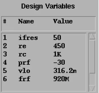
1. Set up the ne600p mixer cell fromdfII/samples/artist/rfExamples library.The design variable frf should be set to 920MHz.
2. Ensure that the sourcetype on the rf port is ’sine’ and the Amplitude (dBm) is set to prf. 3. Set up a PSS analysis. The beat frequency should be set to 40MHz. Set the number of
harmonics to 2 (only two harmonics are required to determine the 1 dB compression point). Sweep the prf parameter from -30 to 10 in 10 linear steps.
4. Set the Model Library path to include thedfII/samples/artist/models/ spectre/rfModels.scs file.
5. After running the simulation, call up the Waveform Calculator and the Results Browser.
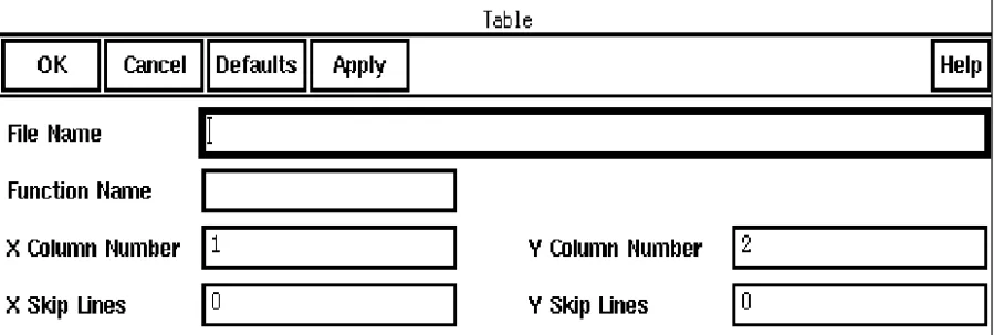
Click on schematic->psf->Run1->sweeppss_pss_fd-sweep->sweepVariable->prf->10->sweeppss-004_pss-fd.pss->Pif with the left mouse button. The following will appear in the calculator buffer:
v( "/Pif" ?result "sweeppss_pss_fd-sweep" ?resultsDir "~/simulation/ne600p/ spectre/schematic" ).
6. Click on Special Functions -> compression. The Compression form will be
displayed.
7. Enter Harmonic number=2. This is the second harmonic of the 40 MHz fundamental
frequency, which is the IF frequency (80MHz).
8. Enter Ext. Point (X) =-25 field to specify the extrapolation point of the waveform. The extrapolation point is the X axis value.
9. Enter Compression dB = 1 to specify the compression coefficient (N).
10. Click on the OK button.
11. Click the Evaluate Buffer button in the Calculator. The result appears in the Calculator
To use this function, you must type the line below in the CIW envSetVal("calculator" "oldexpr" ’boolean nil)
or set the calculatoroldexpr variable to nil in your.cdsenv file.
CompressionVRI Function
This function performs an Nth compression point measurement on a power waveform.
Use this function to simplify the declaration of a compression measurement. This function extracts the specified harmonic from the input waveform(s), and uses
dBm(spectralPower((i or v/r),v))to calculate a power waveform. The function then passes this power curve and the remaining arguments to the compression function to complete the measurement.
The compression function uses the power waveform to extrapolate a line of constant slope (dB/dB) according to a specified input or output power level. This line represents constant small-signal power gain (ideal gain). The function then finds the point where the power waveform drops N dB from the constant slope line and returns either the x coordinate (input referred) or y coordinate (output referred) value.
To use this function:
1. Define the voltage waveform in the buffer.
2. Choose compressionVRI in the Special Functions menu.
4. Type a value in the Extrapolation Point field to specify the extrapolation point for the
waveform. The default value is the minimum x value of the input voltage waveform. The extrapolation point is the coordinate value in dBm that indicates the point on the output power waveform where the constant-slope power line begins. This point should be in the linear region of operation.
5. Type a numerical value in the Load Resistance field. The default value is 50.
6. In the Compression dB field, type the delta (in dB) between the power waveform and
the ideal gain line that marks the compression point. The default value is 1.
7. Choose whether the measurement is for Input Referred Compression or Output
Referred Compression.
8. Click OK.
Convolution (convolve) Function
The convolve function computes the convolution of two waveforms.
1. Define the first waveform in the buffer.
2. Define the second waveform as the first stack element. 3. Choose convolve from the Special Functions menu.
The Convolution form appears.
Convolution is defined as
f 1 s( )f 2 t( –s)ds from
to
∫
f1 and f2 are the functions defined by the first and second waveforms.
Note: The convolve function is numerically intensive and might take longer than the other
functions to compute.
Threshold Crossing (cross) Function
The cross function computes the x-axis value xcross at which the nth crossing of the specified edge type of the threshold value occurs.
1. Choose cross.
The Threshold Crossing form appears.
2. Enter the threshold value of the waveform at which to perform the calculation.
3. In Edge Number, enter the number of the crossing at which to perform the calculation.
The integer you enter specifies which crossing is returned. (For example, 1 specifies the first crossing, and 2 specifies the second crossing.)
If you specify a positive integer, the count starts at the smallest x value of the waveform, and the search is in the direction of increasing x values. If you specify a negative integer, the count starts at the largest x value of the waveform, and the search is in the direction of decreasing x values. If you enter 0, all the crossings found are returned in a list.
4. Select an Edge Type to determine the crossing as the rising edge, falling edge, or either
edge.
5. Specify Number of Occurrences as multiple or single. The default setting is single,
which retrieves only one occurrence of a crossing event for a given waveform. If you select multiple, you can retrieve all occurrences of crossing for a given waveform, which you can later plot or print. The field Edge Number is dsabled if Number of
Occurrences is specified as multiple.
6. Specify Plot/print vs. as time or cycle. The default setting is time, which helps you
retrieve crossing data against time (or another X-axis parameter for non-transient data). For example:
time (s) cross(VT("/out") 2.5 0 0 t "time") (s) ---
---27.87n 27.87n 823.3n 823.3n 2.027u 2.027u 2.806u 2.806u
Here, time values refer to each timepoint on the waveform where the crossing event occurs.
The cycle option helps you retrieve crossing data against cycle numbers. For example:
cycle cross(VT("/out") 2.5 0 0 t "cycle") (s) ---
---1 27.87n 2 823.3n 3 2.027u 4 2.806u
Here, cycle numbers refer to the n’th occurence of the crossing event in the input waveform.
Frequency Voltage
Value xcross returned by cross function
Note: The value for this field is ignored when Number of Occurrences is specified as
single.
7. Click OK.
dBm Function
The dBm function performs the operation dB10(x) + 30
1. Enter the value in the buffer. 2. Select dBm.
Delay Function
The delay function computes the delay between two points or multiple sets of points in a waveform by using thecross function.
1. Enter the second waveform into the first stack register. 2. Enter the first waveform into the buffer.
4. For both waveforms, specify Threshold Value, Edge Number, Edge Type and
Periodicity for the specified edge.
5. For Number of Occurrences, select single or multiple to indicate whether you want
to calculate delay for one or more occurrences. If you select multiple, the delay is computed for the specified edges of the waveforms and also for the edges occuring at the periodic intervals (specified as Periodicity) for each waveform.
6. Specify Plot/print vs. as trigger time, target time, or cycle. The default setting is
trigger time, which helps you retrieve delay data against trigger time. Trigger time is the time when the first waveform crosses the specified threshold value.
For example:
cycle delay(VT("/out") 1.5 1 "rising" VT("/out") 1.5 2 "rising" 1 1 t "trigger") (s) --- ---18.19n 1.999u 2.018u 2.001u 4.018u 1.999u 6.018u 2.001u
Here, time values refer to each timepoint on the waveform where the threshold delay occurs.
Target time is the time when the second waveform crosses the specified threshold value. For example:
cycle delay(VT("/out") 1.5 1 "rising" VT("/out") 1.5 2 "rising" 1 1 t "target") (s) --- ---2.018u 1.999u Frequency Voltage Threshold value for WF1 Threshold value for WF2 WF1 WF2
delay = xcross2 - xcross1 xcross1 xcross2