THE APPLICATION OF TECHNICAL DEBT MITIGATION TECHNIQUES TO A MULTIDISCIPLINARY SOFTWARE PROJECT. Rachael Lee Luhr

THE APPLICATION OF TECHNICAL DEBT MITIGATION TECHNIQUES TO A MULTIDISCIPLINARY SOFTWARE PROJECT

by

Rachael Lee Luhr

A thesis submitted in partial fulfillment of the requirements for the degree

of

Master of Science in

Computer Science

MONTANA STATE UNIVERSITY Bozeman, Montana

©COPYRIGHT by

Rachael Lee Luhr 2015

DEDICATION

This thesis is dedicated to my parents, Mary and Donald Luhr. It was through their guidance and unwavering support that I choose to study Computer Science and to continue into graduate school. From practicing long division in the pick-up truck before elementary school to programming a robot for my sixth grade science fair project, they were always encouraging me to pursue my interests and follow my dreams. I hope I can continue to inspire others in the same way.

ACKNOWLEDGEMENTS

When I entered college, I had no intention of going to graduate school. When my advisor, Dr. Clemente Izurieta, gave me the opportunity to work on undergraduate research it changed my mind. It was with his guidance and support that I decided to continue my education and pursue a master‘s degree. I am so grateful for his patience to answer my questions and his high expectations which made me continually push myself to become a better student and researcher.

I would also like to thank the members of the Software Engineering Laboratory. Through our intelligent discourse, I have learned more than I thought possible. I am glad I got to go through this adventure with them, and wish them all luck while finishing their academic journeys. They have been amazing lab mates and friends.

A special thank you goes to Kevin Scott at Evans & Sutherland for his copious amounts of help with the Digistar 4 program and his patience with my learning. Without him, the visualization of this work would not have been possible.

Lastly, none of this would have been possible without the support of my parents, sister, and all my family and friends. They have always encouraged me to achieve my goals and had unwavering faith that I would do so. I would also like to thank my best friend and partner, whom I greatly admire and respect, Derek Reimanis. His love, kindness, and understanding have kept me going through times when I doubted myself, and I will be forever thankful.

TABLE OF CONTENTS 1. INTRODUCTION ...1 Motivation ...1 Summary of Approach ...1 Summary of Contributions ...3 Organization ...3 2. RELATED WORK ...5

Uncertainty in Technical Debt ...5

What is Technical Debt? ...5

How Do We Measure TD? ...6 Uncertainty in Calculations...9 Comparing Measures ...9 Propagation of Error ...10 Multivariate Uncertainty ...10 Modularity Violations ...10

What are Modularity Violations?...11

Importance of Replication in SE ...12

Effects of MV in Software ...12

3. BACKGROUND ...16

Network Exchange Objects ...16

What is NEO? ...16

How Does NEO Work? ...18

Hydrology ...19

Watershed Modeling ...19

4. APPROACH ...23

Particle Tracker Program Design and Development ...23

Technical Requirements...23

System Design ...26

The Particle Tracker Algorithm ...28

Validation ...30

Using SonarQube to Measure TD ...32

5. VISUALIZATION ...35

TABLE OF CONTENTS – CONTINUED Platform...35 Outreach ...36 Approach ...37 Multiple Currencies ...39 6. CURRENT RESEARCH ...41 Multiagent Systems ...41 Background ...41 In Hydrology ...44

An Integrated NEO Design ...45

Functional Requirements ...45

System Design ...46

7. CONCLUSIONS AND FUTURE WORK ...48

REFERENCES CITED ...49

APPENDICES ...55

APPENDIX A: On the Uncertainty of Technical Debt Measurements ...56

APPENDIX B: Natural Science Visualization using Digital Theater Software ...64

APPENDIX C: A Replication Case Study to Measure the Architectural Quality of a Commercial System ...71

APPENDIX D: Input and Output Tables from the Simplified Testing Graph for the Particle Tracker Algorithm ...84

LIST OF TABLES

Table Page

1. SQALE method of measuring technical debt ...8

2. Summary of different treatments between case studies ...13

3. Tau-b values for metric pairs ...14

4. The first five rows of the matrix database table ...24

5. Five rows of the model results database table ...26

LIST OF FIGURES

Figure Page

1. Technical Debt Quadrant ...6

2. How cells are connected in a NEO model ...17

3. Watershed delineation on a topographic map ...20

4. Inter-connected components of a river ...21

5. All four layers of links as plotted by R ...25

6. UML Component Diagram for the Particle Tracker program ...27

7. Specification file for the Particle Tracker program ...28

8. Java code for the randomization portion of the algorithm ...29

9. Simplified graph to test particle tracking conditions ...31

10. Sonar-properties.properties file...33

11. Duplications and Complexity score calculated by SonarQube ...33

12. Different technical debt scores calculated by SonarQube ...34

13. Screenshot of the Digistar 4 dashboard ...36

14. Screenshot of the Nyack Floodplain visualization...39

15. Visualization of heat and water currencies fluxing through a cube ...40

16. An example of how agents can be organized and interact ...43

LIST OF EQUATIONS

Equation Page

1. CAST Equation for Estimating Technical Debt ...8 2. Technical Debt equation including error ...9

NOMENCLATURE

DB – Database

DBMS – Database Management System

CAHN – Complex Adaptive Hierarchical Network

CERG – Computational Ecology Research Group

IDE – Integrated Development Environment

LOC – Lines of Code

LRES – Land Resources and Environmental Sciences

MAS – Multiagent System

MV – Modularity Violation

NEO – Network Exchange Objects

PT – Particle Tracking

SE – Software Engineering

SEL – Software Engineering Laboratory

SQL – Structured Query Language

TD – Technical Debt

ABSTRACT

The research described by this thesis uses contributions made to the technical debt community to create a high quality multidisciplinary software project under collaboration between computer scientists and hydrologists. Specifically, additions to the body of knowledge regarding technical debt and modularity violations are described. Technical debt is a metaphor borrowed from the financial domain used to describe the sacrifices that developers make in order to get software released on time. We looked at the uncertainty associated with technical debt measurements and expanded on well-known equations by investigating how errors propagate. We also looked at how modularity violations affect the overall architectural quality of a large-scale industrial software system. Modularity violations occur when modular pieces of code that are not meant to change together, do change together.

The second portion of the thesis applies the research learned from modularity violations and from the uncertainty investigations in technical debt measurements to a specific problem in hydrology to create a more accurate, modularized, and extensible particle tracking algorithm. We used SonarQube‘s technical debt software to further investigate technical debt measurements. We then visualized the modeling output from the particle tracking algorithm using high-tech digital theater software that was extended to accurately represent natural science visualizations. Finally, we describe the design necessary to seed the application of multiagent system theories and technologies to improve 3D hydrologic modeling.

INTRODUCTION

Motivation

Software projects are often the work of collaborations –field and industry domain experts approach computer scientists to solve problems. The need for the work summed up in this thesis was made apparent by hydrologists from the Department of Land Resources and Environmental Sciences at Montana State University. Hydrologists often collect large amounts of data from field work; which requires significant amounts of pre-processing and organization in order to accurately represent said knowledge. A well architected system forms a foundational framework that can be used to build extensibility through new approaches and explicability of results through behaviorally deterministic algorithms. This foundation is a critical requirement when interpreting large amounts of data. Simulation and modeling practices are widely used by hydrologists as an approach to quickly validate results and contrast hypotheses that require the evaluation of large amounts of data. By architecting high quality extensible architectures that use systematic approaches to carry out experiments we have an opportunity to help. The work herein uses computer science (and specifically, software engineering) theories and technologies to fill the needs of those hydrologists.

Summary of Approach

To address the hydrologists‘ problem of understanding their data, this work follows a two-prong approach. The first step is to enhance and improve the idea of

particle tracking by designing and implementing an efficient and accurate particle tracker algorithm that is closely linked with the currently used modeling framework. Particle tracking refers to the modeling of artifacts that can be aggregated to form a currency. A currency is a collection of artifacts that flow through a system according to some step function (typically time). The particles that flow through the system can be abstracted to be any token of interest; however, in this case study, it is limited to water particles. The latter are simple agents that traverse a graph (representative of their setting of use) and are commanded externally. A particle that is externally commanded can be thought of as a simple agent, and a particle that can make its own decisions can be thought of as smart. Whilst the current work focuses on simple agents, the algorithm is also on track to use multiagent systems theory to create more intelligent particles. Intelligent particles are able to make informed decisions and process information instead of relying on external programs.

The second step in the approach is to visualize the data received from the particle tracking algorithm. Visualization is a very powerful and useful tool in many areas, not just hydrology. However, when hydrologists can see how water is moving through a watershed, it provides insight to what hydrologic and/or non-hydrologic processes are taking place in that watershed. This is an invaluable tool when understanding such complex data.

While developing an implementation of the algorithm, it was essential to work under the guiding principles that drive high quality in software engineering. Two relevant areas that affect the quality of architectures, and that form a significant contribution to

this work, were studied. Technical debt and modularity violations are considered to be important characteristics of high quality systems. Both characteristics formed a precursor to beginning this project and were fundamental to its success. Research was conducted to advance the science by identifying ways to minimize the impacts of technical debt [1] and modularity violations [2] in the context of developing the particle tracking algorithm enhancements and its complementary visualization techniques [3].

Summary of Contributions

 Increasing knowledge in the uncertainty involved in technical debt measurement.

 Observing how modularity violations affect the architectural quality of large-scale industrial software.

 Developing a more accurate, modularized, and extensible particle tracking algorithm.

 Visualizing modeling output using high-tech visualization software that has been extended to accurately represent natural science visualizations.

 Designing and laying the framework to start applying multiagent system theories and technologies to improve 3D hydrologic modeling.

Organization

The rest of this thesis is organized as follows: Chapter 2 discusses related work involving technical debt and modularity violations in software projects. Chapter 3 provides background information on the Network Exchange Objects modeling

framework and why it is useful in the field of hydrology. Chapter 4 describes the

approach used when developing the particle tracker program and how it operates with the modeling framework. The work done with the visualization of models is presented in Chapter 5. Chapter 6 outlines the current and future research to be done in this area. Finally, Chapter 7 provides the conclusions of this work.

RELATED WORK

Uncertainty in Technical Debt

The understanding of the principles behind technical debt was critical in shaping this research. In order for developers to create valuable software while adhering to the best software engineering principles, technical debt must be understood and be at the forefront of design. If technical debt is accrued, they must also understand how much technical debt exists and how to eliminate it. In prior work [1], we discuss the uncertainty involved when measuring technical debt. The following two sections provide an abridged description of technical debt and why it is so difficult to measure.

What is Technical Debt?

Coined in 1992 by Ward Cunningham [4], the term ―technical debt‖ is a metaphor to describe the sacrifices that developers make in order to get software released on time. This metaphor is borrowed from the financial industry where sometimes, one needs to take on debt in order to advance. Like financial debt, when software needs to be refactored or redesigned, it costs extra time and money to make these fixes. However, sometimes incurring technical debt (like financial debt) is necessary. Martin Fowler [5] has shown that there are four main types of technical debt that can occur. The quadrant shown in Figure 1 illustrates these types of debt.

Figure 1. Technical Debt Quadrant [5].

It is especially difficult to measure and subsequently remove inadvertent technical debt. This occurs when the developers are making poor design decisions and are not even aware they are doing so. In cases when developers know they are acquiring technical debt, they are doing it deliberately. As the quadrant shows, this can be done recklessly or prudently. The ―best‖ kind of technical debt occurs deliberately and prudently. It must be stated that technical debt is not always incorrect and is sometimes even necessary.

Developers must ensure that if they are taking on technical debt, it needs to be done in a way that can be managed and understood. That way, like Seaman et al. mention in [6], technical debt data can then be used in important decision making strategies such as when (or if) a company needs to refactor its code.

How Do We Measure TD?

As stated in the previous section, technical debt is very difficult to measure. Curtis et al. [7] state that ―there is no exact measure of Technical Debt, since its calculation must be based only on the structural flaws that the organization intends to

fix.‖ However, many organizations may not be aware of the technical debt in their software or may not want to fix the technical debt they are aware of.

In [8], Ferenc et al. describe three types of software quality assessment models. These models are useful because they can provide developers with quantitative

information to assess the quality of their software. The three types of models are: Software Process Quality Models, Software Product Quality Models, and Hybrid

Software Quality Models. The difference between the first two types of models is that the first attempts to measure the process of software and the second attempts to measure the

product (that is, the software system itself). These types of models measure the quality of the product by combining different source code metrics.

Following this, there have been several different proposed ways to measure technical debt. Griffith et al. [9] performed a study to examine the relationship between several different methods of measuring technical debt and an external software product quality model. Several of these technical debt estimation methods will be discussed in the following paragraphs.

In 2012, Letouzey and Ilkiewicz introduced the Software Quality Assessment based on Life-cycle Expectations (SQALE) method [10]. SQALE is based on four main concepts: the quality model, the analysis model, the four characteristics (maintainability, changeability, reliability, and testability), and the indicators. Table 1 describes the

characteristics and how to solve the problems related to these characteristics. The authors give a remediation function that describes approximately how long it would take to fix

these problems. However, developers are free to change these functions based on their particular skills.

Table 1. SQALE method of measuring technical debt [10].

Characteristic Requirement Remediation microcycle Remediation function

Maintainability There is no commented-out block of instruction

Remove (no impact on compiled code)

2 minutes per occurrence Code indentation shall follow a

consistent rule

Fix with help of the integrated development environment (IDE) feature

2 minutes per file, regardless of the number of violations Changeability There is no cyclic dependency

between packages

Refactor with IDE and write tests

1 hour per file dependency to cut Reliability Exception handling shall not

catch null pointer exception

Rewrite code and associated test

40 minutes per occurrence Code shall override both

equals and hash code

Write code and associated test

1 hour per occurrence There is no comparison

between floating points

Rewrite code and associated test

40 minutes per occurrence No iteration variable are

modified in the body of a loop

Rewrite code and associated test

40 minutes per occurrence All files have unit testing with

at least 70% code coverage

Write additional test 20 minutes per uncovered line to achieve 70% Testability There is no method with a

cyclomatic complexity over 12

Refactor with IDE and write tests

1 hour per occurrence if measure is < 24; 2 hours if > 24 There are no cloned parts of

100 tokens or more

Refactor with IDE and write tests

20 minutes per occurrence

In 2011, the CAST Research Labs (CRL) published a report that highlighted the fact that companies are not budgeting for the millions of dollars‘ worth of technical debt that exists in their software products [11]. This report used the following equation to estimate the principal of technical debt in dollars, where principal is defined as the cost of fixing problems remaining in the code after it has been released.

Estimated Technical Debt Principal =

((((∑ high severity violations) x % to be fixed) x avg hours to fix) x $ per hour)) + ((((∑ med severity violations) x % to be fixed) x avg hours to fix) x $ per hour)) + ((((∑ low severity violations) x % to be fixed) x avg hours to fix) x $ per hour)) +

The authors of this equation purposefully leave the parameters adjustable so that each customer or company can customize the equation to fit their specific needs. The problem with this approach is that it leaves room for error if companies are unsure what values to use for the parameters.

Uncertainty in Calculations

Due to human factors, uncertainty does exist in measurements of technical debt. As the methods in the previous sections stated, there is no hard rule or set standard for how to calculate technical debt. In [1], we use techniques from physical sciences (like those discussed by Taylor [12]) and apply them to software engineering technical debt measurements. We use Equation 2 to calculate the measure of technical debt principal by using the developers best estimate of technical debt principal and adding (or subtracting) a margin of error or uncertainty.

Equation 2. Technical Debt equation including error [1]

Comparing Measures. Unlike the physical sciences, where we can use multiple physical tools and compare them to calibrate a measurement, tools that measure technical debt cannot be compared because measurement of technical debt is still in its infancy and we have not yet agreed on a common metric –all approaches use different equations. Using calculations that are unadjusted for error are uninteresting. By providing a measure of uncertainty along with the technical debt measurement, allows scientists to begin moving towards an understanding of the significance that certain factors have on the

response variable (i.e. technical debt); which would allow us to more accurately compare two (or more) measurements.

Propagation of Error. This error is very important to measure because it can propagate through technical debt measurements. In [13], Nugroho et al. propose calculations to measure aspects of technical debt. In [1], Izurieta et al. used these

equations to show this propagation of error. They discuss the propagation of uncertainty in sums, differences, products, and quotients of measured quantities.

Multivariate Uncertainty. Taylor [12] uses quadrature in formulas that need to deal with multivariate equations. This method is appropriate to use when the

measurements come from Normal or Gaussian distributions and are independent. While this is a good place to begin investigating, this type of calculation needs more validation within the field of software engineering.

Until we have agreed upon standards or tools to accurately measure technical debt, it is important to report the corresponding error in technical debt measurements. Additional work in this area is critical to further the understanding of technical debt and how it affects software projects.

Modularity Violations

Technical debt can appear in code in many different ways. In [14], Izurieta et al. evaluate four different types of debt and approaches to examine and mitigate this debt. This work is also extended in [15] to include more recent studies and findings. The four

indicators of technical debt discussed include design patterns and grime buildup [16] [17], code smells [18], ASA (automatic static analysis) issues [19] [20], and modularity violations [21]. All four of these areas deserve further attention so that we can gain more insight into technical debt. Their findings suggest that there exist significant gaps in technology, and that each technique is designed to measure different aspects of technical debt. At an architectural level, modularity violations are more relevant to the work

necessary to extend this thesis. In this section we focus on modularity violations and their importance in the technical debt landscape.

What are Modularity Violations?

Baldwin and Clark [22] define a module as ―a unit whose structural elements are powerfully connected among themselves and relatively weakly connected to elements in other units.‖ Modularity violations occur when two modules that are not expected to change together do change together. These violations are very important to recognize because understanding their consequences can lead to better design decisions and/or highlight the need for refactoring, thus reducing technical debt. However, early detection of modularity violations can be very difficult because their influence in the code is not always immediately apparent.

In [21], a tool called CLIO was designed and tested to detect modularity

violations. We conducted a replication case study [2] using this tool to test its efficacy at correctly detecting modularity violations and to increase the knowledge base surrounding modularity violations and their effect on technical debt.

Importance of Replication in SE

Experimental replication studies are important in a field such as empirical software engineering [23] [24] because they help build consensus around emerging theories. Observing and studying software projects often, if not always, also involve the study of humans. Human behavior can be extremely unpredictable and difficult to replicate. This makes conducting a controlled experiment very challenging. By performing replication case studies, we can increase the confidence of ideas.

The replication of case studies, such as the one performed by Reimanis et al. [2], are not as common as replications of experiments. However, they are just as important. Case studies take place in the real world (in-vivo), and observations are made in the context of their domains. This tends to be typical of software engineering studies because controlled experimentation is cost prohibitive. The observation of historical data (a longitudinal approach) is also common in empirical software engineering studies, and occurs when we observe phenomena over various versions of software. This type of information is invaluable when attempting to understand how projects actually evolve. In our replication study we borrowed terminology from existing information on

experimental replication studies [25].

Effects of Modularity Violations in Software

We conducted a replication of a study by Schwanke et al. in [26]. Both projects were industrial software products. Our code base was a commercial software system developed by a local bioinformatics company – Golden Helix [27]. They gave us access to their code base because they were interested in learning about potential modularity

violations in their designs. They specifically wanted us to point out potential deficiencies in their code organizational structure.

We had five major treatment differences from the original study. Table 2 summarizes these differences. The first major difference is the programming language that the projects were written in. The baseline project was written in Java and our project was written in C++.

Table 2. Summary of different treatments between case studies [2]

Factor Baseline Project Our Project

Programming Language

Java C++

# of Developers Up to 20 Up to 11 Project Lifetime 2 years 4 years

# of Source Files 900 3903

KSLOC 300 1300

The difference of treatments in this factor brought about interesting complications in the study because Java projects are structured differently than C++ projects. Because of this, we had to slightly modify our definition of a module. In this study, we defined a module as a directory. This choice was based on Parnas et al.‘s definition [28]. The terms module and directory are used interchangeably. We also had to group C/C++ source files and header source files together. This is because developers expect source files and their related header files to change together. Our study was only concerned with unexpected changes across modules.

The other differences between the baseline project and our project include the number of developers, project lifetime, number of source files, and kilo-source lines of

code (KSLOC). Our project had fewer developers, but a longer lifetime and is larger in terms of source files and LOC.

In order to gather data on this project, we followed the work of Schwanke et al. [26] and looked at seven different metrics; which were gathered for all file pairs across all seven versions of Golden Helix‘s software. These metrics included: file size, fan-in, fan-out, change frequency, ticket frequency, bug change frequency, and pair change frequency. The definitions of these metrics can be found in [2]. We used CLIO to gather measurements for these metrics by looking at the source code and the version history of the project. Following the baseline study, Kendall‘s tau-b rank correlation measure was used [29]. Table 3 shows the tau-b value calculated for each metric pair in releases 7 and 7.5 of the software.

Table 3. Tau-b values for metric pairs [2]

R7+R7.5 Fan-in Fan-out File size Changes Tickets Bugs

Fan-in 1 0.257 0.301 0.331 0.328 0.464 Fan-out 0.257 1 0.441 0.417 0.416 0.637 File size 0.301 0.441 1 0.293 0.273 0.510 Changes 0.331 0.417 0.293 1 0.972 0.858 Tickets 0.328 0.416 0.273 0.972 1 0.857 Bugs 0.463 0.637 0.510 0.858 0.857 1

Highlighted cells with a value of 0.6 or greater indicate strong correlation [30]. Most of the highlighted results were expected. Changes, bugs, and tickets have

significant correlation values. An unexpected result was the correlation between bugs and fan-out. This number shows that as the fan-out of a file pair increases, the number of bugs associated with that pair also increases. These results are consistent with the baseline case

study [26], adding to the knowledge of how modularity violations occur and how well CLIO detects them.

Developers at Golden Helix were unsurprised by the findings of our study. Many of the files that were causing modularity violations were known to be heavily dependent on other files, and some modularity violations were intentional. However, it was

reassuring for the baseline developers to receive this information because it meant that there were few modularity violations occurring that they were not expecting. The latter exemplify prudent and deliberate technical debt.

BACKGROUND

Network Exchange Objects

Network Exchange Objects (NEO) is a software framework designed to facilitate development of complex natural system models [31] where models are represented as graphs that can carry and communicate data represented as flows of currencies. NEO began a re-engineering phase of development at Montana State University in 2009 as a joint venture between the Computer Science Department and the Department of Land Resources and Environmental Sciences (LRES). NEO can be used as a general-purpose modeling tool applicable to many domains [32].

What is NEO?

NEO was designed to study systems that can be described as ―complex adaptive hierarchical networks‖ (CAHNs). CAHNs are complex systems through which

information is stored and routed and can be represented in a graphical form. CAHNs are constructed of cells that are linked by edges and are structured hierarchically. Cells represent system components. These cells can be defined as any physical component of a system. This can range from discrete sections of a riverbed (e.g., a model of a watershed) to an abstract representation of cars (e.g., a vehicular communication network). Any conceptual structural component the modeler is interested in can be represented as a cell.

The edges in a CAHN represent the interaction between cells. This is where the information about the behavior of exchanges between cells is stored. For example, in a watershed model, the interaction between cells might include the flow of water, exchange

of heat, or flow of sediment. In a vehicular communication model, the modeler might be interested in the signals being exchanged between cars. The behavior (described as calculations) for how these exchanges occur, is located in the edges of the graph.

There are two faces associated with each edge. Edges can contain behavior that is synchronous; that is, the behavior of a face on one side of the edge is reflected on its counterpart on the opposite face (e.g., the signals between two communicating cars), or asynchronous, where each face has its own unique behavior (e.g., the flow of sediment in a riverbed). This is illustrated in Figure 2. Having ―to‖ and ―from‖ sides of edges helps distinguish the flow of information.

Figure 2. How cells are connected in a NEO model [33].

Within this graphical representation of a system model, currencies flow from the ―from‖ side of an edge to the ―to‖ side. A currency represents anything within the model that is being exchanged between components of the modeled system (e.g., radio signals, water, sediment, energy, economic capital, nutrients, or any other resource that is of interest to the system). These currencies are then manipulated as they flow (or flux) between cells and edges in the defined matrix network, representing the effect entities have on the flow. For example, if Figure 2 was describing a watershed model where the

cells are discrete patches of the river and the behavior located in the edges describes the flow of water (i.e., the currency) between patches, then the water would be flowing downriver from Cell 1 to Cell 2.

There are several vocabulary words that are used in conjunction with NEO [33]. The following is an abridged selection of key definitions.

 Holon – Cells, edges, and/or faces that correspond to real-world components of the modeled system.

 StateVal – A variable within a holon that can be altered.

 Dynam – (Auto/Manual/Init) A static or dynamic method (i.e., an algorithm) in which a stateVal is manipulated. This is where the currency behavior is defined.

 Currency Package – A package written in the Java programming language that defines the behavior of a currency through a set of dynams.

 Model – A combination of the NEO framework and the necessary currency packages which are to represent the desired system.

How Does NEO Work?

The core algorithm of NEO uses a Trade-Store-Update cycle approach. This process determines the order of operations for the dynam calculations. In the Trade phase, currencies that are fluxed between cells are calculated within each edge and their values are saved to the currency stateVals within that edge. In the Store phase, dynams that are located in cells update their currency stateVals based on the values that were calculated in the Trade phase. Finally, in the Update phase, all automatically refreshing values update their stateVals.

To develop and execute a NEO model, the following software requirements are necessary. First, a development environment of the Java programming must be installed on the machine. Second, an Integrated Development Environment (IDE) must be used. IDEs provide a platform that allows the organization of files that correspond to NEO concept implementations. Whilst not essential, it provides a significant aid when managing models. Third, a database must exist in order to store information about the model inputs and outputs.

Hydrology

One natural science field that lends itself well to the NEO modeling framework is hydrology - specifically, the study of movement, distribution, and quality of water. Water flowing in a river exemplifies NEO functionality: the river is the structure that makes up the network and the water is the currency that fluxes through the system.

Watershed Modeling

The need for a system like NEO was made apparent by hydrologists from the LRES Department at Montana State University. Simulation modeling allows scientists to test many hypotheses in a relatively cheap environment, providing significant insights into specific factors that can then be further explored and validated through real world field studies, which are more expensive. Therefore, there are great advantages in hydrological modeling. Much of the research in this area is done to improve scientist‘s ability to predict or forecast the effects of land-use and climate change on the water balance, streamflow variability, and water quality. Hydrologists are particularly interested

in the flow of water through a watershed. According to Dingman [34], a watershed is defined as the ―area that appears on the basis of topography to contribute all the water that passes through a given cross section of a stream.‖ An example of watershed delineation is shown in Figure 3.

Figure 3. Watershed delineation on a topographic map [34].

The floodplain of interest (i.e., experimental unit) of this study is the Nyack Floodplain located in Western Montana near Flathead Lake. The Nyack Floodplain includes the watershed of the middle fork of the Flathead River. This area has been the focus of considerable research in the state of Montana and the surrounding areas. This research spans many topics including migratory patterns of bull trout [35], how the river affects grizzly bear diets [36], and the structure of the river itself [37]. In 2012, Helton et al. studied the temperature and dissolved oxygen dynamics of this system [38]. After the

implementation of NEO, this work was extended and provided the basis for the data used in this thesis.

Helton et al. [39] were especially interested in the residence time of water within the Nyack floodplain. Rivers are composed of surface and subsurface flow. Water that becomes part of the subsurface (also known as ground-water) generally has longer residence time. The topography of the landscape creates an immense influence on the movement of water [40]. This leads to the idea of breaking up the watershed into smaller blocks where water acts similarly within those blocks. Figure 4 shows how the river breaks down into these separate components.

Figure 4. Inter-connected components of a river [41]. Figure Copyright © 2004 John Wiley & Sons, Ltd. Reproduced by permission.

In order to model this watershed in NEO, the river was broken down into discrete patches. The ―cells‖ represent patches and are depicted in Figure 4 as nodes drawn in the center of a corresponding polygon. The ―edges‖ are drawn as straight lines connecting the cells. There are three layers in this watershed, as is indicated in Figure 4 (the surface layer, the hyporheic layer, and the aquifer layer). This allows for representation of

horizontal water flow, horizontal and vertical subsurface flows, and the vertical exchanges between subsurface and surface waters.

APPROACH

Particle Tracker Program Design and Development

To visualize how water flows through a floodplain, hydrologists use a method known as particle tracking. Particles can be thought of as independent agents that flow through the floodplain and behave according to domain specific equations. Agents can be configured to report on information according to predefined criteria. In the case of

particles they are configured to output their position at various time steps. This output can then be used to gain insight on how water may actually be moving. The design of the tracking algorithm uses current and modern object oriented techniques that encompass high quality characteristics (i.e., low technical debt, use of design patterns, and use of object oriented design principles). The implementation is written in the Java

programming language.

Technical Requirements

There are three technologies necessary to run the particle tracking software: the Java 81 developer‘s kit and runtime environment, an Integrated Development

Environment (IDE), and a database. The development of our project used Eclipse 4.2.1 Juno2 and PostgreSQL 9.23 as the Database Management System (DBMS) with full support for the Structured Query Language (SQL).

1 _{https://java.com/en/download/} 2 _{http://www.eclipse.org/downloads/} 3 _{http://www.postgresql.org/download/}

Output from a NEO model run is stored in a database. The particle tracking program uses the information stored in the database tables to make informed decisions on how to move the particles. The database contains two tables. One includes the

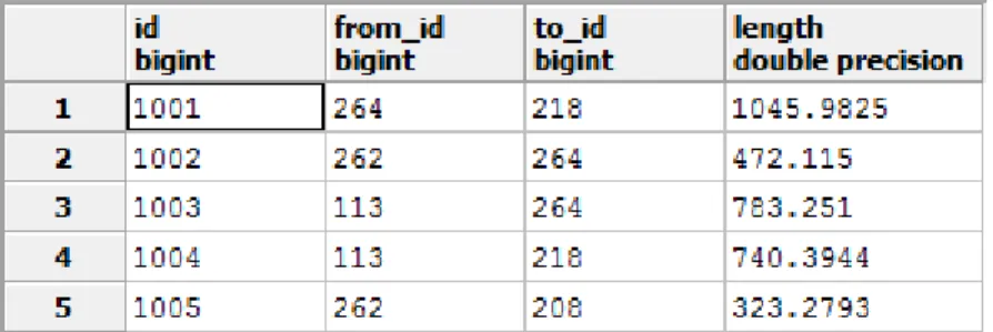
information to form the matrix (or the structure) of the river system. A portion of this table is shown in Table 4. It consists of four columns that must be named: id, from_id, to_id, and length. ‗id‘ is a unique integer that corresponds to the id of the link connecting two nodes. ‗from_id‘ is an integer that corresponds to the id of the originating node that a link is coming from. ‗to_id‘ is an integer that corresponds to the id of the destination node that a link is going to. ‗length‘ is a value of type double that corresponds to how long the link is (in meters). Links are directional because direction can be critical in most flux networks. For example, we do not want water flowing ―up‖ river.

Table 4. The first five rows of the matrix database table.

The information in this matrix table forms four layers of the floodplain. These layers are surface water, shallow groundwater, deep groundwater, and soil. This data was pulled into the R statistical software4 and plots were created for each layer. These images can be easily compared to the visualization to ensure that the data was consistent across all programs (NEO, the particle tracker, and the visualization software). Figure 5 shows

the R plots for the soil links, deep groundwater links, shallow groundwater links, and surface water links.

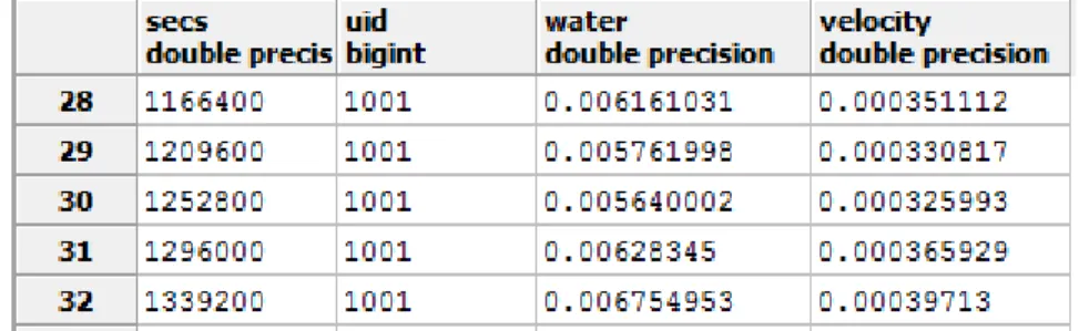
The second database table, partially shown in Table 5, provides the results from the NEO model run. This table also consists of four columns: secs, uid, water, velocity. ‗secs‘ is the time (in seconds) associated with that particular line of output. This

instantiation of the model run output every 43,200 seconds, or 12 hours. ‗uid‘ is the link id. This value corresponds to the link id from the matrix information table. The

combination of ‗secs‘ and ‗uid‘ is what makes a row in the table unique. ‗Water‘ is the flux value of water flowing through that link at that particular time. ‗velocity‘ refers to how quickly that water is moving down the link. The equations that were used to represent the physical principles behind the water flow are described by Walton et al. [42] and Poole et al. [41].

Table 5. Five rows of the model results database table.

System Design

As mentioned in the previous section, the NEO output tables must be located in a database and, along with a specification file, provide the input for the particle tracker program. The program also outputs to a database table located in the same DBMS as the NEO output tables. Figure 6 shows the UML component diagram for the particle tracker program.

Figure 6. UML Component Diagram for the Particle Tracker program

The specification input file is where the user specifies how many ―particles‖ they would like released, where they would like them released, and how often they want the particles to report on their current location. Figure 7 displays this specification file (in this case called RiverInfo.txt). The first line, DataTimeInterval, is time interval that coincides with the NEO output data. The ReleaseInfomation contains the cell in the matrix (referred to in this context as a node) where the user wants the particles released, how many particles the user wants released, and the release time for those particles, respectively. The third line in the file specifies when to start reporting particle tracker information. The user may not always want to start reporting at the beginning of the model, so this allows for flexibility. The ReportInterval on line 4 describes how often to report output from the particle tracker. The accuracy of a simulation improves as this report interval decreases. Finally, the last line, Destination, describes cells (or nodes) in the matrix where the user wants to see the particles will exit the simulation (in this case, as the furthest downriver point of the floodplain.

Figure 7. Specification file for the Particle Tracker program

Once the environment and the specification file are correctly specified, users may run the particle tracker program by selecting the Main.java class in Eclipse (or IDE of choice) and pressing the run button.

The Particle Tracker Algorithm

The movement of particles is based on available links, velocity, and flux. Particles start by moving along the links connected to the specified nodes. To move, particles query the database for the velocity along that link at that particular time. The particle then calculates how far it should move down the link based on how much time has passed multiplied by the velocity.

A particle knows it has reached the end of a link when its movement has exceeded the link‘s length. At arrival to a node, the particle queries the database to see which links are available for selection by observing which links contain the current node as the ―from node‖. Once there is a list of known available links, the particle must choose which one to select to continue its trajectory.

To more accurately represent a real system, a level of randomness is inserted into the choices that particles make when they reach a specific node. The program queries the database to find the flux values for all the available links at the current time. It then uses a

weighted formula to cumulatively sort these links from smallest flux value to largest (on a scale from 0.0 to 1.0). This is compared to a random number generated by the program (also between 0.0 and 1.0). The particle chooses the first link that has a higher weighted flux value than the random number. See Figure 8 for the portion of the code that handles this logic.

Figure 8. Java code for the randomization portion of the algorithm

At the time step stated on line 4 of the specification file, the particle reports its particle id number, the id of the link it‘s currently traversing, the current time, and its position on the link. This information is written to a database table in order to provide easy access to the output once the particle tracker is finished. Table 6 shows the first six rows of this output table. You can see that the particle reports every 500 seconds (as specified). When the particle reaches the end of link 1741, it chooses link 1743 as its new link to follow its trajectory.

Table 6. Six rows of the particle tracker program output table

Validation

The Nyack watershed model‘s matrix table contains a total of 3054 lines and its model results table contains a total of 369,534 lines. To validate that the particle tracker algorithm was working correctly, we created a smaller scale model that contained all the possible conditions present in the larger model. In collaboration with hydrology domain experts, the following represent the conditions that required testing:

1. Particles had to choose links correctly based on weighted flux with some element of randomness.

2. If the velocity reaches 0 in the middle of the link, the particle would stop moving, but would keep reporting its position.

3. If a particle comes to a junction where none of the available outgoing links have a flux value greater than 0, the particle will wait at the junction until the flux becomes greater than 0.

4. If a particle comes to a junction and there is a link with positive velocity but the link is the wrong direction, the particle should never choose to go down this link.

The graph constructed to test these conditions is shown in Figure 9. The node ids and link ids are shown on the graph. A model results database table was constructed to serve as an oracle that would have similar output to a NEO model run. This table also had the above conditions built into it. The particle tracker was run with those two tables as input and the specification file tailored to fit this model. The particles were released at node 1, reported every 100 seconds, and expected to arrive at nodes 6, 7, 8, or 9. After the particle tracker finished executing, the output was validated by hand to ensure that the four conditions were met and particles were behaving as expected. See Appendix D for input tables and output from this example.

Using SonarQube to Measure TD

The particle tracker program was developed with the goal to minimize technical debt. As mentioned in Chapter 2, there are many approaches to measuring technical debt within a software system. To measure the technical debt in the particle tracker system, the SonarQube platform was used [43]. SonarQube evaluates technical debt by examining various potential disharmonies in a system, including: duplications, coding standards, lack of coverage, potential bugs, complexity, documentation, and design. It calculates several scores: a Technical Debt score (measured in man days – how many 8 hour developer days it would take to fix all the issues), the SQALE rating [10] (from A-E, A being the highest), and the Technical Debt Ratio (how much technical debt the project has versus how large it is).

In order to get results from SonarQube, the user must download and run the SonarQube Server (which allows users to view their results online) and the SonarQube Runner (which launches the program and allows for projects to be analyzed). The user must also provide a sonar-properties file. The properties file used is shown in Figure 10. Once the SonarQube Server is running and the SonarQube Runner has been launched and ran against the project with the sonar-properties file, the user can see the output by navigating to http://localhost:9000 in their browser.

Figure 10. Sonar-properties.properties file

The particle tracker program consists of 8 files (or classes), 45 functions, and a total of 802 lines of code (LOC). Figure 11 shows the amount of duplications and the complexity score as calculated by SonarQube.

Figure 11. Duplications and Complexity Score calculated by SonarQube [43]

Figure 12 displays the SQALE Rating, Technical Debt Ratio, and the amount of Technical Debt of the program. SonarQube also allows the user to click on the ―Issues‖ measure to navigate to a dashboard where users can observe what the issues are and

where they are located in the files. This allows for much quicker fixes and provides a visual tool for the user to see if they are making identical mistakes.

Figure 12. Different technical debt scores calculated by SonarQube [43]

On the SonarQube website, there is also a formula for calculating the cost of remediating observed technical debt. The default value is parameterized at $500 per developer day. Using this value, the cost to reduce technical debt in the particle tracker program would be $2125. However, this value is configurable in the SonarQube

platform. If we chose a different amount for this project, for example, the average pay of an intern in the Bozeman area ($160/day), the reported cost would be $680.

VISUALIZATION

Motivation

One of the main problems associated with the understanding of complex scientific data is mentally visualizing what processes are occurring. Given this difficulty, many scientists rely on models and visualizations to aid their understanding. The need for visualization is one of the main reasons why the work in this thesis began. One of the best (and most intuitive) ways to portray the hydrological model to a larger audience is with visualization.

Platform

The platform used as a vehicle for these visualizations is Digistar 4 [44], one of the most advanced and successful digital planetarium platforms. It was developed by Evans and Sutherland Company, based in Salt Lake City, UT. Digistar 4 was chosen because it was easily accessible and has a powerful graphics engine that provided the necessary requirements to accurately visualize the particle tracking model. It was also intuitive and user friendly. Figure 13 is a screenshot of the Digistar 4 dashboard.

Figure 13. Screenshot of the Digistar 4 dashboard

Outreach

Another large reason of why Digistar 4 was chosen for this project is the potential it had for outreach. The Taylor Planetarium is part of the Museum of the Rockies, which in turn is a department of Montana State University. The Museum of the Rockies is the most visited indoor attraction in Montana, with an annual attendance of 100,000 visitors. The Taylor Planetarium seats 60,000 of those visitors each year. The Taylor Planetarium is the only planetarium building in Montana, making it a premier travel destination. The museum acts as an outreach arm for the land grant university, and it is tasked to educate all ages, from adults to school children. The planetarium had been recently upgraded from Digistar 2 to Digistar 5 (the newest version of the software at the time of

publication). The upgrade allowed for visualizations developed on the Digistar 4 platform to be run in Taylor Planetarium. This spurred the idea of creating an MSU Minute show

to run in the planetarium before a normal planetarium show. The MSU Minute was an idea from the planetarium director to highlight research occurring at MSU5. The actual show lasted 2-4 minutes and was shown in front of various audiences for several months. Other departments at MSU had already taken advantage of this opportunity to display their research.

Starting in September 2013, an MSU Minute describing the initial work from this thesis was displayed in front of a planetarium show for approximately six months [45]. This allowed the work done by CERG (Computational Ecology Research Group) and SEL (Software Engineering Laboratory) to be viewed by thousands of visitors to the museum. Outreach in the sciences is important because it allows for a way to portray complex information in a relatable and understandable way to an audience unfamiliar with many of the complicated details.

Approach

To import the particle tracking model into Digistar 4, the information in the NEO database and the output from the particle tracker program had to first be converted into the correct Digistar file formats. These are proprietary formats and not easily readable. A Java program was created to serve as a filter that converts readable data to proprietary information needed for Digistar. The files required by Digistar 4 include: a graph file, which tells Digistar how to set up the model in 3D space; a frequency file, which contains how many particles are fluxing through the system and the duration (measured in time

steps) that each particle exists within the model; and a position file, which has all the particle location information in 3D space during each moment in time.

Once the model information was in the correct file formats, Digistar 4‘s scripting language was used to create a mock planetarium show. This allowed the model to be shown in dome view (or visualization view). The scripting language and Digistar‘s advanced interface provided the necessary functionality to tweak parameters in the model in order to calibrate it to the right position and the correct size. The user can also control the flow rate of the particles, their size, and their color. It is also possible to navigate through the model in real time and to zoom in and out on selected areas. It can be looked at from above, below, or inside. This feature provided many useful options when creating the MSU Minute.

Figure 14 is a snapshot of what the Nyack floodplain visualization looks like in Digistar 4. There is an image in the background of the Nyack overlaid with the structure of the river. The particles are directly following along the edges of the matrix imitating the way that the water would flow.

Figure 14. Screenshot of the Nyack Floodplain visualization

Multiple Currencies

While not necessary for the Nyack visualization, many models may require that more than one currency flux through the system at one time. For example, if the modeler also wanted to see the heat exchange within the river, then they would need to add a second currency (heat) to the model. The work for adding this functionality was shown in [3]. The ability to visualize models with multiple currencies is essential for many reasons.

It improves the interpretation of the visual data. It also allows the modeler to focus on one of the currencies or both at the same time. This is achieved by setting the opacity of the unwanted currency to zero. Furthermore, because the currencies are input into Digistar 4 as separate files, the user can adjust the color and flow rate to be different for each currency. Figure 15 shows an example of a heat currency (red) and a water currency (blue) flowing through a simple cube-shaped matrix. The currency particles are different sizes and are moving at different speeds.

CURRENT RESEARCH

Multiagent Systems

As is, the particle tracking program serves as a valuable commodity to

hydrologists, and while care has been taken to minimize the amount of technical debt inherent in the system, additional work is required. Specifically, and to increase the modularity of the system, the particle tracking algorithm needs to be fully integrated into the current NEO architecture. After a series of design discussions with hydrologists, we observed that particles behave as separate ―agents‖ that make independent decisions. This prompted the study of multiagent systems.

Background

Whilst research on multiagent systems (MAS) began in the early 1980‘s, it only really began to organize itself in the mid 1990‘s. Since then, with the advent of the Internet and advances in computer science, multiagent system work has grown into the large field that it is today. A MAS is characterized as a system where there is no global system control, data is decentralized, computation is asynchronous, and each agent has incomplete information or capabilities for solving the problem, and thus, has a limited viewpoint.

An ―agent‖ is a computer system that is capable of independent action on behalf of its user or owner [46]. In order for agents to be considered intelligent, they have to possess two important abilities: they need to be capable of autonomous actions and they need to be capable of interaction with other agents. These interactions include

cooperating, coordinating, and negotiating. To facilitate MAS technology, we require mechanisms that allow agents to synchronize and coordinate their activities at run-time. Weiss et al. [47] defined four different classes of agents:

1. Logic-based agents: in which the decision about what action to perform is made via logical deduction.

2. Reactive agents: in which decision-making is implemented in some form of direct mapping from situation to action.

3. Belief-Desire-Intention agents: in which decision making depends on the manipulation of data structures of the agent.

4. Layered architectures: in which decision-making is realized via various software layers, each of which is more or less explicitly reasoning about the environment at different levels of abstraction.

Research indicates that the type of agent architecture that would best fit this work is the layered architecture, which is currently the most popular class of agent

architectures available. Figure 16 illustrates how agents can be organized and how they interact with each other and their environment.

Figure 16. An example of how agents can be organized and interact [46]

One important aspect of a MAS is the ability for agents to communicate with each other. Because agents are autonomous, they can neither force other agents to perform actions, nor affect the properties, and thus the internal state of other agents. Agents are able to perform communicative actions in an attempt to influence other agents

appropriately. These agents must also agree upon an ontology and a protocol for sharing information. Negotiation and bargaining are two important types of communication. Negotiation is a form of interaction in which a group of agents with conflicting interests try to come to a mutually acceptable agreement over some outcome. Bargaining is often solved by argumentation among agents [48]. Argumentation can be seen as a reasoning process consisting of the following four steps: Constructing arguments from available information, determining the different conflicts among the arguments, evaluating the

acceptability of the different arguments, and concluding, or defining, the justified conclusions [49].

Below is a list of situations when agent based solutions are appropriate [50] and why they are highly relevant additions to this project:

1. When the environment is open, or at least highly dynamic, uncertain, or complex – NEO models are dynamic and complex. You often have a large mesh network (i.e., a graph) with many currencies fluxing that need to updated, tracked, and reported on.

2. When agents are a natural metaphor – A hydrological model lends itself to agent metaphors.

3. Distribution of data, control, and expertise – In NEO models, each cell and/or edge holds different information. This makes the data distributed. In Hydrology

The idea of using multiagent systems in the field of hydrology is not new [51]. The vernacular used in the field refers to them as agent-based models. These types of models work well in natural sciences because they represent complex systems that can be broken down into individual components and allow for communication between these components.

Today, there is no standard in how to create these agent-based models [52]. Many authors believe that creating this standard is an important step to wide-spread use of agent-based models in the natural sciences. Volker et al. released an article in 2006 [53] describing a standard protocol for describing agent-based models. The protocol was

widely used (having over 1000 citations) and in 2010, they published a review and update to the protocol [54]. Agent-based models have been widely used in the field of hydrology ( [55], [56]) and highly relevant to the continuing refinement of the particle tracker and other currency algorithms.

An Integrated NEO Design

Research in multiagent systems revealed that the particle tracker program was already very close to representing intelligent agents. As particles move through a matrix, they observe their surroundings and make informed decisions about routes based on information that they collect. Thus, our investigations suggest that the particle tracker would be more useful to modelers when fully integrated with the NEO framework.

Functional Requirements

After speaking to NEO modeling experts, they outlined several functional

requirements that the enhanced and fully integrated particle tracker program would need to adhere to. In this context, particles will now be referred to as ―agents‖. The functional requirements are:

1. Deploy agents: An agent manager will be able to either deploy agents at the beginning of a model or during model run time.

2. Track and move: Each agent will track its location in relation to nodes and/or links at run time as the agent moves through the network.

3. Sense and record conditions as an agent moves through a model: An agent will check its velocity and flux values in the current edge and will decide where to move based on that information.

4. Alter external values within the model: An agent will have the ability to update a counter in a node to track how many agents have passed through that node.

5. Retain information: A central agent manager will store the information that each agent collects.

6. Report: An agent will be able to either report during a simulation or a-posteriori.

7. Exit simulation: An agent manager within the model will handle the departure of agents.

8. Visualize simulation: The output collected by agents will be visualized in a visualization system.

System Design

Figure 17 depicts a UML class diagram of a possible design of the particle tracker. It employs intelligent agents, and uses NEO terminology to seamlessly integrate all components under the existing NEO architecture. The design encompasses all the functional requirements and was validated by NEO experts and hydrologists. After integration, agents become part of NEO, and will be configurable at run time to allow for more functionality and understandability of NEO models.

CONCLUSIONS AND FUTURE WORK

The work presented in this thesis contributes to the technical debt and modularity violation knowledge base –both topics of significant attention in the software engineering community. We used this knowledge and applied it to a multidisciplinary software

project. The project was verified by using SonarQube‘s technical debt measurement tool and by domain experts in both software engineering and hydrology.

An accurate and extensible particle tracking algorithm was developed. The particle tracking program was run using hydrological data from the Nyack floodplain in northwestern Montana. The data was generated by NEO, a simulation software

framework designed to facilitate development of complex natural system models.

Further, the output from the particle tracking program was visualized using digital theater software –Digistar 4. The visualization of the data provided a unique and valuable

alternative to understanding how the movement of the particles behaved and allowed modelers a gather greater understanding of their models.

The work presented in Chapter 6 introduced currently ongoing work to transform the particle tracking algorithm to exhibit additional properties inherent in multiagent systems that track intelligent agents. Although the design for integrating the particle tracking program with intelligent agents with NEO is completed, it has not been implemented. Another essential feature that would need to be added is the ability for agents to communicate with each other. In addition to functional enhancements, the particle tracking algorithm should be tested on models outside the field of hydrology to ensure that it is applicable to other domains.

[1] C. Izurieta, I. Griffith, D. Reimanis and R. Luhr, "On the Uncertainty of Technical Debt Measurements," in International Conference on Information Science and Applications, 2013.

[2] D. Reimanis, C. Izurieta, R. Luhr, L. Xiao, Y. Cai and G. Rudy, "A replication case study to measure the architectural quality of a commercial system," in 8th

International Symposium on Empirical Software Engineering and Measurement, 2014.

[3] R. Luhr, D. Reimanis, R. Cross, C. Izurieta, G. C. Poole and A. Helton, "Natural Science Visualization Using Digital Theater Software: Adapting Existing

Planetarium Software to Model Ecological Systems," in 2013 International Conference on Information Science and Applications, 2013.

[4] W. Cunningham, "The WyCash Portfolio Management System," ACM SIGPLAN OOPS Messenger, vol. 4, no. 2, pp. 29-30, 1992.

[5] M. Fowler, 14 October 2009. [Online]. Available:

http://www.martinfowler.com/bliki/TechnicalDebtQuadrant.html. [Accessed 10 February 2015].

[6] C. Seaman, Y. Guo, C. Izurieta, Y. Cai, N. Zazworka, F. Shull and A. Vetrò, "Using technical debt data in decision making: Potential decision approaches," in Third International Workshop on Managing Technical Debt, 2012.

[7] B. Curtis, J. Sappidi and A. Szynkarski, "Estimating the Principal of an Application's Technical Debt," IEEE software, vol. 6, pp. 34-42, 2012.

[8] R. Ferenc, P. Hegedus and T. Gyimothy, "Software Product Quality Models," in

Evolving Software Systems, Berlin, Springer-Verlag, 2013, pp. 65-100.

[9] I. Griffith, D. Reimanis, C. Izurieta, Z. Codabux, A. Deo and B. Williams, "The Correspondence between Software Quality Models and Technical Debt Estimation Approaches," in Sixth International Workshop on Managing Technical Debt, 2014. [10] J.-L. Letouzey and M. Ilkiewicz, "Managing technical debt with the SQALE

method," IEEE software, vol. 6, pp. 44-51, 2012.

[11] "CAST Report on Application Software Health," CAST, 2011.

[13] A. Nugroho, J. Visser and T. Kuipers, "An empirical model of technical debt and interest," in 2nd Workshop on Managing Technical Debt, 2011.

[14] C. Izurieta, A. Vetrò, N. Zazworka, Y. Cai, C. Seaman and F. Shull, "Organizing the technical debt landscape," in Third International Workshop on Managing Technical Debt, 2012.

[15] N. Zazworka, C. Izurieta, S. Wong, Y. Cai, C. Seaman and F. Shull, "Comparing four approaches for technical debt identification," Software Quality Journal, vol. 22, no. 3, pp. 403-426, 2014.

[16] C. Izurieta and J. M. Bieman, "How software designs decay: A pilot study of pattern evolution," in First International Symposium on Empirical Software Engineering and Measurement, 2007.

[17] C. Izurieta and J. M. Bieman, "A multiple case study of design pattern decay, grime, and rot in evolving software systems," Software Quality Journal, vol. 21, no. 2, pp. 289-323, 2013.

[18] M. Fowler, Refactoring, imporving the design of existing code, Pearson Education India, 2002.

[19] A. Vetro, M. Torchiano and M. Morisio, "Assessing the precision of findbugs by mining java projects developed at a university," in 7th IEEE Working Conference on Mining Software Repositories, 2010.

[20] A. Vetro, M. Morisio and M. Torchiano, "An empirical validation of FindBugs issues related to defects," in 15th Annual Conference on Evaluation & Assessment in Software Engineering, 2011.

[21] S. Wong, Y. Cai, M. Kim and M. Dalton, "Detecting software modularity violations," in 33rd International Conference on Software Engineering, 2011. [22] C. Y. Baldwin and K. B. Clark, Design rules: The power of modularity (Vol. 1),

MIT Press, 2000.

[23] F. J. Shull, J. C. Carver, S. Vegas and N. Juristo, "The role of replications in

empirical software engineering," Empirical Software Engineering, vol. 13, no. 2, pp. 211-218, 2008.

[24] A. Brooks, M. Roper, M. Wood, J. Daly and J. Miller, "Replication's role in software engineering," in Guide to advanced empirical software engineering, Springer