Phase Synchronization Analysis of Event-Related Brain Potentials in Language Processing

(1)

Institut f¨

ur Physik

Arbeitsgruppe Nichtlineare Dynamik

Phase Synchronization Analysis

of Event-Related Brain Potentials

in Language Processing

Dissertation

zur Erlangung des akademischen Grades

doctor rerum naturalium

(Dr. rer. nat.)

im Fach Physik / Nichtlineare Dynamik

eingereicht an der

Mathematisch-Naturwissenschaftlichen Fakult¨

at

der Universit¨

at Potsdam

von

Carsten Allefeld

Potsdam, M¨

arz 2004

(2)

(3)

Zusammenfassung

Das Forschungsthema Synchronisation bildet einen Schnittpunkt von Nichtlinearer Dyna-mik und Neurowissenschaft. So hat zum einen neurobiologische Forschung gezeigt, daß die Synchronisation neuronaler Aktivität einen wesentlichen Aspekt der Funktionsweise des Gehirns darstellt. Zum anderen haben Fortschritte in der physikalischen Theorie zur Entdeckung des Phänomens der Phasensynchronisation gef ührt. Eine dadurch motivierte Datenanalysemethode, die Phasensynchronisations-Analyse, ist bereits mit Erfolg auf em-pirische Daten angewandt worden.

Die vorliegende Dissertation kn ¨upft an diese konvergierenden Forschungslinien an. Ih-ren Gegenstand bilden methodische Beitr¨age zur Fortentwicklung der Phasensynchronisa-tions-Analyse, sowie deren Anwendung auf ereigniskorrelierte Potentiale, eine besonders in den Kognitionswissenschaften wichtige Form von EEG-Daten.

Die methodischen Beiträge dieser Arbeit bestehen zum ersten in einer Reihe spezia-lisierter statistischer Tests auf einen Unterschied der Synchronisationsstärke in zwei ver-schiedenen Zuständen eines Systems zweier Oszillatoren. Zweitens wird im Hinblick auf den viel-kanaligen Charakter von EEG-Daten ein Ansatz zur multivariaten Phasensynchro-nisations-Analyse vorgestellt.

Zur empirischen Untersuchung neuronaler Synchronisation wurde ein klassisches Ex-periment zur Sprachverarbeitung repliziert, in dem der Effekt einer semantischen Verlet-zung im Satzkontext mit demjenigen der Manipulation physischer Reizeigenschaften (Schrift-farbe) verglichen wird. Hier zeigt die Phasensynchronisations-Analyse eine Verringerung der globalen Synchronisationsstärke f ür die semantische Verletzung sowie eine Verstärkung f ür die physische Manipulation. Im zweiten Fall läßt sich der global beobachtete Synchro-nisationseffekt mittels der multivariaten Analyse auf die Interaktion zweier symmetrisch gelegener Gehirnareale zur ückf ühren.

Die vorgelegten Befunde zeigen, daß die physikalisch motivierte Methode der Phasen-synchronisations-Analyse einen wesentlichen Beitrag zur Untersuchung ereigniskorrelier-ter Potentiale in den Kognitionswissenschaften zu leisten vermag.

Abstract

The topic of synchronization forms a link between nonlinear dynamics and neuroscience. On the one hand, neurobiological research has shown that the synchronization of neuronal activity is an essential aspect of the working principle of the brain. On the other hand, recent advances in the physical theory have led to the discovery of the phenomenon of phase synchronization. A method of data analysis that is motivated by this finding—phase synchronization analysis—has already been successfully applied to empirical data.

The present doctoral thesis ties up to these converging lines of research. Its subject are methodical contributions to the further development of phase synchronization analysis, as well as its application to event-related potentials, a form of EEG data that is especially important in the cognitive sciences.

The methodical contributions of this work consist firstly in a number of specialized sta-tistical tests for a difference in the synchronization strength in two different states of a sys-tem of two oscillators. Secondly, in regard of the many-channel character of EEG data an approach to multivariate phase synchronization analysis is presented.

For the empirical investigation of neuronal synchronization a classic experiment on lan-guage processing was replicated, comparing the effect of a semantic violation in a sentence context with that of the manipulation of physical stimulus properties (font color). Here phase synchronization analysis detects a decrease of global synchronization for the seman-tic violation as well as an increase for the physical manipulation. In the latter case, by means of the multivariate analysis the global synchronization effect can be traced back to an inter-action of symmetrically located brain areas.

The findings presented show that the method of phase synchronization analysis mo-tivated by physics is able to provide a relevant contribution to the investigation of event-related potentials in the cognitive sciences.

(4)

(5)

Introduction

The topic of synchronization has recently achieved an outstanding role in neurobi-ology and cognitive science as well as in nonlinear dynamics. In cognitive neuro-science, synchronization is more and more considered to be one of the basic mecha-nisms of brain function, from visual perception up to highest cognitive processes. In physics, the long known phenomenon of synchronization of periodic oscillators has in the last years been extended to chaotic systems. These recent advances have led to a cooperation of the two research fields which forms the background of the present thesis.

This chapter gives a short introduction into this converging research. It for-mulates the main theoretical ideas that have led to the current interest in synchro-nization processes in neuroscience and summarizes a number of important studies that have been published in this context. This includes the findings of the physical theory of synchronization in nonlinear dynamics and the application of the result-ing analysis methods to neurophysiological data. Finally, the chapter states the specific aims of this work and gives an outline of the following.1

1.1 Temporal binding

Neurobiological research has shown (cf. Engel et al., 1991) that in the visual cortex there exists a hierarchy of neurons that detect increasingly complex features of the scene registered by the eyes. On the simplest level, they just copy the activation patterns of sensory neurons in the retina, but subsequent cells react to contrasts, movements, linear structures in a specific direction, and so on, each in a specific area of the visual field. If one assumes that this hierarchical pattern of accumulat-ing complexity is the functional principle of the whole brain, one has to conclude that at the highest level for each object that is possibly relevant to the organism there exists a single dedicated neuron that detects the special complex combination of properties this object consists of. Since such a scheme leads to an absurdly high number of combinations, it calls for far more neurons than are actually present in the brain (the “combinatorial explosion”), and it implies the strange notion that every contingent item of the world gets hard-coded into the brain (presumably during maturation), which has been caricatured by the idea of the “grandmother neuron”—a neuron that is active if and only if one’s grandmother is present.

On the other hand, for complex perception and cognition it is not sufficient that only basic stimulus features are detected in specialized brain areas. If a number of

1_{In this introduction, the understanding of the concepts referred to has to be presumed. Many of}

them will be explained in Ch. 2.

(8)

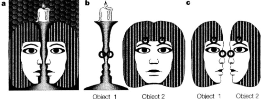
Figure 1.1:The concept of binding, illustrated by a “bistable” image. The image (a) has two possible interpretations: a face partially occluded by a candlestick (b), or two opposing faces (c). Both interpretations are distinguished by the way the edges that are detected at different places (marked by bold circles) are associated with each other to make up a contour—that is, how they are “bound” into object representations. Reproduced with permission from Engel et al. (2001), Dynamic predictions: Oscillations and synchrony in top-down processing. Nature Reviews Neuroscience, 2(10), Box 2. Copyright c2001 Macmillan Magazines Ltd. and c 1990 Palgrave Macmillan.

objects is perceived at the same time, and an activation pattern indicates the pres-ence of a certain set of stimulus features in the perception, there is no information about what features combine with which other features to make up the different objects (the “superposition catastrophe”). For instance, if there is a green ball and a red cube, the detection of “ball”, “cube”, “green”, and “red” could also be inter-preted as the presence of a red cube and a green ball. This necessity to specifically combine detected features into object representations is called thebinding problem (see Fig. 1.1). Because of the combinatorial constraint, binding cannot be achieved by the activity of neurons that are specifically sensitive to certain feature combi-nations. There has to be a means to encode the belonging-together of low level feature representations directly into the corresponding neuronal activity. That is, the alternative to the representation of an object by a detector neuron is its repre-sentation by an assembly of associated neurons that may be distributed over large areas of the brain.

Based on theoretical considerations (cf. von der Malsburg, 1985) as well as ani-mal experiments and an increasing number of findings in human neurophysiologi-cal data (see below), it is nowadays widely believed that the mechanism of binding employed in the brain is synchronization, ortemporal binding. While the activity of single neurons consists of bursts of firing (considered stronger the higher the fir-ing rate is), in most cases these bursts have oscillatory character. Accordfir-ing to the theory of temporal binding the activation of an assembly consists in the syn-chronization of the oscillatory activity of the associated cells. Since this temporal adjustment of firing activity of the cells is not necessarily affecting their individual mean firing rates, synchronization is suitable as a marker of belonging-together of features that are represented by the single neurons.

Though the concept of binding has been introduced in the context of percep-tion to understand the mechanism of sensory integrapercep-tion (of features into an object representation) and segmentation (of one object from another), today the theory of binding has to be seen in the broader context of thefunctional integrationof special-ized, spatially separated brain areas (cf. Varela et al., 2001). Large-scale cooperation in the brain seems to be necessary to achieve perception-related object representa-tions as well as more complex cognitive processes like the planning of acrepresenta-tions, the understanding of music and language, or for being conscious.

(9)

1.1 Temporal binding 9

References: Von der Malsburg (1985) introduces the idea of dynamic neuronal con-nectivity patterns as the basis of brain function. Von der Malsburg and Schneider (1986) describe neural synchronization as a means of sensory segmentation under the title of a “Correlation Theory” of brain function. (Interestingly, von der Malsburg (1995) argues that temporal binding is not only present in real brains, but is also efficient in improving the capabilities of artificial neural networks.) Damasio (1990) gives a model of memory re-trieval by synchronous activation of distributed neural networks, representing the different modality-related aspects of a recollection in the respective specialized brain areas. Varela (1995) discusses the concept of temporal binding (synchrony) in relation to cognitive opera-tions, wherein distributed cell assemblies underlie the coherence of cognition. Singer (2000) proposes that the brain uses two complementary strategies for representations: single cells specific to frequently occurring items of low complexity and transient cell assemblies for infrequent high-complexity items, while the relatedness of distributed neurons in the latter case is encoded by the synchronization of their responses. Engel et al. (2001) discuss experi-ments on synchrony in the context of a “dynamicist” idea of top-down processing of stimuli. They give an explanation of the functional role of synchrony (temporal coding) in the oper-ation of the brain, concerning the causes as well as consequences of synchrony. Varela et al. (2001) propose phase synchronization over multiple different frequency bands as a mech-anism of large-scale integration in the brain, to enable the emergence of coherent behavior and cognition. Thompson and Varela (2001) discuss the concept of synchronous cell assem-blies in the context of their “enactive” approach to the theory of consciousness. Engel and Singer (2001) as well as Singer (2001) investigate the relevance of temporal binding for the understanding of consciousness in the sense of sensory awareness.

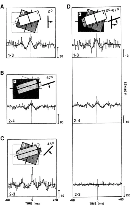
Following early theoretical approaches pointing to this direction, it was a num-ber of pioneering studies around 1990 that provided concrete evidence for the ex-istence of a temporal binding mechanism in the brain. These studies were mainly based on single cell and multi-unit recordings in the visual cortex of cats. Engel et al. (1991) give a review of experiments performed by their group (see there for further references). They found oscillations on the spike burst level in the fre-quency range 40–60 Hz with synchronizations that were specific to neurons with similar feature preferences. Especially compelling was their demonstration (see Fig. 1.2) of a simple form of sensory integration (by synchronization) and segrega-tion (by desynchronizasegrega-tion), i.e. direct evidence for the theory of temporal bind-ing. Similar results were obtained by another group; see Eckhorn et al. (1991) for a review and references.

These findings in animal experiments have inspired studies aimed at demon-strating synchronized activity in response to sensory and cognitive processing in humans. Because measurements on the cellular level are strongly invasive and can only in special cases be applied to human subjects, most of the studies have used EEG (electroencephalography, see Sec. 2.1) and similar data. Since EEG sig-nals represent the summed up activity of large local neuron populations, the band power (signal power in a selected frequency band) of the EEG response at a single recording site may be regarded as an indirect measure of synchronization within this population. Terminology related to this interpretation dates back to the in-vestigation of event-related changes in alpha band power starting in the 1970s, so-called event-related desynchronization and synchronization (cf. Pfurtscheller, 1998). In contrast to this, most newer studies have been oriented at the findings in the cat visual cortex and therefore have focused on band power in the gamma range (above 30 Hz).

References: Lutzenberger et al. (1994) find reduced band power for the perception of pseudowords (word-like sounds without a meaning) compared to words in the EEG gamma band; Pulverm ¨uller et al. (1996) repeat this finding for the MEG (magnetoencephalogram) gamma and beta band. Herrmann et al. (1999) report increased EEG gamma band power

(10)

Figure 1.2:Temporal binding in the cat visual cortex. Activity was measured from four cells that are detecting moving bars, with preferences regarding the orienta-tion of the bars of 157◦ _{(1), 67}◦ _{(2), 22}◦ _{(3), and 90}◦_{(4). Cross-correlograms of}

signals from pairs of cells are shown; an oscillatory cross-correlogram indicates synchronization. A)–C) Moving bars at different orientations cause synchroniza-tion between those cells that are activated. D) Two superimposed moving bars at orientations 0◦_{and 67}◦_{cause synchronization in cell pairs 1-3 and 2-4, but not}

be-tween cells 2 and 3. That is, neuron activities are synchronized only if they respond to the same object. Reproduced with permission from Engel et al. (1991), Tempo-ral coding by coherent oscillations as a potential solution to the binding problem: Physiological evidence, Fig. 5. In Schuster, editor,Nonlinear Dynamics and Neuronal Networks. Copyright c1991 Wiley-VCH.

(11)

1.2 Synchronization 11

for Kanizsa figures compared to similar visual stimuli without illusory contours. Herrmann and Mecklinger (2000) find increased MEG gamma band power for (visually presented) target stimuli compared to other stimuli. Lachaux et al. (2000) investigate LFP (local field potentials) gamma band responses to stimulation in a visual discrimination task. For further references see M ¨uller (2000), who gives an overview of the findings regarding gamma band responses.

Even if changes in local synchronization are indicated by changes in EEG band power, it still is an indirect measure and results are confounded with changes in the overall activity of the underlying neuron population. Though local synchro-nization effects like those found in the cat visual cortex cannot be expressly de-tected in EEG because of its low spatial resolution, EEG data seem to be feasible to investigate long-range synchronization between different brain areas as an indi-cator of their functional integration. Going a step beyond band power analysis, a number of studies have appliedcoherence(the correlation coefficient applied in the frequency domain) as a linear measure of bivariate synchronization. Coherence gives frequency-specific information on the degree of linear dependency between pairs of signals recorded at different sites. Other than most studies on band power, many of these studies report findings that are not confined to the gamma band.

References: Sarnthein et al. (1998) find increased EEG coherence in the theta band in a delayed response task and relate it to working memory operation. Miltner et al. (1999) report increased EEG gamma band coherence in an associative learning task, between those brain areas that are processing the two classes of stimuli given. Weiss et al. (1999) find dif-ferent coherence patterns in the EEG alpha-1 and beta-1 band for the processing of concrete vs. abstract nouns and sentence processing vs. pseudo speech. Von Stein and Sarnthein (2000) review several different studies on EEG band power and coherence and argue for a relation between the spatial scale on which synchrony-mediated functional integration takes place and the frequency band of the involved oscillations; these range from the theta to the gamma band. Schack et al. (2000) interpret the phase component of coherence in the EEG alpha-1 band; in the experiment, abstract nouns are visually and auditorily presented to the subject for memorization. Weiss and M ¨uller (2003) give a review of language pro-cessing research that is employing coherence: clinical studies on dyslexia, studies on word processing, text processing, and sentence processing.

1.2 Synchronization

By most authors, the mechanism of temporal binding as introduced above is de-scribed as synchronization of neuronal oscillations, that is as the dynamical adjust-ment of the rhythms of different oscillators (see Sec. 2.3). The theory of synchro-nization processes has a long tradition in physics, having been founded in the 17th century by Huygens for the case of periodic oscillators. In recent years the theory has been updated in the context of nonlinear dynamics and especially regarding the synchronization of chaotic oscillators. (For an introduction and further refer-ences, see Pikovsky et al., 2001). Here, Pecora and Carroll (1990) have shown that sufficiently strong coupling may cause two chaotic oscillators to follow identical trajectories (so-called complete synchronization). Subsequent research has led to the discovery by Rosenblum et al. (1996) of a specific form of chaotic synchroniza-tion that has become especially important for the investigasynchroniza-tion of neuronal pro-cesses: the phenomenon ofphase synchronization. In this case, a small coupling of the oscillators causes an adjustment of their phases, while the amplitudes remain uncorrelated and chaotic.

References: The first investigations of phase synchronization and related phenomena have been performed in numerical simulations, mainly employing R ¨ossler oscillators:

(12)

Ro-senblum et al. (1997) describe lag synchronization as an intermediate regime between phase and complete synchronization. Pikovsky et al. (1997) give a broad discussion of phase syn-chronization of chaotic oscillators. Pikovsky et al. (1996) investigate phase synsyn-chronization in a population of globally coupled chaotic oscillators and Osipov et al. (1997) in a lattice of chaotic oscillators. Zhou and Kurths (2002) find phase synchronization induced by com-mon noise. Zaks et al. (1999) describe imperfect phase synchronization between noniden-tical chaotic oscillators.—Phase synchronization has also been demonstrated in laboratory experiments and in models of as well as empirical data from natural systems, including the human body: Parlitz et al. (1996) observe phase synchronization of chaotic R ¨ossler oscilla-tors implemented in an electronic circuit. Rosa et al. (2000) show chaotic phase synchroniza-tion in a plasma discharge tube, DeShazer et al. (2001) in a laser array. Wang et al. (2000) describe phase synchronization and clustering in globally coupled chaotic electrochemical oscillators. Blasius et al. (1999) find phase synchronization in models of spatially extended ecological systems, Lunkeit (2001) in climate models. Paluˇs et al. (2000) investigate synchro-nization between the sunspot cycle and the solar inertial motion. Bhattacharya et al. (2001) apply phase synchronization and other nonlinear analysis methods to intensity oscillations of chromospheric bright points. Sch¨afer et al. (1999) show phase synchronization between the heart beat and the respiration cycle. Tass et al. (1998) demonstrate phase synchronization in MEG and muscle activity in Parkinsonian patients. Laird et al. (2002) describe synchro-nization between fMRI (functional magnetic resonance imaging) data and the presentation of a stimulus.—For a comprehensive overview of the literature on chaotic synchronization, see Boccaletti et al. (2002).

As noted above, in a number of studies synchronization in EEG has been inves-tigated using the coherence measure. This use can be justified by the observation that in the synchronization of two periodic oscillators, their phases are adjusted to each other while the amplitudes are constant. In this case, synchronization can be detected using coherence because the phase adjustment leads to an increased cor-relation of the two time series. But, as Tass et al. (1998) point out, synchronization of two oscillators is not equivalent to the linear correlation of two signals that is measured by coherence. If the participating oscillators are chaotic and in the phase synchronized regime, such that their amplitudes are varying with time but are not correlated to each other, the noise inherent in the amplitudes will reduce coher-ence changes related to synchronization. On the other hand, if the amplitudes of the two oscillators are changing with time in a regular way (for instance, because the number of neurons recruited for the local oscillator increases or decreases) and similar changes take place in both sites, such an amplitude correlation will cause an increase of coherence that is not related to synchronization.2

For these and related reasons, coherence is not to be regarded as a specific mea-sure of synchronization. Because the core of synchronization is the adjustment of phases and not of amplitudes, it should be detected by a measure neglecting ampli-tude variations (see Sec. 3.3). Such methods of data processing, that are necessary to specifically detect phase synchronization and that are applicable to synchroniza-tion in general, are calledphase synchronization analysis.

References: In the last years, there has been an increasing number of studies in cog-nitive neuroscience employing measures of phase synchronization for the analysis of EEG and similar data: Rodriguez et al. (1999) show specific patterns of long-range phase syn-chronization in the EEG gamma band related to the perception of upright vs. upside-down “Mooney” faces (black & white outline pictures of faces). Lachaux et al. (1999) find large-scale and local LFP phase synchronization in a visual discrimination task. Haig et al. (2000) demonstrate a late response in the degree of global and regional EEG gamma band phase 2_{Empirical evidence supporting these considerations is given by Quian Quiroga et al. (2002), who}

report that phase synchronization analysis (among other nonlinear methods) differentiates better be-tween different degrees of synchronization in rat EEG than linear measures.

(13)

1.3 Aims and outline 13

synchronization for task-relevant vs. irrelevant stimuli. Bhattacharya and Petsche (2001) find increased EEG gamma band phase synchrony in musicians while listening to mu-sic. Braeutigam et al. (2001) describe events of stimulus-locked MEG gamma band activ-ity associated with a semantic violation. Breakspear (2002) presents evidence of nonlinear contributions to the EEG based on phase synchronization analysis. Chavez et al. (2003) apply network cluster analysis to MEG phase synchronization relations in a binocular ri-valry experiment.—Another field in which phase synchronization analysis is effective and increasingly popular is the clinical evaluation of EEG, especially related to epilepsy: Mor-mann et al. (2000) find changes in phase synchronization before the onset of an epileptic seizure. Jerger et al. (2001) review the effectivity of several different nonlinear measures for seizure prediction and find that phase synchronization provides the most robust indicator. Le Van Quyen et al. (2001b) give an overview of nonlinear methods in seizure prediction including the approach based on phase synchronization. By Lee et al. (2003), EEG phase synchronization analysis is also proposed as a means of investigating the neural basis of schizophrenia.

1.3 Aims and outline

The subject of the present thesis can be specified related to the research summa-rized above in a number of different respects:

1) As a contribution to nonlinear dynamics, this work is analyzing empirical data obtained from a natural system (the human brain), but not investigating details of the theory of synchronization or specific phenomena in numerical simulations of model systems.

2) The data are obtained by EEG, and therefore describe the electrical activity of the brain on a relatively large-scale, or coarse-grained level. This is in con-trast to studies analyzing signals recorded at single cells or in small neuron populations, by macroelectrodes inside of the skull (LFP), or by MEG.

3) This work is interested in synchronization effects correlated with cognitive processes. In this it differs from studies on pathological conditions like epi-lepsy, where neuronal synchronization comes into view as a mainly physio-logical phenomenon.

4) Accordingly, the data are collected following the experimental paradigm of cognitive science, that is comparing the effects of slightly different versions of a cognitive process. Practically this means that responses are related to different classes of stimuli, each of which is realized many times. This form of EEG recording is called event-related potential (ERP).

5) The subject matter of the main experiment is defined by research interests of psycholinguistics. This choice has been determined by the author’s coopera-tion in the interdisciplinary DFG research group “Conflicting Rules”, part B1: “Diagnosis in Language Processing”. In this respect, this work tries to make theory and methods of physics useful for the purposes of another scientific discipline.

6) Regarding methodology, this work is looking for explicit effects of phase syn-chronization in the EEG. This is in contrast to the use of the band power and the coherence measure, that for reasons given above are only of limited use for the detection of synchronization processes.

(14)

The aims of this thesis are twofold: to adapt and apply the methods of phase syn-chronization analysis to event-related EEG data, and at the same time to contribute to these methods in a way that is also relevant in other fields of application.

The composition of the text is as follows:

In Ch. 2, the concepts underlying this work are introduced. This includes the basics of electroencephalography (Sec. 2.1), the definition of event-related poten-tials as well as an explanation of the established form of ERP analysis (Sec. 2.2), and the main topics of synchronization theory (Sec. 2.3). Since the research re-ported in the following lies at the intersection of (at least) two different disciplines, the purpose of this introductory chapter is to lay a common ground for readers with different backgrounds.

Chapter 3 presents elements of the data analysis method used here that are still of a basic nature, but that could have been done in another way: an algorithm em-ployed to reduce correlations in EEG due to mixing (Sec. 3.1), the use of wavelets to determine the instantaneous phase of a time series (Sec. 3.2), and the statistical measure of synchronization strength (Sec. 3.3). These elements represent decisions that continue the specification of the author’s approach sketched above.

In the next two chapters, contributions to the methods of synchronization ana-lysis are presented. Chapter 4 discusses a number of different approaches to test for statistically significant changes in synchronization strength between two oscil-lators. Methods of increasing precision, but also increasing complexity are intro-duced, explained and checked in numerical simulations.

In Ch. 5, an approach to multivariate phase synchronization analysis is derived and discussed, including a check of the underlying model in a numerical simula-tion. As a first empirical test of the method, an experiment on the visual process-ing of illusory contours (Sec. 5.2) was performed. Here, the multivariate analysis proves to deliver useful results in showing the emergence of a synchronization cluster as a response to the visual presentation.

The subject of the last chapter (Ch. 6) are empirical findings obtained by syn-chronization analysis of event-related potentials in language processing. A clas-sic experiment comparing the effect of a semantic incongruity in a sentence con-text with that of a physical mismatch (Kutas and Hillyard, 1980b) was replicated. The stimulus presentation is shown to elicit a transient increase of synchronization strength. Each type of deviation causes a specific modification of the basic pattern of synchronization.

(15)

Chapter 2

Basic Concepts

In this chapter, the concepts that are defining the subject matter of this work are introduced and explained. The data to be analyzed are obtained by electroen-cephalography; some technical and physiological aspects of this are described in Sec. 2.1. In the form of event-related potentials (Sec. 2.2), EEG is conceptualized as a random process (with respect to experimental events). The standard method of ERP analysis and its main findings are explained, especially in relation to cog-nitive processes. This method is to be supplemented by a new analysis procedure that looks for phase synchronization between brain areas. An introduction to the physical theory of synchronization focused on phase synchronization is given in Sec. 2.3.

2.1 Electroencephalography

The electroencephalogram (EEG) is the derivation and recording of time-varying voltages on the human scalp that are generated by the electrical activity of the brain, especially the neocortex (following Nunez, 1995). The (neo-) cortex or “gray matter” is the phylogenetically newest part of the brain; its functions include sen-sory and cognitive information processing, motor control, and conscious experi-ence. The cortex consists of a thin (2–3 mm) layer of neuronal tissue that is partly stretched out under the skull, partly folded into itself thereby increasing its surface. (Fig. 2.1)

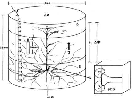
80 % of the neurons in the neocortex are so-called pyramidal cells, whose cell bodies are roughly of pyramidal (or rather conical) form. Pyramidal cells and the other neurons in the cortex are locally connected by short-range intracortical fibers (ca. 1 mm long) as well as globally connected by long-range corticocortical fibers (up to 20 cm), the latter making up the “white matter” directly below the cortex. Only a comparatively small amount of fibers comes out of or leads into other parts of the brain. The pyramidal cells are oriented perpendicular to the cortex surface and organized in local groups called columns, as well as larger populations, the so-called macrocolumns of ca. 3 mm diameter and containing 105_{to 10}6_neurons.

(Fig. 2.2)

The electric field of the cortex is caused by the current flows within a pyramidal cell and between it and the neighboring extracellular medium, making the cell an electrical dipole along its axis. Because of their parallel orientation, simultaneous activation of many pyramidal cells generates large correlated dipole layers whose electric field can be measured on the scalp (Fig. 2.1). Since this field reflects the de-gree of simultaneous activation in the local neuron population, the EEG recorded at a scalp electrode can be regarded as a relatively direct measure of the neocortical

(16)

Figure 2.1:Recording of EEG and MEG (magnetoencephalography). The EEG electrode is attached to the scalp surface and separated from the cortex by scalp tissue and skull. The EEG is most sensitive to correlated dipole layers in that parts of the cortex that lie directly under the skull (the so-called gyri; a–b, d–e, g–h). Reproduced with permission from Nunez (1995), Quantitative states of neocortex, Fig. 1-4. In Nunez, editor,Neocortical Dynamics and Human EEG Rhythms. Copy-right c1995 Oxford University Press.

Figure 2.2:A macrocolumn containing up to 106 _{neurons, with one pyramidal} cell shown explicitly. The insert shows a synaptic input that is causing microcur-rent sources and sinks. In EEG, the effect of the macroscopic net curmicrocur-rent density ~

J of macrocolumns is measured in the form of a potential difference∆Φ. From Nunez (1995), Fig. 1-11. Reproduced with permission from Sato, editor, Magne-toencephalography, Raven Press. Copyright c1990 Lippincott Williams & Wilkins.

(17)

2.1 Electroencephalography 17

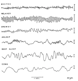
Figure 2.3:Characteristic EEG rhythms, depending on the state of consciousness. From Nunez (1995), Fig. 1-6. Reproduced with permission from Penfield and Jasper, Epilepsy and the functional Anatomy of the Human Brain, Little, Brown. Copy-right c1985 Lippincott Williams & Wilkins.

function of the underlying cortex area.

The spatial resolution of EEG lies roughly between 1 and 5 cm. This is markedly lower than the resolution that can be obtained with electrodes directly on the cor-tex surface (the so-called electrocorticogram applied in brain surgery patients), be-cause scalp electrodes have a distance of about 1 cm from the cortex and bebe-cause of the low conductivity of the skull that causes a smearing of the potential distribu-tion (Nunez, 1981, Ch. 1 & 8). This loss in resoludistribu-tion between cortex and scalp can in part be compensated for by different methods of postprocessing of EEG data (for a description of the “spherical spline Laplacian” algorithm used in this work, see Sec. 3.1). With high density electrode arrays and efficient postprocessing, the possible resolution of scalp EEG lies in the order of magnitude of macrocolumns, making them the natural theoretical units of cortical dynamics from the point of view of EEG interpretation (Nunez, 1995). For the purposes of this work, this ob-servation also specifies the spatial scale of the neuronal oscillators whose operation is to be examined in synchronization analysis.

The temporal resolution of EEG lies at about 1 ms, its spectral content being in the range from below 1 Hz up to approximately 100 Hz. The spectral composi-tion of EEG depends strongly on the state of consciousness, with a low-amplitude broadband spectrum being typical for awake persons with open eyes or perform-ing cognitive tasks (Fig. 2.3 & Fig. 2.4, “excited”). The EEG spectrum is traditio-nally differentiated in a number of frequency bands: delta, below 4 Hz; theta, from 4 to 8 Hz; alpha, from 8 to 13 Hz; beta, from 13 to 30 Hz; gamma, beyond 30 Hz (Fig. 2.4). Some of these wave bands are associated with characteristic dominant rhythms, the most prominent being the alpha rhythm, a high-amplitude sinusoidal oscillation of about 10 Hz that is coherent over posterior areas and that is observed in awake but relaxed subjects with closed eyes (Fig. 2.3 & Fig. 2.4, “relaxed”). EEG amplitudes are in the range from 10 to 100µV (Niedermeyer, 1998).

EEG electrodes are positioned according to the International 10-20 System that originally defined 21 locations but that has been updated by the American

(18)

Elec-0 20 40 60 10−5 10−3 10−1 101 spectral density / Hz −1 f / Hz relaxed 0 20 40 60 10−5 10−3 10−1 101 spectral density / Hz −1 f / Hz excited

Figure 2.4:EEG power spectral density (electrode CZ). Gray lines indicate the bor-ders between the frequency bands delta, theta, alpha, beta, and gamma. “relaxed”: The subject is resting with closed eyes. Note the strong peak at about 9 Hz corre-sponding to the alpha rhythm. Even in this relatively coherent case, EEG spectral content is still rather broadband. “excited”: The subject is in a state of percep-tional attention and mental operation. The peak at 50 Hz is not caused by neuronal activity but by the disturbance of the measurement by the power line.

NZ

IZ FPZ

FP1 FP2

AF7

AF3 AFZ AF4 AF8 F9 F7 F5 _F3 F1 FZ F2 F4 F6 F8 F10 FT9 FT7 _FC5 FC3 FC1 FCZ FC2 FC4 FC6 FT8 FT10 T9 T7 C5 C3 C1 CZ C2 C4 C6 T8 T10 TP9 TP7 CP5 CP3 CP1 CPZ CP2 CP4 CP6 _TP8 TP10 P9 P7 P5 P3 P1 PZ P2 P4 _P6 P8 P10 PO7 PO3 POZ PO4 PO8

O2 O1

OZ

Figure 2.5:The modified combinatorial nomenclature. Letters refer to the main areas of the cortex, the frontal (F), left and right temporal (T), parietal (P) and oc-cipital (O) lobes and include additional designations for the topmost area (C for central) and the foremost region (FP: frontopolar, AF: anterior frontal). These terms are also used in the description of the topography of EEG effects. The number part of the electrode labels indicates the distance from the midline, using odd numbers on the left and even numbers on the right, and is replaced by the letter Z on the midline. NZ and IZ denote the anatomical landmarks, nose bone (Nasion) and back of the skull (Inion). After American Electroencephalographic Society (1991).

(19)

2.2 Event-related potentials 19

troencephalographic Society (1991) to include 75 different placements. The posi-tions of the electrodes are determined relative to anatomical landmarks like the nose bone or the backmost part of the skull and separated by fixed fractions of the distances between these reference points (originally, 10 and 20 %) to ensure that an electrode is placed above the same anatomical structure of the brain in subjects with differently sized heads. The electrodes are named according to the modified combinatorial nomenclature (MCN) that uses a combination of letters and num-bers to indicate the position (Fig. 2.5). The selection of electrodes actually included in an EEG recording depends on its specific purpose. It can range from just a few electrodes (if one is looking for effects whose topography is known) to a full mon-tage (if as much information as can be obtained is useful, e.g. for localization of cortical sources).

The electrodes are directly attached one-by-one to the scalp or they are embed-ded in an elastic cap with a predefined montage that is fixed on the subject’s head. An electrolyte gel is applied to the attached electrodes to establish a low impedance contact between them and the scalp (usually below 5 kΩ). Leads connected to the electrodes are plugged into an amplifier. In the past the resulting signals have been fed into writing machines producing graphs of the voltage time series on pa-per; today, they are sampled (at 250 to 1000 Hz) and digitized (up to 32 bits, in units of about 0.1µV) and stored on a computer for further processing. Voltages are recorded either between each electrode and a reference electrode placed where almost no brain electrical activity is to be expected, e.g. at the mastoid bones be-hind the ears (unipolar or reference recording), or between pairs of neighboring electrodes (bipolar recording). Absolute voltage values are in the range of several thousand µV. (cf. Reilly, 1998; Lopes da Silva, 1998a)

Frequently, the EEG record is contaminated by traces of electric signals that are not generated in the brain. The most important type of those artifacts is that caused by movements of the eyes, because the eye balls constitute electrical dipoles. Eye movements cause strong deflections in the voltage recordings especially for the frontal electrodes, and are monitored by special electrodes positioned close to the eyes (electrooculogram, EOG). Other origins of artifacts include electric activity of muscles in the forehead, the heart beat, as well as disruptions in the skin contact of the electrodes caused by movements of the subject. Most of these artifacts can be identified by visual inspection of the recorded data (in part even by automatic processing), such that the corresponding parts of the record can be marked not to be included in further analysis (so-called rejections). Another type of interference are slow variations in the electrode impedances due to sweating and chemical re-actions at the skin surface. For the most part, they can be eliminated by linear detrending over recording segments in the order of seconds to minutes or by a high-pass filter at about 0.1 to 0.5 Hz.

2.2 Event-related potentials

The EEG is continuously generated in the human brain all of the time, accompany-ing different mental states and different actions. Part of the interest in EEG lies in the fact that characteristics of this ongoing activity can give insight into the general neurological state of a person that can be utilized in the diagnosis of neuronal dis-orders like epilepsy. In contrast to this, in neuroscience and especially in cognitive research the interesting aspect of EEG is that it can give detailed information about the workings of the brain in a specific situation. Here, thechangesin EEG related to a certain event like a mental process or the presentation of a stimulus come into focus. The term event-related potential (ERP) denotes the study of EEG in relation to such events that are defined in an experimental setting.

(20)

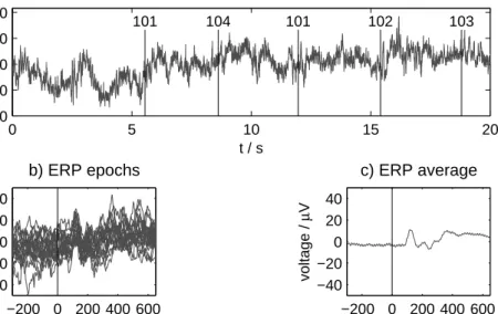
0 5 10 15 20 0 30 60 90 120 101 104 101 102 103 t / s voltage / µ V

a) continuous EEG record

−200 0 200 400 600 −40 −20 0 20 40 t / ms voltage / µ V b) ERP epochs −200 0 200 400 600 −40 −20 0 20 40 t / ms voltage / µ V c) ERP average

Figure 2.6:Event-related potentials and the ERP average. a) A section of a con-tinuous EEG record at one electrode (OZ). The vertical lines with numerical codes mark the presentation times of different types of stimuli. b) Superimposition of 20 epochs corresponding to one of the stimuli (101) for pre- and poststimulus inter-vals of lengthsTpre=300 ms andTpost=650 ms. c) Average of 177 epochs. The ERP response is starting about 100 ms after stimulus presentation.

To investigate ERPs, a stimulus or a set of stimuli that are equivalent in a certain respect is repeatedly presented to a subject, and the sections of the EEG record around the time of the stimulus presentation, the so-called epochs, are cut out and collected into an ensemble. Ifx(t) is the EEG time series andti(i=1. . .n) are the

presentation times of a stimulus, then

xi(t)=x(ti+t) for −Tpre≤t≤Tpost (2.1)

is theith epoch for the given lengths of the pre- and poststimulus interval. (In the case of several EEG channelsx is to be taken as a vector whose components correspond to the electrodes.) The common method to analyze the epoched data is to calculate the mean over stimulus presentations,

¯ x(t)= 1 n n

∑

i=1 xi(t), (2.2)

and to interpret the time course of the result (Fig. 2.6).1 _{Specific features of this}

time course that can be associated with physiological or cognitive processes are called ERP components (see below).

There seems to be no exact, generally accepted definition of the term event-related potential (cf. Lopes da Silva, 1998b). In the common use especially in stud-ies interpreting the epoch average, the mean ¯x(t) is looked at astheevent-related potential, and it is more or less implicitly interpreted as a signal that is generated by a neuron population specifically activated in the processing of the given stimu-lus, and that is superimposed onto an unchanged “ongoing background EEG” re-garded as noise. In this view, the averaging method is just a straightforward way to

1_{To compensate for drifts and to prepare the ERP average for comparison between conditions (see}

below), it is common to additionally perform a “baseline correction”: The time average of the mean over the prestimulus interval is subtracted: ¯x(t)−R0

(21)

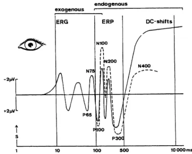
Figure 2.7:Schematic time course of averaged event-related responses to visual stimuli. ERP components are differentiated into exogenous and endogenous, the latter including the N100, P300, and N400 (see text). Longer lasting voltage changes are referred to as DC-shifts (direct current shifts). Note the inverted verti-cal sverti-cale plotting negative voltage to the top, which is customary in ERP research. Reproduced with permission from Altenm ¨uller and Gerloff (1998), Psychophysiol-ogy and the EEG, Fig. 32.1 A. In Niedermeyer and Lopes da Silva, editors, Electro-encephalography: Basic Principles, Clinical Applications, and Related Fields. Copyright

c

1998 Lippincott Williams & Wilkins.

increase the signal-to-noise ratio of the ERP measurement. Other authors assume that event-related potentials are not just an independent addition to a background EEG, but the result of a transient reorganization of the ongoing activity.2Lopes da Silva (1998b) tries to reflect this controversy in his concept of ERPs as slight EEG changes that are related to a particular event. Though this definition is fairly gen-eral, it, too, implicitly refers to an analysis procedure that distinguishes between those changes and some normal state the changes are related to.

A neutral alternative is to consider as an event-related potential just the en-semble of epochs, that is the collection of voltage (potential) recordings that are temporally related to a given event. In the language of statistical time series analy-sis, the processing of the EEG record to generate epoch ensembles corresponds to the definition of a stochastic processX(t), and each epochxi(t) constitutes a

reali-zation of this process. As such, the ensemble of realireali-zations is open to a multitude of different data analysis approaches. In this view, the calculation of the ensemble average is just the most basic statistical evaluation that can be applied, the statisti-cal moment of first order. This and any other descriptive statistic can be connected with certain theoretical assumptions, or it can simply be looked at as an empirical quantity that may be correlated with experimental variations. Therefore, even if the common ERP theory of an invariant signal embedded in random noise would prove not to be valid, the findings regarding ERP components would still be valu-able.

As noted above, the ERP average exhibits characteristic wave forms (with am-plitudes in the range from 2 to 20µV) that have been shown to correlate with

cer-2_{Makeig et al. (2002) present results indicating that ERPs are generated by phase-resetting of}

(22)

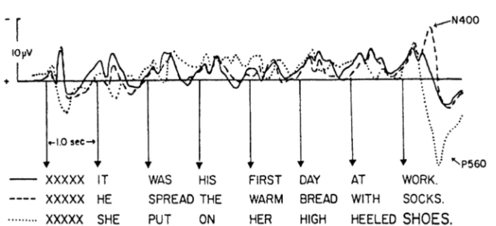
Figure 2.8:The N400 component in the experiment of Kutas and Hillyard. The graph shows the ERP average for the three experimental conditions that are illus-trated with a sample sentence below. The presentation of a semantically incongru-ent noun at the end (dashed line) elicits a negativity around 400 ms compared to a noun that makes sense (continuous line). In the third condition, the noun at the end is semantically congruent but physically deviant (printed in a larger font, dot-ted line); this elicits a late positivity (“P560”). Reproduced with permission from Kutas and Hillyard (1980b), Reading senseless sentences: Brain potentials reflect semantic incongruity.Science, 207. Copyright c1980 AAAS.

tain physiological or cognitive processes (Fig. 2.7).3 _{ERP components can be}

differ-entiated into “exogenous” and “endogenous”, where the former depend directly on physical properties of the stimulus while the latter are determined by psycho-logical variables and therefore are related to cognitive processes. Exogenous ERP components generally occur up to ca. 100 ms after stimulus presentation, endoge-nous components after this point. Components are normally named following their polarity (N for negative, P for positive) and their approximate latency, that is the delay of their occurrence relative to the presentation of the stimulus, but they are also distinguished according to their topography (distribution over the scalp) and morphology (shape of the waveform).

The earliest endogenous ERP component is the N100, a negativity with a la-tency of about 90 to 200 ms. It corresponds to an initial “orienting” response that is the reaction to an unexpected stimulus. The N100 habituates (that is, its amplitude gets smaller over time during an experiment) and it is modulated by the selective attention of the subject. An N100 follows not only the onset but also the offset of a stimulus.

The P300 is the most prominent ERP component. Its latency lies between 280 and 700 ms such that probably the P300 actually consists of a general “late positive complex” of subcomponents. Its common (“oddball”) paradigm is the infrequent presentation of one stimulus embedded in a sequence of many presentations of another stimulus. If the subject attends to the stimuli, the infrequent one elicits a P300 component whose amplitude is inversely related to the stimulus probability. An important language-related component is the N400 that has originally been found by Kutas and Hillyard (1980b,a). They presented sentences to their subjects, word by word with an interstimulus interval of 1 s. In some of the sentences, the last word was semantically incongruent, that is it did not make sense in the given context. In this case, the ERP response to the last word shows a strong negativity around 400 ms after stimulus presentation compared to a sentence ending with a semantically appropriate word (Fig. 2.8). The N400 has since been demonstrated to show up not only in response to incongruent words, but to reflect a low

(23)

gree of semantic expectancy in general. It can be elicited by printed, spoken, as well as sign language and occurs not only with words in sentences, but also in a so-called priming paradigm, where a single word presented first provides the se-mantic context for a second one (cf. Altenm ¨uller and Gerloff, 1998). Though it is an ERP component specific to language, which is generally associated with areas in the left hemisphere of the brain, the N400 shows no preponderance on the left but is broadly distributed temporoparietally4_{on both sides (Friederici, 1995).}

In the description of the N400 component, a detail has already been mentioned that is generally important in the utilization of ERP averages and other quanti-ties for the purposes of cognitive science. Up to now, ERP components have been presented as absolute responses to a given stimulus. But in the context of the expe-riment of Kutas and Hillyard (1980b), the response to the semantically incongruent noun can only be interpreted in comparison to the response to a noun that fits into the sentence. That means the N400 observed here is arelativenegativity.

Generally speaking, each trial of an experiment—the presentation of a stimu-lus or a sequence of presentations that form a unit, like the parts of a sentence— belongs to one of the so-called conditions of an experiment. These experimen-tal conditions correspond each to a different stimulus (in the simplest case) or to classes of stimuli that are equivalent in a certain respect within each group and define certain variations between groups. EEG epochs are sorted into ensembles according to the experimental condition of the trial, and the average ERP (or other quantities) are calculated for each condition separately. Important for the inter-pretation of the experimental results is then thedifferencein the stimulus response for the different experimental conditions that is caused by a small variation of the stimulus class.5 _{This difference can be quantified on a generic scale by relating it}

to the variation over trials or over subjects, determining its statistical strength. The reason for this approach is that the ERP response to a set of stimuli pre-sented in an experiment does not solely correspond to those specific aspects that the experimenter has in mind, but includes a manifold of operations necessary for stimulus processing as well as the “background” activity of the brain that is not related to the stimulus at all. Part of this may be reduced by the averaging tech-nique or other statistical procedures, diminishing the impact of random influences or of the individual features of a stimulus belonging to a class. But still much of the remaining activity is related to stimulus processing in general, for instance char-acter recognition or retrieval of lexical information. These processes are common to all experimental conditions, and so the part corresponding to their experimen-tally relevant aspects can only be filtered out by comparing the responses in the conditions.

The experiment of Kutas and Hillyard defines three experimental conditions, the first containing normal sentences ending with a semantically appropriate noun, the second sentences with a semantic incongruity, and a third group of sentences with a noun that fits in but is shown in a larger font (Fig. 2.8). Looking at the ERP average elicited by the terminal noun (the so-called critical item) in the second con-dition (dashed line), there is an early negative peak that can be labeled as an N100 component, but that is apparently not related to the semantic incongruity because it shows up in almost exactly the same form in the control condition (continuous line). The N400 component observed here is therefore to be taken as the negativity of the average in the “semantic incongruity” experimental condition relative to the average in the control condition.

As noted above, event-related potentials may be conceptualized as stochastic

4_{For an explanation of this and related terms used to describe the topography of ERP components,}

see Fig. 2.5.

5_{See Coles and Rugg (1995). Analogous considerations are valid for the cognitive sciences in general;}

(24)

processes, the epoch ensembles being samples of realizations. The ERP average is the traditionally most important statistic of the process used in its analysis, and accordingly there is a large number of studies presenting averages in different ex-perimental contexts, defining ERP components and associating them with brain processes. Nonetheless, the mean is just one of the moments of a stochastic pro-cess and there are other statistics possibly illuminating different aspects of brain dynamics. Some of these have been employed in ERP analysis for quite some time, most notably the calculation of event-related nonstationary band power, determin-ing effects of so-called event-related desynchronization and synchronization (ERS / ERD, cf. Pfurtscheller, 1998; Altenm ¨uller and Gerloff, 1998). Despite their name, these effects do not refer to the observation of synchronization processes in the strict sense. Their labels are based on the notion that changes in band power at a single electrode are caused by variations in the strength of local synchronization in the neuron population subserving it, generating a stronger or weaker collective effect at the scalp.

More recent alternative evaluation methods of ERPs are inspired by concepts of nonlinear dynamics, like the approach of beim Graben (2001), who encodes ERP epochs into symbol strings and applies entropy measures of complexity to determine the symbolic dynamics of ERPs (see also beim Graben et al., 2000). In a similar way, the subject matter of the present work is to apply the theory of phase synchronization to event-related potentials. Here, instead of calculating the mean of voltages, event-related phase synchronization is analyzed by computing the frequency-specific instantaneous phase of ERP epochs (Sec. 3.2) and quantify-ing the peakedness of the distribution of the phase difference between electrodes as a measure of the statistical strength of phase synchronization (Sec. 3.3). The physical theory underlying this approach will be introduced in the next section.

2.3 Phase synchronization

Synchronization is a subject of physics with a long tradition, going back to its dis-covery by Huygens in 1665. It is an essentially nonlinear phenomenon that can be observed in a multitude of technical as well as natural systems, including the human brain. The presentation in this section follows the monograph by Pikovsky et al. (2001). It is aimed at the notion of phase synchronization as the reference point of the analyses presented in this work.

In general terms, synchronization is the adjustment of the rhythms of self-sustained oscillators due to coupling. A self-self-sustained oscillator is a dynamical system that generates oscillations out of itself, rather than adhering to an externally provided rhythm. A classic example of a periodic self-sustained oscillator is the pendulum clock. It possesses an internal energy reservoir in the form of weights and uses that energy to generate the periodic motion of its pendulum. Amplitude and frequency of this oscillation are specific properties of the clock mechanism and as such are constant within certain bounds.

In the theoretical description, a periodic oscillator corresponds to thelimit cycle of a nonlinear dynamical system (cf. Pikovsky et al., 2001, Ch. 7). Combining the different variables describing the system state into a vector~x, the dynamics of a system can generally be described by the differential equation ˙~x = ~f(~x). If this equation possesses a periodic solution with periodT0,

~

x0(t)=~x0(t+T0),

that attracts neighboring system states, this solution is called a limit cycle (Fig. 2.9). Thephaseφof the oscillator is a coordinate along the limit cycle (a function of~x)

(25)

2.3 Phase synchronization 25

x 1 x

2

Figure 2.9:The limit cycle (black) of a two-dimensional dynamical system (~x=

(x1,x2)). Neighboring trajectories (gray lines) approach the cycle and join the peri-odic motion along it.

φ = 0 π/2 π 3/2π 2π→ 0 π/2 t x 2 x 1 x 2 0 π/2 π 3/2π φ

Figure 2.10:The phase on a circle-shaped limit cycle with uniform motion is the angle between a fixed direction (e.g. positivex1axis) and the current system state (•). The motion on the circle corresponds to a sinusoidal time series. Periodically recurring system states (•connected with dashed line) are assigned the same value of the circular phase by resetting it after increasing with time over a period of 2π.

whose value is uniformly increasing with time, gaining 2πwith every oscillation:

˙

φ=const.=ω0, where ω0=

2π

T0

. (2.3)

The constant derivative of the phaseω0is called the natural frequency of the

oscil-lator.6 _{In the simplest case of a circle-shaped limit cycle with uniform motion the}

phase is the angle within the circle between the current system state and an arbi-trary reference direction (Fig. 2.10). The complementary coordinate in the radial direction is called amplitude.

In the notion of phase that has just been established there is an ambiguity. On the one hand, the phase is an ever-increasing variable that describes the continuing oscillations on the limit cycle. With every oscillation the phase gains 2π, such that the integral part ofφ/2πcan be seen as the number of full oscillations the system has performed. This may be called the linear aspect of the phase. On the other hand, the motion described by the phase is periodic, and the system states of a periodic oscillator corresponding to phasesφ,φ+2π,φ+4π, . . . are physically identical so that these values are equivalent. In this respect, calculations and com-parisons concerning the phase have to be taken modulo 2π. (The circular aspect

6_{Normally, the quantity}_f ₌₁_/_T_(where_T_{is the period) is called the frequency of an oscillation.}

In this and the following methodological sections, by the term frequency the author is referring to the

(26)

of the phase.) Since consecutive intervals of length 2π are equivalent, it is often convenient to wrap the linear phase into one of these intervals, e.g. [0,2π[ (the fractional part of φ/2π) or [−π, π[. In the following, the linear and the circular interpretation of phase (including phase differences) will not be distinguished ex-plicitly as long as the relevant aspect can be concluded from the context. With time series, a linear phase can be reconstructed from the circular phase by “unwrap-ping”, i.e. shifting the phase time series by 2πat each discontinuity.

Because the limit cycle is stable, deviations from it in the radial direction will be compensated quickly, while modifications of the phase will be retained. Therefore, if the periodic oscillator is subjected to a small external force ~p of strengththat depends on the system state and varies with time,

˙

~x=~f(~x)+ ~p(~x,t),

this force will mainly affect the phase. Because the amplitude remains unchanged, the modified dynamics of the system can be described in terms of phase only:

˙

φ=ω0+Q(φ,t), (2.4)

whereQrepresents the effect of the force on the phase.

Two self-sustained oscillators A and B can be bidirectionally coupled if each of them exerts a force on the other one. Since the time dependence of these forces bears on the respective oscillator’s phase, the dynamics of phasesφA,Bcan be

writ-ten as

˙

φA=ωA+QA(φA, φB), φ˙B=ωB+QB(φB, φA),

whereωA,Bare the natural frequencies of the uncoupled oscillators (corresponding

to=0) and the functions QA,B represent the coupling forces. These equations

can be further simplified if the natural frequencies are close to each other,ωA≈ωB.

Approximating by time-averaging over fast variations in the coupling forces one retains only the resonant terms in the Fourier expansion ofQA,B(cf. Pikovsky et al.,

2001, Ch. 7 & 8). As a result, the phase dynamics depends on the difference of the oscillator phases only:

˙

φA=ωA+qA(φA−φB), φ˙B=ωB+qB(φB−φA).

Introducing thephase difference∆φ=φB−φAas a new variable, its dynamics can

be described by

˙

∆φ=∆ω+q(∆φ), (2.5) where∆ω=ωB−ωAis the difference between the natural frequencies (the

“detun-ing”) andq(∆φ)=qB(∆φ)−qA(−∆φ) is the coupling function that is 2π-periodic in

∆φ.7 _{This is the basic equation describing the phenomenon of bivariate}

synchro-nization which is further analyzed in the following.

Synchronization sets in if the frequency detuning is not too large or the cou-pling is strong enough. If the extremal values ofq(∆φ) are denoted byqmin,max, the

synchronization condition is given by the inequality

−qmax<∆ω <−qmin, (2.6)

defining a triangular synchronization region in the space of parameters (,∆ω). In this case, the dynamics of the phase difference has a stable fixed point∆φs and

after a transition time the phase difference stays constant:

∆φ→∆φs=const., φB=φA+∆φs.

7_{Synchronization is also possible if the natural frequencies are close to a rational ratio different}

from 1:ω_A/ω_B≈m/n, wherem,n∈N. In this case ofm:nsynchronization Eq. 2.5 still holds with

∆φ=mφB−nφA,∆ω=mωB−nωA, andq(∆φ)=mqB(∆φ)−nqA(−∆φ).

Equation 2.5 also holds for the phase difference between an oscillator (B) and an external periodic force (A) acting onto it. This can be seen as an extreme case of asymmetric coupling,qA=0.

(27)

2.3 Phase synchronization 27 0 50 100 150 200 250 300 350 400 −50 0 50 100 150 200 ∆φ t / ε−1

Figure 2.11: Dynamics of the phase difference with the couplingq(∆φ)=−sin(∆φ) for different frequency detunings ∆ω= −1.001, 0, 1.01, 1.1 (from bottom to top). In the synchronized regime |∆ω| ≤the phase difference is constant. Close to the synchronization transition it is nearly constant for most of the time, interrupted by phase slips ±2π occurring with a constant period (here T∆φ ≈ 140,∞, 44.3,13.7−1_{, corresp.). Time is given in units of}−1_{, frequency in units}

of. After Pikovsky et al. (2001), Fig. 7.5.

Here, synchronization manifests itself in a fixed relation of the two oscillator pha-ses, a phenomenon that is calledphase locking. The rhythms of the oscillators are perfectly adjusted to each other, implying that their instantaneous frequencies are identical, the so-calledfrequency entrainmentφ˙B=φ˙A.

This is an idealized result due to the approximations that were made in the derivation of the phase difference dynamics. In general in the synchronized regime the phase difference is not constant but performs small oscillations around a con-stant value. The phases are not exactly locked to each other, but still the phase difference isboundedwithin one oscillation cycle:

∆φmin≤∆φ≤∆φmax with ∆φmax−∆φmin<2π (2.7)

(cf. Rosenblum et al., 1996). Though in this case the instantaneous frequencies ˙

φA,B are not identical, the condition of frequency entrainment still holds for

time-averaged frequencies,

ΩB=ΩA with ΩA,B=lim

t→∞

φA,B(t)−φA,B(0)

t , (2.8)

because the contribution of the oscillating phase difference vanishes in the limit. If the synchronization condition (Eq. 2.6) is not met, the phase difference in-creases (or dein-creases) all the time. Close to the transition to synchronization it stays almost constant for long periods of time, but then performs a full cycle rather quickly, gaining (or losing) 2π. Thesephase slips(Fig. 2.11) occur regularly, giving rise to a difference of the average oscillator frequencies of

∆Ω=ΩB−ΩA= 2π T∆φ , where T∆φ= Z 2π 0 d∆φ ∆ω+q(∆φ)

(28)

−1 0 1 0 0.5 1 −1 0 1 ∆ω ε ∆Ω

Figure 2.12:The synchronization diagram shows the difference of the average fre-quencies∆Ωas a function of the coupling strengthand the frequency detuning

∆ω. If the oscillators are not coupled (=0) the average frequency difference is

just the detuning,∆Ω=∆ω. For larger coupling strength >0, the range of de-tunings for which synchronization is achieved (frequency entrainment,∆Ω=0) increases linearly, forming the triangular synchronization region. In the unsyn-chronized state,∆Ωis different from zero but still smaller than∆ω. The diagram was calculated for sine coupling,q(∆φ)=−sin(∆φ).

is the fixed period of the phase slips. Close to the transition points at ∆ωc = −qmin,maxthe average frequency difference depends on the difference of the

nat-ural frequencies according to

∆Ω∼₌_±q_|_∆_ω2₋∆_ω2 c|.

The full dependence of∆Ωon and∆ω including the synchronization region is depicted in Fig. 2.12 for the case of sine coupling.

Up to this point, synchronization has been considered in the case of determin-istic periodic oscillators only. In contrast, most natural systems are exposed to irregular external perturbations. The straightforward way to include such influ-ences in the model is to add a noise term to the phase difference dynamics (cf. Pikovsky et al., 2001, Ch. 9):

˙

∆φ=∆ω+q(∆φ)+ξ(t), (2.9) whereξ represents mean-free noise (hξ(t)i=0). By this, Eq. 2.5 is turned into a Langevin equation describing a stochastic process. Now, in addition to the fre-quency detuning, the coupling has also to overcome the effect of the noise to achieve synchronization. If the noise is strong enough, it can drive the phase dif-ference out of one cycle into the next one, causing a sequence of irregular phase slips. The phase difference is then performing a random walk from cycle to cycle, that is biased into one direction if the detuning is different from zero (Fig. 2.13a). For unbounded noise this is possible (with a small probability) even for arbitrar-ily high coupling strengths. In this case the phase difference is not bounded, and synchronization in the sense that has been introduced above (Eq. 2.7) can not be achieved. Still the coupling has an effect on the phase difference dynamics that

(29)

2.3 Phase synchronization 29 0 200 400 600 800 1000 t −30 −20 −10 0 10 ∆φ/2π a ) b ) c ) d ) 3 −π 0 π ∆φ 1 2

Figure 2.13:The dynamics of the phase difference of coupled noisy oscillators. a) The linear phase difference performing a random walk. 1: The oscillators are uncoupled. 2: Coupled oscillators with small noise and moderate frequency mis-match; there are rare phase slips of−2π. 3: Stronger noise than for curve 2, phase slips are occurring frequently. b)–d) Histograms of the circular phase difference, corresponding to curves 1–3. In the uncoupled case the distribution is uniform. Stronger noise is smoothing out the peak caused by coupling. Reproduced with permission from Pikovsky et al. (2001),Synchronization: A Universal Concept in Non-linear Sciences, Fig. 9.2. Copyright c2001 Cambridge University Press.

can be recognized in the probability distribution of the circular phase difference (Fig. 2.13b–d). In Sec. 3.3, this effect will be used to introduce a statistical measure of synchronization strength as an alternative to the strict definition.

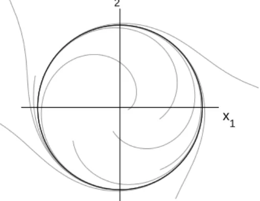
Not only noisy, but also chaotic oscillators can be synchronized (cf. Pikovsky et al., 2001, Ch. 10). The main issue in this case is to obtain a suitable definition of the phase of such a system. A common example of a chaotic oscillator is the R ¨ossler system (Fig. 2.14). Here, in place of a limit cycle we find a tangle of trajec-tories forming the chaotic attractor. Though in the projection onto the x,y-plane it resembles a smeared circle-shaped limit cycle, in this case it is not possible to introduce a variable in the state space that is uniformly increasing with time. Still, there are a number of different methods to calculate a quantity whose properties are close to that of the phase of a periodic oscillator and that can be utilized to analyze chaotic synchronization; some of them are discussed in greater detail in Sec. 3.2. A simple approach is to define

φ=arctany

x and A=

q

x2₊_y2_, _(2.10)

that is, to take the angle8 _{around the origin in the projection plane as the phase,}

and correspondingly the distance from the origin as the instantaneous amplitude A.

An important phenomenon of chaotic synchronization can be observed with

8_{The arctan is the common formulation of this definition, though this function only gives values in}

the range [−π 2;

π

2[. To obtain the full circular phase, one should useφ=arg(x+iy) or the equivalent

(30)

x y z −10 0 10 20 −20 −10 0 10 x y

Figure 2.14:The attractor of the R ¨ossler oscillator for standard values of the pa-rameters (Eqs. 2.11). The right panel is showing the projection onto thex,y-plane. The angle between the positivexaxis and a particular system state (•) is indicated, which is one possible definition of the phase of this chaotic oscillator.

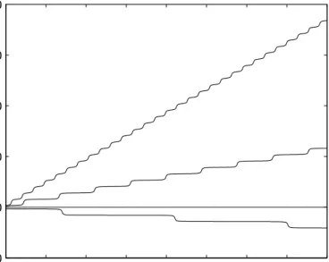
a) 0 500 1000 1500 2000 time −10 10 30 50 70 φ1 −φ2 C=0.01 C=0.027 C=0.035 b) 5 9 13 17 A₁ 5 9 13 17 A2

Figure 2.15:Phase synchronization of coupled R ¨ossler oscillators (Eqs. 2.11 with ω1,2=1±0.015). a) The phase differenceφ1−φ2of the oscillators over time. For coupling strengthC=0.035 there are no phase slips. b) In the synchronized regime the amplitudesA1,A2 remain chaotic and are almost uncorrelated. Reproduced with permission from Rosenblum et al. (1996), Phase synchronization of chaotic oscillators.Physical Review Letters, 76, Fig. 1. Copyright c1996 American Physical Society.