Intangible assets and capital structure
Steve C. Lim, Texas Christian UniversityAntonio J. Macias, Baylor University Thomas Moeller, Texas Christian University
August 2014
Abstract
Tangible assets, many of which can be easily collateralized, support debt. Accordingly, the amount of tangible assets is well-established as a principal driver of leverage. As investing is shifting more and more from tangible to intangible assets, it becomes crucial to understand to what extent intangible assets support debt. Analyzing this question empirically has been largely unfeasible due to the lack of information about firms’ self-created intangible assets. We take advantage of a recent accounting rule change that allows us to observe market-based valuations of identifiable intangible assets of firms that are acquired. In these firms, both tangible and intangible assets are positively related to leverage. Intangible assets have the strongest effect on leverage in technology firms and in firms with low tangible asset intensity. On a per dollar basis, intangible assets support approximately half as much debt as tangible assets.
Key words: Capital structure, leverage, intangible assets
We thank Houlihan Lokey for providing the M&A purchase price allocation data. Antonio Macias and Thomas Moeller wish to thank the Neeley Summer Research Awards program and the Luther King Capital Management Center for Financial Studies in the Neeley School of Business at TCU for their financial support for this research. All errors are our own.
Contact information:
Steve C. Lim, TCU Box 298530, Fort Worth, TX 76129, [email protected], 817.257.7536.
Antonio J. Macias, One Bear Place #98004, Waco, TX 76129, [email protected], 765.412.6397. Thomas Moeller, TCU Box 298530, Fort Worth, TX 76129, [email protected], 817.760.0050.
1
“The big difference between the new economy and the old is the changed nature of investment. In the past, businesses primarily invested in the tangible means of production, things like
buildings and machines. The value of a company was at least somewhat related to the value of its physical capital; to grow bigger, a business had to build new factories roughly in proportion to the increase in its sales. But now businesses increasingly invest in intangibles. And once you’ve designed a chip, or written the code for a new operating system, no further investment is needed to ship the product to yet another customer.” (Paul Krugman, New York Times, 22 October 2000) I. Introduction
Firms with more tangible assets tend to have more debt (e.g., Harris and Raviv, 1991; Frank and Goyal, 2008; Parsons and Titman, 2009). This relation is not surprising because many tangible assets constitute suitable collateral. They can be redeployed at relatively low transaction costs when the borrower becomes distressed or defaults. Therefore, borrowing costs should be relatively low when firms’ tangible assets support their debt, resulting in a positive relation between asset tangibility and financial leverage.
Campello and Giambona (2013) take the relation between asset tangibility and capital structure one step further and argue that it is not only the tangibility of assets that increases debt capacity, but also the ease with which tangible assets can be sold. For example, it should be much easier to sell standard equipment compared to specialized equipment. Their paper offers a refinement of the traditional focus on tangible assets. Several theoretical models also predict that higher asset liquidity should increase the optimal leverage (e.g. Shleifer and Vishny, 1992; Morellec, 2001).
We expand the empirical capital structure literature by examining how firms’ intangible assets affect leverage. On the one hand, collateralizing intangible assets is more challenging. Compared to tangible assets, intangible assets tend to be more difficult to identify, separate, utilize, and value. Furthermore, their value is more sensitive to who owns and employs them. These features make many intangible assets poor collateral and favor financing with equity instead of debt, leading to a negative relation between intangible assets and leverage.
2
On the other hand, assets can support debt not only because they are useful collateral, but also because they enable the firm to be profitable and generate cash. As the Paul Krugman quote above implies, many intangible assets can very effectively generate cash, frequently more so than tangible assets. Intangible assets that generate substantial cash should be well-suited to support debt, allowing a positive relation between intangible assets and leverage. Furthermore, Loumioti (2012) reports that lenders accept liquid and redeployable intangible assets as collateral because they have found innovative ways of leveraging, financing, and valuing intangible assets. Ellis and Jarboe (2010) provide examples of such intangible asset-backed loans.
Because intangible assets play an increasingly important role in today’s knowledge-based economy, it is important to investigate the impact of intangible assets on capital structure choices with empirical data. Nakamura (2001, 2003) estimates that the annual investment rate in intangible assets in the U.S. is $1 trillion as of 2001, practically equal to that in tangible assets. Furthermore, a third of the value of U.S. corporate assets are intangible assets according to Nakamura’s analysis.
Accounting rules distinguish between two types of intangible assets, acquired and self-created. A major obstacle to empirically studying the relation between intangible assets and capital structure is that the value of a firm’s self-created intangible assets is largely unobservable. Due to the conservatism tradition in accounting, self-created intangible assets are left off the balance sheet and are not reported in any of the financial statements or regulatory filings. Only intangible assets that were acquired through external transactions, such as mergers and acquisitions, are reported on balance sheets. The unreported self-created intangible assets should be substantial for many firms. Examples of such intangible assets include Apple’s operating systems iOS and OSX, Microsoft’s Windows and Office software, Coca-Cola’s Coke brand name, and American Express’ list of customers’ identities, spending patterns, and creditworthiness.
3
We get around this data limitation with a unique dataset that takes advantage of a recent accounting rule change that requires an acquiring firm to provide detailed market value estimates of the target firm’s identifiable intangible assets. Starting in July 2001, Statement of Financial Accounting Standards (SFAS) 141 requires that an acquiring firm allocates the purchase price paid for a target to identifiable assets, both tangible and intangible, based on estimated fair market values at the time of the acquisition, before allocating the remaining purchase price to goodwill.1 These estimates of the market values of the tangible and intangible assets are reported in the acquirers’ 10-Ks or 10-Qs where we, with the generous help of Houlihan Lokey, obtain them. In effect, SFAS 141 provides the fair market values of target firms’ self-created identifiable intangible assets that are based on arm’s length transactions. Prior to SFAS 141, acquirers generally allocated the majority of the purchase price to acquisition goodwill without providing valuations of identifiable intangible assets.
Our dataset contains 429 publicly traded non-financial U.S. target firms that were acquired by publicly traded U.S. firms between 2002 and 2011. The major drawback of our novel data is that it only gives us a snapshot on the fair market values of targets’ tangible and intangible assets at the time of their acquisitions. We assume that there are no systematic changes in the values of these assets in the year prior to the acquisitions. With this assumption, we then examine the relation between targets’ tangible and intangible assets, measured at the time of the acquisition, and the targets’ leverage, measured at the last fiscal year-end before the acquisition.
1Financial Accounting Standards Board (FASB) standards are now incorporated into FASB’s Accounting Standards
Codification (ASC) and SFAS 141 can be found under FASB ASC 805: Business Combinations. However, to be consistent with prior literature, we will refer to SFAS 141 instead of ASC 805. FASB revised SFAS 141 in 2007 and it is now called SFAS 141R. Paragraph 14 of SFAS 141R states that “The acquirer’s application of the recognition principle and conditions may result in recognizing some assets and liabilities that the acquiree [target] had not previously recognized as assets and liabilities in its financial statements. For example, the acquirer recognizes the acquired identifiable intangible assets, such as a brand name, a patent, or a customer relationship, that the acquiree [target] did not recognize as assets in its financial statements because it developed them internally and charged the related costs to expense.”
4
While asset values generally change over the year before an acquisition, and such value changes can even be the reasons for some acquisitions, if the changes are not systematic, they should mainly add noise to our estimations. Firms that become targets and are eventually acquired may have unique unobservable characteristics that drive intangibles to be positively correlated to leverage. We try to control for such biases that are created by systematic changes in asset values and the endogeneity of becoming a target.
We find that targets’ intangible assets are positively related to targets’ pre-acquisition leverage, suggesting that intangible assets support debt in similar ways as tangible assets do. Our results are robust to using Heckman specification models to address potential sample-selection endogeneity concerns. In terms of the quantitative impact of intangible assets, the coefficient estimates of intangible assets are similar to those on tangible assets in our leverage regressions. When we examine the dollar effect of assets on debt, each dollar of tangible assets supports about $0.17 of debt while each dollar of intangible assets supports on average $0.09 of debt.
While our dataset is limited, there are no good alternatives for measuring the value of firms’ self-created intangible assets. A possible estimate would be the difference between the market value of the firm and the book value of assets. Yet, it is unclear whether such an estimate measures the value of intangible assets, the difference between the market and book values of tangible assets, or the firm’s future growth potential. Furthermore, this variable is mechanically tied to market leverage and therefore not useful in examining the market leverage. Despite the limited dataset, we consider it unlikely that our findings only apply to the firms in our distinct sample.
We also examine the effects on leverage of components of intangible assets. Under SFAS 141, acquirers allocate the purchase price to two main categories, tangible and intangible assets. The intangible assets category is further divided into five categories of identifiable intangible assets and one category of unidentifiable intangible assets, i.e., acquisition goodwill. Among the
5
identifiable intangible asset categories, two are technology-related: 1) developed technology, including patents, and 2) in-process research and development. Another two are marketing-related: 1) trademarks and trade names, including domain names, and 2) customer-related assets, including backlog, customer contracts, and customer relationships. The final category covers all other identifiable intangible assets.
Technology-related and other intangible assets have the largest impact on leverage. Not surprisingly, we find that technology-related intangible assets have the strongest effect on leverage in technology firms. In addition, we find that the intangible assets have more significant effects on debt financing in firms with low tangible asset intensity, i.e., firms with low ratios of tangible assets to firm value.
We contribute to the capital structure literature by identifying intangible assets as important determinants of firms’ capital structures. Compared to tangible assets, each dollar of intangible assets supports approximately half the amount of debt, on average. This effect is substantial and can lead to problematic biases when it is ignored in empirical capital structure studies. Our study also further validates the usefulness of the SFAS 141-based purchase price allocation data that other papers have demonstrated. For example, Kimbrough (2007) offers evidence that the value of intangible assets reported in the purchase price allocation provides valuable information to equity investors.
II. Hypotheses
Prior studies largely ignore intangible assets as determinants of leverage because the values of firms’ intangible assets are largely unobservable. Furthermore, repossessing intangibles in case of default or bankruptcy is difficult compared to most tangible assets, and agency problems can prevent the efficient use of intangible assets in production processes by anyone other than the owners of the intangible assets (Rampini and Viswanathan, 2013).
6
We develop our hypotheses in the context of a standard leverage (Lev) regression model, such as Campello and Giambona (2013):
, , , , 1 1 , N T i t i t i t i t i t i t
Lev α βTan γCon δ Firm λ Year ε
= =
= + + +
∑
+∑
+ (1)where Lev is the long-term debt divided by total assets, Tan stands for the ratio of tangible assets to total assets, Con is a vector of control variables, Firm is a firm fixed effect, Year is a year fixed effect, i denotes a firm, and t denotes a year.
We add intangible assets as an additional independent variable to this standard specification. Since the fair market value of self-created intangible assets is available only at the time when the target is acquired, the purchase price allocation data limits us to a cross-sectional analysis. Consequently, we remove the firm fixed effects. Due to our relatively short sample period, we also do not include year fixed-effects. Therefore, our main regression specification is:
, , , , ,,
i t i t i t i t i t
Lev =α β+ Tan +ωInt +γCon +ε (2)
where Int stands for the fair market value of intangible assets reported in the purchase price allocation data of the bidding firms’ 10-Ks or 10-Qs, normalized by the purchase price.
Our null hypothesis is that the fair market value of intangible assets does not affect leverage, i.e., ω=0. Alternatively, intangible assets can affect leverage the same way as tangible assets do, implying ω>0. A third possibility is that firms that create substantial amounts of intangibles are particularly sensitive to the negative effects of debt and therefore use particularly low leverage, implying ω<0.
We also separately examine the effects on leverage of the three components of identifiable intangible assets (technology-related, marketing-related, and other). Specific components that matter when they should matter are further evidence that the leverage results are indeed caused by the intangible assets. First, intangible assets that are most relevant for a specific industry should
7
have larger effects on leverage in that industry. We test this conjecture by examining whether technology-related intangible assets matter more for firms in technology industries than firms in other industries. Second, intangible assets should matter less for firms that have high tangible asset intensities, i.e., firms where tangible assets comprise large portions of the firms’ values. We test this conjecture by running our regressions separately for firms with high and low tangible asset intensities.
III. Data
The sample comprises 429 U.S. public firms that became targets of completed acquisitions by U.S. public acquirers between 2002 and 2011. Houlihan Lokey provides us the original dataset of 4,652 acquisitions with purchase price allocation (PPA) information that is hand-collected from 10-Ks and 10-Qs.2 We match the 4,652 targets with Compustat using target company names. This matching reduces the sample to 1,089 targets. Limited data availability in Compustat and the exclusion of subsidiary and foreign targets reduce the sample size to 553 firms.3 After excluding financial firms, our final sample consists of 429 firms.
Appendix A shows how the disclosure formats of the purchase price allocations in their 10-K filings to the Securities and Exchange Commission differ between two firms in our final sample. These variations in the reporting formats make collecting the purchase price allocation data nontrivial. Figure 1 shows the composition of purchase price allocations. It is a modified copy from the Houlihan and Lokey 2011 Purchase Price Allocation Study. The first example in
2 Houlihan Lokey is a privately-held global investment banking firm founded in 1972. The firm operates through
three main service lines: corporate finance (comprising mergers and acquisitions, capital markets, and second advisory), financial restructuring, and financial advisory services. For 2012, Houlihan Lokey ranked No. 1 in announced U.S M&A deal volume for deals under $3 billion.
3 We exclude from our sample 50 observations where the total purchase price allocation is less than half of the
target’s book or market value of assets at the time of the last fiscal year-end of the target. A -50% offer premium suggests a severely distressed target. For such targets, our assumption of no substantial change in the target’s business situation between the prior fiscal year-end and the acquisition date is almost certainly violated.
Furthermore, the -50% threshold can capture subsidiary or comparable deals that we erroneously did not remove. Our results are qualitatively similar if we include these 50 observations.
8
Appendix A is the case of Zhone Technologies acquiring Sorrento Networks in July 2004. The total purchase price of $98 million is allocated into net tangible assets of $23.4 million, amortizable intangible assets of $14.8 million (made up of $9.2 million core technology and $5.6 customer relationship), in-process R&D of $2.4 million, and acquisition goodwill of $57.2 million. The second example in Appendix A is the case of K2 Inc. acquiring Brass Eagle, Inc. in December 2003. The purchase price of $81.7 million is allocated to $16.4 million of net tangible assets and $65.3 million of intangible assets. The intangible assets consist of identifiable intangible assets of $27 million (patents $1.9 million, order backlog $0.2 million, trademarks $0.3 million, and trade name and trademarks with indefinite lives not subject to amortization $24.6 million), and acquisition goodwill of $38.4 million.
The first column of Table 1 shows the variable means based on the Compustat universe of 82,790 firm-year observations of non-financial firms during our sample period. Unless otherwise noted, all variables are measured at the last fiscal year-end before the acquisition announcement. The remaining columns present the descriptive statistics for our 429 sample firms. Assets is the book value of total assets reported in Compustat. Long-term debt is the book value of long-term debt. Book leverage is the ratio of long-term debt to total assets. Market leverage is the ratio of long-term debt to the market value of total assets. Market capitalization equals total assets minus book value of common equity plus market value of common equity, measured at the end of the last quarter before the acquisition announcement. Market-to-book is the ratio of the market value of equity to the book value of equity. Sales are the net annual sales. Operating profitability is the ratio of earnings before interest, taxes and depreciation to assets. Cash liquidity is the ratio of cash and cash equivalents to assets. Marginal tax rate is Graham’s (2000) marginal tax rate. PPE/ assets
is the book value of net property, plant and equipment divided by Assets. R&D/ sales and
9
sales and advertising expenditures to sales, respectively. Technology industry is a binary variable that takes the value of one if the firm’s 2-digit SIC code indicates the firm is in Medical equipment, (12), Pharmaceutical Products (13), Machinery (21), Electrical equipment (22), Defense (26), Computers (35), Electronic equipment (26), or Measuring and Laboratory equipment (37). Profit margin is the ratio of net income to sales. Sales growth is the natural logarithm of the ratio of sales to lagged sales.To reduce the impact of extreme observations, except for the marginal tax rate, we winsorize all variables at 1% and 99%. Appendix B also provides all variable definitions.
Compared to the Compustat universe, the firms in our sample tend to be smaller, are more likely in technology industries, have somewhat lower book leverage, but similar market leverage, are more profitable, have fewer tangible assets, have higher cash liquidity, and experience lower cash flow volatilities. Overall, these characteristics are consistent with younger firms that are typical acquisition targets. Beyond that, they do not appear to be dramatically different from all other Compustat firms.
Table 2 shows the purchase price allocation data. Panel A presents the purchase price allocation in dollar amounts and Panel B in percentages of the total purchase price. The main variable of interest in our subsequent analysis is Intangible assets/ PPA while we control for
Tangible assets/ PPA. On average, 37% the purchase price is allocated to tangible assets, 25% to identifiable intangible assets, and the remaining 38% to acquisition goodwill.4 The 25% allocated to identifiable intangible assets consist of 11% technology-related, 11% marketing-related, and 3% other intangible assets.
In an untabulated correlation analysis, we find that the correlations among PPE/ assets,
R&D/ sales, Advertising/ sales, Tangible assets/ PPA, and Intangible assets/ PPA have the
4The 38% allocation of purchase price to the acquisition goodwill is substantially less than the 57% mean
acquisition goodwill percentage reported in Henning, Lewis, and Shaw (2000) who use purchase price allocation data prior to SFAS 141. This indicates that acquirers indeed allocate the purchase price to identifiable (tangible and intangible) assets first before allocating the purchase price to acquisition goodwill in the post-SFAS 141 period.
10
expected signs. For instance, PPE/ assets is positively related to Tangible assets/ PPA, negatively related to Intangible assets/ PPA, and positively related to leverage. Both R&D/ sales and
Advertising/ sales are positively correlated with Intangible assets/ PPA. These positive correlations are not surprising because firms that spend substantially on R&D or advertising activities should see results in the form of technology-related or marketing-related intangible assets. Supporting that research-oriented firms tend to have lower leverage, R&D/ sales is negatively related to leverage. In contrast, Advertising/ sales is not significantly related to leverage. We further discuss and examine these associations in the multivariate analysis.
Panel A of Table 3 describes the distribution of our PPA sample and the Compustat universe across the 12 Fama-French industries5. We find higher proportions of acquisitions in certain industries, consistent with acquisitions occurring in industry waves (e.g., Mitchell and Mulherin, 1996; Maksimovic and Phillips, 2001; Rhodes-Kropf, Robinson, and Viswanathan, 2005; Harford, 2005; and Ahern and Harford, 2013). The industry variation of the purchase price allocation components and the proportions of firms with high tangible asset intensities in Panel B of Table 3 are largely as expected. For example, the top four industries with the highest intangible assets are healthcare, consumer non-durables, telecommunications, and business equipment. Healthcare has the highest percentage of technology-related intangible assets followed by the business equipment industry.6 Consumer non-durables, manufacturing, and consumer durables have the highest percentages of marketing-related intangible assets. Not surprisingly, utilities have the highest tangible asset intensity.
5
Results are insensitive to different methods of industry classification, such as 2-digit SIC codes or the Fama-French 48-industry classification.
6 Because most firms in the telecommunication industry are engaged in broadcasting and integrated
telecommunication services, most of their intangible assets tend to be marketing-related rather than technology-related. Customer-related intangible assets are the main component.
11
IV. Multivariate analysis of the relation between intangible assets and leverage
We design our multivariate tests to examine to what degree intangible assets determine capital structure in addition to the variables already established in the literature, in particular tangible assets.
A. Tobit estimations
Following Larkin (2013), we use Tobit estimations for our analysis of the relation between intangible assets and leverage because our dependent variable is truncated at zero with 21% of firms in our sample having zero leverage.7 Similarly, Strebulaev and Yang (2013) report that 22% of their sample have leverage ratios below 5%. In models 1 to 3 of Table 4, Book leverage is the dependent variable while it is Market leverage in models 4 to 6. We control for the usual determinants of leverage that have been used in the literature.8 We use heteroskedasticity-robust standard errors clustered by industry using the Fama-French 12-industry classification.9 To assess whether the purchase price allocation data provide any additional information that is not captured by the Compustat-based variables PPE/assets, R&D/sales, and advertising/sales, we run our models with and without these variables.
The coefficients for the control variables are, in general, consistent with prior literature.10 PPE/ assets in models 3 and 6 and R&D/ sales in models 1 and 4are significantly positive. Models 1 and 4 indicate positive yet insignificant coefficients for Advertising/ sales.
7Results are similar if we use ordinary least squares models or if we delete the observations with zero leverage.
8 We base our variable selection on Barclay and Smith (1995), Rajan and Zingales (1995), Graham (2000), Baker
and Wurgler (2002), Frank and Goyal (2003), Korajczyk and Levy (2003), Hovakimiam, Hovakimian, and Tehranian (2004), Faulkender and Petersen (2006), Flannery and Rangan (2006), Lemmon, Roberts and Zender. (2008), and Campello and Giambona (2013).
9 Our results are robust to clustering by industry using the Fama-French 48-industry classification, 2-digit Standard
Industrial Classification (SIC), or 4-digit SIC. Results are also robust to double clustering by both year and industry.
10 The coefficients for the traditional determinants of leverage have, in general, the expected signs. Consistent with
Kim and Sorensen (1986) and Mehran (1992) and the survey by Parsons and Titman (2009), we do not find any effect of firm size on leverage. Chen and Zhao (2006) argue that a few small firms with very large market-to-book ratios drive the negative relation between market-to-book and leverage in the literature.
12
More importantly, all the model specifications in Table 4 show a positive and significant association between Intangible assets/ PPA and leverage, regardless of whether we control for
Tangible assets/ PPA or PPE/ assets. The point estimates for Intangible assets/ PPA are generally smaller than those for the two tangible asset measures, but they are close in some specifications. For example, in model 5 with Market leverage as the dependent variable, the coefficient of
Intangible assets/ PPA is 0.114 while that of Tangible assets/ PPA is 0.139. Overall, Table 4 shows that intangible assets are an important determinant of target firm’s capital structure, even though they are not recognized in financial statements and not reported to the public.
B. Heckman estimations
Firms that become targets and are eventually acquired may have unique unobservable characteristics that make intangible assets particularly suitable to support debt. We use Heckman models (Heckman, 1979; Li and Prabhala, 2007; and Guo and Fraser, 2010) to address this potential sample selection bias. For identification purposes, we need variables that predict which firms become targets and end up in our sample, but that are unrelated to leverage. We conjecture that acquirers seek targets for growth and profitability while target size should be an impediment to becoming a target. Therefore, our first-stage instruments are Assets, Profit margin, and Sales growth.11 The second-stage estimations include all the control variables from Table 4.
Table 5 shows the Heckman estimations. We use two model specifications, with and without
R&D/ sales and Advertising/ sales. We include these two variables because they likely affect leverage and we exclude them to avoid multicollinearity problems due to their correlations with intangible assets. The dependent variable in the second stage is leverage. Specifically, in columns 2 and 5 the dependent variable is Book leverage and in columns 3 and 6 it is Market leverage. The
11 The instruments appear only in the first stage of the Heckman estimations. Results are similar if we include them
in both stages. In untabulated tests, we confirm that the identification variables are not significantly related to leverage.
13
dependent variable in the first stage in columns 1 and 3 is an indicator variable that equals one if the firm is included in our sample. The first stage uses the universe of Compustat firms and the second stage only uses our smaller sample of firms with purchase price allocation data. We report the coefficients after estimating the models with maximum likelihood. Results are similar if we use two-step estimations.
The first stage estimation in column 1 shows that more profitable firms are more likely to become targets while larger firms are less likely to do so. Surprisingly, faster growing firms are significantly less likely to become targets. However, the significance of Sales growth diminishes substantially in column 4 where we do not control for R&D/ sales and Advertising/ sales. R&D/ sales increases the probability of inclusion in our sample while Advertising/ sales has no effect. These findings suggest that acquirers seek to acquire targets with substantial investment in R&D. Alternatively, firms with large R&D expenditures seek acquirers. Either explanation is consistent with the theoretical and empirical findings in Phillips and Zhdanov (2013) that smaller firms have incentives to invest in R&D to be acquired. Furthermore, firm size is indeed negatively related to the probability of becoming a target. The negative coefficient for Assets is also consistent with results in Phillips and Zhdanov (2013).
The second stage estimations, both with book and market leverage as the dependent variable, confirm the results of Table 4. Intangible assets continue to have a significantly positive relation with leverage when we control for potential sample selection biases. The Wald test of error correlation is significant, suggesting that the Heckman specification helps in addressing potential bias from the correlation in the errors in the two stages. Yet, the lambda is insignificant, indicating that the results we find in our limited sample can be extrapolated to firms in the greater Compustat universe. Of course, sample selection bias is only one hurdle for generalizing our results to a broader set of firms. Untabulated analyses show that our results are robust to either using
14
seemingly unrelated simultaneous equations or three-stage-least-squares to address potential endogeneity due to omitted variables and simultaneity.
C. Analysis of intangible assets components
To examine the effects of the components of intangible assets on leverage, in Table 6 we replicate Table 4 after decomposing identifiable intangible assets into three components: technology-related [TRI], marketing-related [MRI], and other intangible assets [OII]. We measure these variables as a percentage of the purchase price. The dependent variable is Book leverage in models 1 to 3 and Market leverage in models 4 to 6.
Technology-related intangible assets have a positive and significant effect on leverage, except in models 1 and 4 where the large and significant correlation between TRI/ PPA and R&D/ sales can explain the lack of significance. Marketing-related intangible assets have positive point estimates throughout, but are only significant in one out of the six estimations. The intangible assets that are lumped together in the “other” category have a generally significant and positive effect on leverage.12
Overall, Table 6 suggests that technology-related and other intangible assets are the main drivers for the significantly positive relation between intangible assets and leverage. Untabulated analyses show that these results are robust to using Heckman models to alleviate sample selection concerns.
D. Role of technology industries
In this section we assess whether being a technology firm affects how intangible assets support debt. We expect technology firms to have higher Intangible assets/ PPA, in particular TRI/
12 Some examples of intangible assets reported as “other” are unproved oil and gas properties, mineral rights, coal
15
PPA. In contrast, we expect firms in non-technology industries to have larger MRI/ PPA compared to firms in technology industries. The univariate analyses in Panel A of Table 7 confirm our expectations.
Given that technology firms have higher Intangible assets/ PPA, we expect a stronger positive relation between intangible assets and leverage for technology firms. Furthermore,
TRI/PPA should primarily drive this positive relation. The literature that examines capital structure and the characteristics of customers guides us regarding how being a technology firm can affect the association between leverage and marketing-related intangible assets. Kale and Shahrur (2007) posit that firms in industries with high R&D intensity, such as those identified by our Technology industry indicator, are more likely to invest in relationship-specific assets. They further argue that, because of higher default risk, customers in such industries will worry about their suppliers’ high leverage, as in Titman (1984) and Maksimovic and Titman (1991). Hence, we expect a negative relation between leverage and MRI/ PPA in technology industries.
Tobit models in Panel B of Table 7 provide evidence that being a technology firm affects the relation between intangible assets and book leverage. Results with the market leverage are similar and therefore not tabulated. Serving as a benchmark, model 1 shows that firms in technology industries have lower book leverage than firms in non-technology industries. Models 2 and 3 indicate that the positive relation between Tangible assets/ PPA and leverage is driven primarily by firms in non-technology industries because the coefficients on the interaction variable
Tangible Assets/ PPA*Technology industry are statistically insignificant. In contrast, Intangible assets/ PPA*Technology industry is always significantly positive, indicating that the positive relation between intangible assets and leverage is particularly pronounced in technology firms. Models 4 and 5 further emphasize the importance of technology-related intangible assets for technology firms. They only support debt for technology firms. In contrast, for firms in
non-16
technology industries the relation between leverage and TRI/ PPA is negative, albeit only marginally significant.13MRI/PPA is insignificant regardless of the industry. Although the point estimates are always positive, the coefficient on Other/ PPA is only significant for non-technology firms. Overall, our results indicate that the relation between leverage and intangible assets depends on industry and the nature of the intangible assets.
E. Role of tangible assets intensity
We investigate whether the relation between intangible assets and leverage depends on the firm’s asset structure, specifically the tangible asset intensity. As expected, we find that intangible assets play a more significant role in determining debt levels for firms with low tangible asset intensities.
Table 8 presents Tobit models using subsamples of firms with high or low tangible asset intensities. We classify the tangible asset intensity as high if the tangible assets comprise more than 66% of the total purchase price allocation (the other two components of the purchase price allocation are identifiable intangible assets and acquisition goodwill), and as low otherwise.14 The
dependent variable is Book leverage in models 1 to 4 and Market leverage in models 5 to 8. We use the same controls as in Table 4 and again perform the estimations with and without R&D/ sales
and Advertising/ sales.
Table 8 shows that intangible assets have a significantly positive association with leverage in the low tangible asset intensity subsamples. Untabulated results indicate that the TRI/ PPA and the OII/ PPA primarily drive the results, but that MRI/ PPA also has a significant relation with
13 This reversal in sign for TRI/ PPA can explain the insignificant coefficient for TRI/ PPA in the model 1 of Table 6.
14 Since we use Tangible assets/ PPA to split the sample, we include PPE/ assets as the tangibility measure in the
subsample estimations. Note that PPE is a subset of Tangible assets. Results are similar if we include Tangible assets/ PPA.
17
Book leverage when the tangible asset intensity is low. Overall, the results in Table 8 confirm that intangible assets provide debt capacity for firms with low tangible asset intensities.
F. Quantifying debt supported by tangible and intangible assets
Next, we quantify the debt supported by tangible and intangible assets. Table 9 reports the relation between intangible assets and leverage under a series of OLS, Tobit, and median regressions. The dependent variable is Long-term debt and the regressors are our variables of interest Tangible assets and Intangible assets. Note that all variables are in dollars, i.e., they are not scaled. Data used in Panel A are not winsorized while data in Panel B are winsorized at the 5% and 95% levels. We do not include additional independent variables because, due to the measurement in dollars instead of ratios, those are highly correlated with our two included variables.
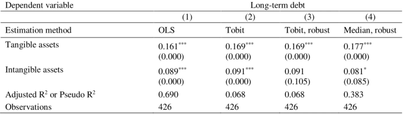
Models 1 to 3 in Panel A show that a one dollar increase in intangible assets increases leverage by $0.09 while a one dollar increase in tangible assets increases leverage by $0.17. The magnitudes are similar in the median regression in model 4 that reduces the effects of outliers. In Panel B with winsorizing, the point estimates on Tangible assets are higher than without winsorizing. The point estimates on Intangible assets decline slightly, but their significance increases in columns 3 and 4. Overall, Table 9 shows that both tangible and intangible assets support debt. On average, on a per dollar basis, intangible assets support approximately half as much debt as tangible assets.
VI. Conclusion
We show that intangible assets have a robust positive relation with leverage even though these intangible assets are not reported in firms’ financial statements and regulatory filings. On average, one dollar of intangible assets supports approximately half as much debt as one dollar of tangible assets. Intangible assets have the strongest effect on leverage in technology firms and in
18
firms with low tangible asset intensities. Our paper’s main innovation is that it circumvents the near impossibility of estimating the market value of a firm’s intangible assets by using a novel dataset that became available after a recent accounting rule change. While the dataset can only provide market value-based estimates of intangible assets for a small subset of firms, it is the first such dataset that allows a direct examination of the relation between intangible assets and financial leverage. Our results are important for the empirical research on the capital structure because they are applicable to other samples and they show that intangible assets are a primary determinant of capital structure.
19
REFERENCES
Ahern, K., Harford, J., 2013. The importance of industry links in merger waves. Journal of Finance, forthcoming.
Baker, M., Wurgler, J., 2002. Market timing and capital structure. Journal of Finance 57, 1-32. Barclay, M., Smith, C., 1995. The maturity structure of corporate debt. Journal of Finance 50,
609-631.
Campello, M., Giambona, E., 2013. Real assets and capital structure. Journal of Financial and Quantitative Analysis 48, 1-37.
Chen, L., Zhao, X., 2006. On the relation between the market-to-book ratio, growth opportunities, and leverage ratio. Finance Research Letters 3, 253-266.
Ellis, I., Jarboe, K., 2010. Intangible assets in capital markets. Intellectual Asset Management (May/June), 56-62.
Faulkender, M., Petersen, M., 2006. Does the source of capital affect capital structure? Review of Financial Studies 19, 45-79.
Flannery, M., Rangan, K., 2006. Partial adjustment toward target capital structures. Journal of Financial Economics 79, 496-506.
Frank, M., Goyal, V., 2003. Testing the pecking order theory of capital structure. Journal of Financial Economics 67, 217-248.
Frank, M., Goyal, V., 2008. Trade-off and pecking order theories of debt. In: Eckbo, B. (editor). Handbook of corporate finance: Empirical corporate finance volume 2. Elsevier/North-Holland.
Graham, J., 2000. How big are the tax benefits of debt? Journal of Finance 55, 1901-1941.
Guo, S., Fraser, M., 2010. Propensity score analysis: Statistical methods and applications. Sage Publications, Thousand Oaks.
Harford, J, 2005. What drives merger waves? Journal of Financial Economics 77, 529-560. Harris, M., Raviv, A., 1991. The theory of capital structure. Journal of Finance, 56, 297-355. Heckman, J., 1979. Sample selection as a specification error. Econometrica 47, 153-161.
Hovakimiam, A., Hovakimian, G., Tehranian, H., 2004. Determinants of target capital structure: The case of dual debt and equity issues. Journal of Financial Economics 71, 517-540.
Kale, J., Shahrur, H., 2007. Corporate capital structure and the characteristics of suppliers and customers. Journal of Financial Economics 83, 321-365.
20
Kim, W., Sorensen, E., 1986. Evidence on the impact of the agency costs of debt polic. Journal of Financial and Quantitative Analysis 21, 131-144.
Kimbrough, M., 2007. The influences of financial statement recognition and analyst coverage on the market's valuation of R&D capital. Accounting Review 82, 1195-1225.
Korajczyk, R., Levy, A., 2003. Capital structure choice: Macroeconomic conditions and financial constraints. Journal of Financial Economics 68, 75-109.
Krugman, P., 2000. Unsound bytes? New York Times, October 22, 2000.
Larkin, T., 2013. Brand perception, cash flow stability, and financial policy. Journal of Financial Economics, forthcoming.
Lemmon, M., Roberts, M., Zender, J., 2008. Back to the beginning: Persistence and the cross-section of corporate capital structure. Journal of Finance 63, 1575-1608.
Li, K., Prabhala, N., 2007. Self-selection models in corporate finance. In: Eckbo, B. (editor). Handbook of corporate finance: Empirical corporate finance volume I. Elsevier/North-Holland, 37-86.
Loumioti, M., 2012. The use of intangible assets as loan collateral. Working paper, University of Southern California.
Maksimovic, V., Phillips, G., 2001. The market for corporate assets: Who engages in mergers and asset sales and are there efficiency gains? Journal of Finance 56, 2019-2065.
Maksimovic, V., Titman, S., 1991. Financial policy and reputation for product quality. Review of Financial Studies 4, 175-200.
Mehran, H., 1992. Executive incentive plans, corporate control, and capital structure. Journal of Financial and Quantitative Analysis, 27, 539-560.
Mitchell, M., Mulherin, J., 1996. The impact of industry shocks on takeover and restructuring activity. Journal of Financial Economics 41, 193-229.
Morellec, E., 2001. Asset liquidity, capital structure and secured debt. Journal of Financial Economics 61, 173-206.
Nakamura, L. 2001. Investing in intangibles: Is a trillion dollars missing from GDP? Business Review, Federal Reserve Bank of Philadelphia, 27-37.
Nakamura, L. 2003. A trillion dollars a year in intangible investment and the new economy. In: Hand, J., Lev, B. (editors). Intangible assets. Oxford University Press.
Parsons, C., Titman, S., 2009. Empirical capital structure: A review. Foundations and Trends in Finance 3, 1-93.
21
Phillips, G., Zhdanov, A., 2013. R&D and the incentives from merger and acquisition activity. Review of Financial Studies 26, 34-78.
Rampini, A. Viswanathan, S., 2013. Collateral and capital Structure. Journal of Financial Economics 109, 466-492.
Rajan, R., Zingales, L., 1995. What do we know about capital structure? Some evidence from international data. Journal of Finance 50, 1421-1460.
Rhodes-Kropf, M., Robinson, D., Viswanathan, S., 2005. Valuation waves and merger activity: The empirical evidence. Journal of Financial Economics 77, 561-603.
Shleifer, A., Vishny, R., 1992. Liquidation values and debt capacity: A market equilibrium approach. Journal of Finance 47, 1343-1366.
Strebulaev, I., Yang, B., 2013. The mystery of zero-leverage firms. Journal of Financial Economics 109, 1-23.
Titman, S., 1984. The effect of capital structure on a firm’s liquidation decision. Journal of Financial Economics 13, 137–151.
22 Table 1: Descriptive statistics
This table reports descriptive statistics for our sample of 429 non-financial U.S. public firms that were acquired by a U.S. public acquirer between 2002 and 2011 and compares them to the Compustat universe of 82,790 non-financial firm-year observations between 2002 and 2011. Appendix B defines all variables. All variables are winsorized at the 1 and 99 percentiles. ***, **, and * denote significance at the 1%, 5% and 10% levels for the differences in means between our sample and the Compustat universe.
Compustat Our sample
mean mean sd p25 p50 p75
Assets (billion $) 3.182 1.420 *** 4.907 0.064 0.227 0.787
Long-term debt (billion $) 0.700 0.352 *** 1.258 0.000 0.003 0.170
Book leverage 0.198 0.157 *** 0.218 0.000 0.038 0.253
Market leverage 0.104 0.107 * 0.182 0.000 0.040 0.187
Market capitalization (billion $) 2.527 1.443 *** 5.086 0.064 0.268 0.889
Market-to-book 2.359 2.585 * 2.573 1.217 2.078 3.287
Sales (billion $) 2.109 1.058 *** 3.434 0.046 0.169 0.657
Operating profitability -1.503 -0.310 *** 3.323 -0.045 0.088 0.178
Cash liquidity 0.217 0.294 *** 0.254 0.058 0.229 0.501
Cash (billion $) 0.977 0.555 *** 2.039 0.023 0.104 0.331
Marginal tax rate 0.238 0.188 *** 0.152 0.020 0.210 0.341
Cash flow volatility 0.344 0.087 *** 0.151 0.020 0.047 0.100
PPE/ assets 0.268 0.194 *** 0.216 0.050 0.105 0.254 PPE (billion $) 0.983 0.447 *** 1.746 0.004 0.019 0.145 R&D/ sales 0.365 0.413 1.289 0.000 0.075 0.225 R&D (billion $) 0.028 0.030 0.082 0.000 0.006 0.025 Advertising/ sales 0.012 0.012 0.028 0.000 0.000 0.012 Advertising (billion $) 0.012 0.012 0.053 0.000 0.000 0.002 Technology industry 0.295 0.394 *** 0.489 0.000 0.000 1.000 Profit margin -1.893 -0.345 *** 1.385 -0.174 0.011 0.068 Sales growth 0.103 0.077 0.320 -0.059 0.066 0.200 Observations 82,790 429
23 Table 2: Purchase price allocation details
This table reports descriptive statistics of the purchase price allocation data, Panel A in billions of dollars and Panel B as percentages of the total purchase price allocation. Appendix B defines all variables. Panel A: In billions of dollars
mean sd p25 p50 p75 p90
Purchase price allocation 2.720 6.806 0.162 0.573 2.097 6.276
Tangible assets 1.179 3.945 0.045 0.161 0.589 2.359 Intangible assets 0.639 1.652 0.021 0.098 0.414 1.500 Technology-related 0.141 0.368 0.000 0.009 0.074 0.357 Marketing-related 0.239 0.567 0.004 0.026 0.168 0.688 Other 0.115 0.573 0.000 0.000 0.005 0.090 Goodwill 0.902 1.955 0.044 0.217 0.836 2.148
Panel B: As percentages of Purchase price allocation
mean sd p25 p50 p75 p90
Tangible assets/ PPA 36.81 23.20 19.02 32.17 50.00 72.97
Intangible asset/ PPA 24.70 17.39 11.50 22.42 34.25 48.41
TRI/ PPA 10.58 15.83 0.00 4.33 14.51 30.42
MRI/ PPA 11.13 11.24 2.63 8.45 15.73 27.40
OII/ PPA 2.96 8.99 0.00 0.00 1.24 8.25
24 Table 3: Sample distribution by industry
Panel A shows the distribution of our sample firms across the 12 Fama-Frech industries and compares it to the Compustat universe. Panel B shows the distribution of the purchase price allocation components and the proportion of firms with high tangible asset intensity across the 12 Fama-French industries. Appendix B defines all variables.
Panel A: Distribution of firms across 12 Fama-French industries
All Non-PPA sample PPA sample
N % N % N % Total 82,790 100 82,361 100 429 100 Consumer non-durables 4,564 5.5 4,547 5.5 17 4.0 Consumer durables 2,273 2.8 2,266 2.8 7 1.6 Manufacturing 8,638 10.4 8,611 10.5 27 6.3 Energy 4,460 5.4 4,445 5.4 15 3.5
Chemicals and allied products 2,381 2.9 2,373 2.9 8 1.9
Business equipment 19,035 23.0 18,859 23.0 176 41.0 Telecommunications 3,951 4.8 3,930 4.8 21 4.9 Utilities 3,669 4.4 3,663 4.5 6 1.4 Shops 8,244 10.0 8,215 10.0 29 6.8 Healthcare 11,093 13.4 11,026 13.4 67 15.6 Other (non-financial) 14,482 17.5 14,426 17.5 56 13.1
25 Panel B: Purchase price allocation components by 12 Fama-French industries
(As percentage of Purchase price allocation) Tangible assets Intangible assets Goodwill Technology-related Marketing-related Other Proportion of firms with high tangible asset intensity All industries 36.8 24.7 38.5 10.6 11.1 3.0 0.20 Consumer non-durables 30.5 36.1 33.4 0.0 30.8 5.3 0.06 Consumer durables 49.4 18.4 32.2 5.2 12.4 0.8 0.43 Manufacturing 45.1 18.4 36.5 3.1 14.1 1.2 0.33 Energy 66.7 13.2 20.1 0.4 2.1 10.7 0.38
Chemicals and allied products 56.8 17.1 26.0 4.9 10.0 2.3 0.38
Business equipment 32.1 24.0 44.0 11.8 10.6 1.6 0.13 Telecommunications 41.0 26.3 32.7 0.0 12.8 13.5 0.33 Utilities 79.6 1.0 19.4 0.0 1.0 0.0 1.00 Shops 39.7 19.1 41.3 2.0 14.3 2.6 0.43 Healthcare 24.6 39.4 36.1 30.7 5.7 2.9 0.03 Other 44.3 18.7 37.0 3.4 13.1 2.3 0.36
26 Table 4: Leverage regressions
This table shows Tobit regressions that examine the relation between intangible assets and leverage. The dependent variable in models 1 to 3 is the Book leverage and it is Market leverage in models 4 to 6. Appendix B defines all variables. p-values are in parentheses. All regressions have intercepts and use Eicker-Huber-White-Sandwich heteroskedasticity-robust standard errors clustered by industry. ***, **, and * denote significance at 1%, 5% and 10% levels, respectively.
Dependent variable Book leverage Market leverage
(1) (2) (3) (4) (5) (6)
Purchase price allocation:
Tangible assets/ PPA 0.151*** 0.146*** 0.141*** 0.139***
(0.000) (0.000) (0.000) (0.000)
Intangible assets/ PPA 0.200*** 0.250*** 0.262*** 0.074* 0.114** 0.096**
(0.004) (0.000) (0.002) (0.070) (0.013) (0.039) PPE/ assets 0.374*** 0.254*** (0.000) (0.000) Control variables R&D/ sales 0.048*** 0.039*** (0.000) (0.000) Advertising/ sales 0.588 0.348 (0.192) (0.178)
Log Market capitalization 0.000 0.003 -0.012 -0.020 -0.018 -0.030**
(0.986) (0.876) (0.463) (0.190) (0.247) (0.046) Market-to-book 0.009* 0.008* 0.007** 0.004 0.003 0.002 (0.050) (0.052) (0.050) (0.199) (0.180) (0.353) Sales 0.045** 0.041** 0.051*** 0.049*** 0.045*** 0.054*** (0.029) (0.032) (0.001) (0.004) (0.005) 0.000 Operating profitability -0.003 -0.031*** -0.031*** -0.003 -0.025*** -0.027*** (0.782) (0.000) (0.000) (0.722) 0.000 0.000 Cash liquidity -0.573*** -0.538*** -0.379*** -0.359*** -0.335*** -0.223*** (0.000) (0.000) (0.000) (0.000) (0.000) (0.001)
Marginal tax rate -0.200** -0.193** -0.181** -0.102 -0.097 -0.083
(0.026) (0.029) (0.030) (0.128) (0.143) (0.180)
Cash flow volatility -0.131 -0.101 -0.093 -0.102 -0.082 -0.089
(0.617) (0.670) (0.650) (0.542) (0.578) (0.474)
Pseudo R2 0.45 0.42 0.51 1.86 1.72 2.02
27 Table 5: Control for sample selection bias
This table reports Heckman-style estimations. The dependent variable in the first stage is the probability of being in our sample. The first stage estimations in columns 1 and 3 use the Compustat universe of 82,790 U.S. non-financial firm-year observations between 2003 and 2011. The dependent variables in the second stage are Book leverage in columns 2 and 5 and Market leverage in columns 3 and 6. The second stage uses our sample of 429 (396 after accounting for missing observations) target firms. Appendix B defines all variables. p-values are in parentheses. The regressions have intercepts and use Eicker-Huber-White-Sandwich heteroskedasticity-robust standard errors clustered by industry. ***, **, and * denote significance at 1%, 5% and 10% levels, respectively.
Dependent variable Probability in sample Book leverage Market leverage Probability in sample Book leverage Market leverage
Stage 1st stage 2nd stage 1st stage 2nd stage
(1) (2) (3) (4) (5) (6)
Tangible assets/ PPA 0.138*** 0.134*** 0.135** 0.130***
(0.006) (0.000) (0.007) (0.000)
Intangible assets/ PPA 0.152** 0.052* 0.200*** 0.080**
(0.020) (0.096) (0.006) (0.033)
R&D/ sales 0.079*** 0.035** 0.024*
(0.000) (0.021) (0.086)
Advertising/ sales 0.552 0.408 0.223
(0.360) (0.268) (0.179)
Log Market capitalization 0.004 -0.012* 0.006 -0.011*
(0.668) (0.062) (0.538) (0.072) Market-to-Book 0.014** 0.003 0.001 0.016*** 0.002 0.001 (0.020) (0.528) (0.791) (0.010) (0.681) (0.714) Sales 0.027** 0.032*** 0.026** 0.029*** (0.026) (0.000) (0.038) (0.000) Operating profitability 0.010 0.004 -0.012 -0.010* (0.416) (0.633) (0.221) (0.084) Cash liquidity -0.319*** -0.194*** -0.300*** -0.182*** (0.000) (0.000) 0.000 (0.000)
Marginal tax rate -0.129* -0.057 -0.131* -0.058
(0.075) (0.230) (0.073) (0.181)
Cash flow volatility -0.105 -0.068** -0.080 -0.057
(0.320) (0.031) (0.444) (0.359) Assets -0.013*** -0.014*** (0.000) (0.000) Profit Margin 0.046*** 0.021** (0.001) (0.011) Sales growth -0.095*** -0.051 (0.010) (0.152) Lambda -0.048 -0.061 (0.782) (0.733)
Correlation among errors -0.163** -0.182**
(0.042) (0.012)
28 Table 6: Purchase price allocation components
This table reports Tobit estimations. The dependent variable is Book Leverage in columns 1 to 3 and Market leverage in columns 4 to 6. Appendix B defines all variables. p-values are reported in parentheses. The regressions have intercepts and use Eicker-Huber-White-Sandwich heteroskedasticity-robust standard errors clustered by industry. ***, **, and * denote significance at 1%, 5% and 10% levels, respectively.
Dependent variable Book leverage Market leverage
(1) (2) (3) (4) (5) (6)
Purchase price allocation
Tangible assets/ PPA 0.144*** 0.135*** 0.130*** 0.123***
(0.001) (0.003) (0.000) (0.001) TRI/ PPA 0.096 0.178** 0.203*** 0.003 0.068*** 0.067* (0.168) (0.022) (0.004) (0.477) (0.000) (0.055) MRI/ PPA 0.186 0.200 0.290* 0.018 0.027 0.052 (0.160) (0.130) (0.058) (0.441) (0.405) (0.313) OII/ PPA 0.411*** 0.456*** 0.335* 0.278*** 0.312*** 0.217 (0.008) (0.010) (0.099) (0.005) (0.008) (0.103) PPE/ assets 0.370*** 0.238*** (0.001) (0.000) Control variables R&D/ sales 0.051*** 0.040*** (0.003) (0.000) Advertising/ sales 0.530 0.338 (0.290) (0.295)
Log Market capitalization 0.001 0.002 -0.011 -0.021 -0.020 -0.030*
(0.964) (0.915) (0.548) (0.186) (0.236) (0.055) Market-to-book 0.009** 0.008* 0.007* 0.004 0.004 0.002 (0.049) (0.053) (0.064) (0.201) (0.186) (0.362) Sales 0.043* 0.041* 0.049*** 0.048*** 0.046*** 0.054*** (0.050) (0.063) (0.005) (0.004) (0.007) (0.000) Operating profitability -0.005 -0.033*** -0.033*** -0.004 -0.027*** -0.028*** (0.646) (0.000) (0.000) (0.530) (0.000) (0.000) Cash liquidity -0.549*** -0.520*** -0.369*** -0.341*** -0.321*** -0.221*** (0.000) (0.000) (0.000) (0.000) (0.000) (0.000)
Marginal tax rate -0.211** -0.197** -0.190** -0.105 -0.094 -0.083
(0.024) (0.037) (0.031) (0.118) (0.165) (0.184)
Cash flow volatility -0.131 -0.104 -0.096 -0.104 -0.086 -0.091
(0.623) (0.657) (0.646) (0.532) (0.547) (0.458)
McFadden Adjusted R2 0.459 0.426 0.511 1.936 1.792 2.041
Cox-Snell R2 0.298 0.278 0.324 0.355 0.329 0.366
McKelvey & Zavoina R2 0.329 0.306 0.348 0.387 0.357 0.390
Observations 397 398 398 397 398 398
29 Table 7: Effect of technology industry
Panel A reports the distribution of the purchase price allocation components after splitting the sample into technology and non-technology industry firms. The last row indicates the significance of the differences between technology and non-technology industry firms. Panel B shows Tobit estimations. Book leverage is the dependent variable. All estimations contain intercepts and the same control variables as in Table 4. p-values, based on Eicker-Huber-White-Sandwich heteroskedasticity-robust standard errors clustered by industry, are in parentheses. Appendix B defines all variables. ***, **, and * denote significance at 1%, 5% and 10% levels, respectively.
Panel A: Purchase price allocation components by technology industry classification Tangible assets/ PPA Intangible assets/ PPA Goodwill/ PPA TRI/ PPA MRI/ PPA OII/ PPA Technology industry [N=169] 31.6 30.2 38.3 20.1 8.1 2.0 Non-technology industry [N=260] 40.2 21.1 38.6 4.4 13.1 3.6 Significance of difference *** *** *** *** *
30
Panel B: Tobit models with Technology industry interactions
Dependent variable Book leverage
Model (1) (2) (3) (4) (5)
Tangible assets/ PPA 0.109* 0.114* 0.095** 0.089**
(0.092) (0.093) (0.021) (0.033)
Tangible assets/ PPA * Technology industry 0.027 -0.026
(0.856) (0.867)
Intangible assets/ PPA 0.138 0.170*
(0.129) (0.052)
Intangible assets/ PPA * Technology industry 0.227* 0.257*
(0.061) (0.031)
TRI/ PPA -0.387* -0.298
(0.070) (0.237)
TRI/ PPA* Technology industry 0.699*** 0.697***
(0.001) (0.006)
MRI/ PPA 0.215 0.217
(0.308) (0.270)
MRI/ PPA * Technology industry -0.186 -0.197
(0.310) (0.311)
OII/ PPA 0.280** 0.290**
(0.037) (0.031)
OII/PPA * Technology industry 0.442 0.572
(0.255) (0.151) Technology industry -0.070*** -0.140** -0.131* -0.113*** -0.121*** (0.009) (0.046) (0.071) (0.000) (0.000) R&D/ sales 0.056*** 0.045*** 0.046*** (0.000) (0.000) (0.000) Advertising/ sales 0.300 0.324 0.218 (0.565) (0.490) (0.681)
Other Firm Characteristics as in Table 4 Yes Yes Yes Yes Yes
Pseudo R2 0.449 0.473 0.445 0.502 0.471
31
Table 8: Leverage regressions by tangible asset intensity
This table shows Tobit estimations separately for firms with low and high tangible asset intensities. We classify tangible asset intensity as high if the tangible assets comprise more than 66% of the total purchase price allocation. The dependent variable is Book leverage in columns 1 to 4 and Market leverage in columns 5 to 8. Appendix B defines all variables. All estimations include intercepts. p-values, based on Eicker-Huber-White-Sandwich heteroskedasticity-robust standard errors clustered by industry, are in parentheses. ***, **, and * denote significance at 1%, 5% and 10% levels, respectively.
32 Tangible assets/ PPA Bottom 2
terciles Top tercile Bottom 2 terciles Top tercile Bottom 2 terciles Top tercile Bottom 2 terciles Top tercile
Tangible asset intensity low high low high low high low high
Dependent variable Book leverage Market leverage
(1) (2) (3) (4) (5) (6) (7) (8)
Purchase price allocation
PPE/ assets 0.400* 0.350*** 0.406* 0.381*** 0.187** 0.252*** 0.191** 0.278***
(0.054) (0.000) (0.053) (0.000) (0.037) (0.000) (0.034) (0.000)
Intangible assets/ PPA 0.302*** -0.061 0.306*** -0.095 0.153*** -0.049 0.157*** -0.079
(0.002) (0.811) (0.002) (0.670) (0.001) (0.839) (0.001) (0.720) Control variables R&D/ sales 0.014 0.104*** 0.013* 0.090*** (0.000) (0.000) (0.098) (0.000) Advertising/ sales 0.505 0.518 0.266 0.508 (0.426) (0.310) (0.384) (0.282)
Log Market capitalization -0.015 -0.006 -0.012 -0.018 -0.034** -0.017 -0.031** -0.028
(0.432) (0.789) (0.538) (0.521) (0.012) (0.409) (0.028) (0.276) Market-to-book 0.005 0.022 0.005 0.022* 0.002 0.008 0.002 0.008 (0.361) (0.117) (0.415) (0.097) (0.341) (0.376) (0.399) (0.305) Sales 0.052** 0.043** 0.049** 0.053* 0.055*** 0.047** 0.052*** 0.056** (0.019) (0.045) (0.032) (0.071) (0.000) (0.033) (0.001) (0.043) Operating profitability -0.021 -0.039*** -0.030*** -0.041*** -0.015* -0.035*** -0.023*** -0.035*** (0.111) (0.009) (0.000) (0.007) (0.082) (0.002) 0.000 (0.001) Cash liquidity -0.475*** -0.341*** -0.454*** -0.176 -0.265*** -0.291*** -0.252*** -0.147 (0.000) (0.000) (0.000) (0.308) (0.000) (0.000) (0.000) (0.338)
Marginal tax rate -0.216 -0.208 -0.197 -0.136 -0.097 -0.134 -0.086 -0.073
(0.104) (0.205) (0.117) (0.427) (0.243) (0.388) (0.291) (0.649)
Cash flow volatility -0.171 -0.504** -0.112 -0.275 -0.134 -0.405** -0.095 -0.190
(0.511) (0.042) (0.625) (0.416) (0.380) (0.048) (0.480) (0.473)
Pseudo R2 0.48 0.84 0.47 0.65 2.06 1.17 2.03 0.87
33
Table 9: Quantifying debt supported by tangible and intangible assets
This table reports a series of OLS, Tobit, and median regression models. The dependent variable is Long-term debt. The only independent variables are Tangible asset and Intangible Assets. We do not include additional explanatory variables because of the substantial correlations of the variables measured in dollar amounts. Appendix B defines all variables. p-values are in parentheses. The regressions have intercepts and use different methods to estimate the significance of the standard errors, namely simple and robust standard errors, as reported in each column. ***, **, and * denote significance at 1%, 5% and 10% levels, respectively.
Panel A: Unwinsorized
Dependent variable Long-term debt
(1) (2) (3) (4)
Estimation method OLS Tobit Tobit, robust Median, robust
Tangible assets 0.161*** 0.169*** 0.169*** 0.177*** (0.000) (0.000) (0.000) (0.000) Intangible assets 0.089*** 0.091*** 0.091 0.081* (0.000) (0.000) (0.105) (0.085) Adjusted R2 or Pseudo R2 0.690 0.068 0.068 0.383 Observations 426 426 426 426
Panel B: Winsorized at 5% and 95%
Dependent variable Long-term debt
(1) (2) (3) (4)
Estimation method OLS Tobit Tobit, robust Median, robust
Tangible assets 0.251*** 0.278*** 0.278*** 0.317*** (0.000) (0.000) (0.000) (0.000) Intangible assets 0.072*** 0.081*** 0.081** 0.047** (0.000) (0.001) (0.037) (0.030) Adjusted R2 or Pseudo R2 0.644 0.073 0.073 0.404 Observations 426 426 426 426
34 Appendix A
Appendix A.1: Acquirer: ZHONE TECHNOLOGIES INC. Target: Sorrento Networks Corporation
FORM 10-K FOR THE PERIOD ENDED DECEMBER 31, 2004. ZHONE TECHNOLOGIES INC (Filer) CIK: 0001101680
http://www.sec.gov/Archives/edgar/data/1101680/000119312505052811/d10k.htm pg. 57
Purchased Technology
The Company recorded purchased technology related to acquisitions of $9.2 million, and $2.2 million during the years ended December 31, 2004, and 2003, respectively. To determine the values of purchased technology, the expected future cash flows of the existing developed technologies were discounted taking into account the characteristics and applications of the product, the size of existing markets, growth rates of existing and future markets, as well as an evaluation of past and anticipated product lifecycles.
(a) Sorrento Networks Corporation
In July 2004, the Company completed the acquisition of Sorrento Networks Corporation in exchange for total consideration of $98.0 million, consisting of common stock valued at $57.7 million, options and warrants to purchase common stock valued at $12.3 million, assumed liabilities of $27.0 million, and acquisition costs of $1.0 million. The Company acquired Sorrento to obtain its line of optical transport products and enhance its competitive position with cable operators. One of the Company’s directors is a partner of a venture capital firm which is a significant stockholder of Zhone, and which also held warrants to purchase Sorrento common stock that were assumed by Zhone.
The purchase consideration was allocated to the fair values of the assets acquired as follows: net tangible assets—$23.4 million, amortizable intangible assets—$14.8 million, purchased in-process research and development—$2.4 million, goodwill—$57.2 million and deferred
compensation—$0.2 million. The amount allocated to purchased in-process research and development was charged to expense during the third quarter of 2004, because technological feasibility had not been established and no future alternative uses for the technology existed. The estimated fair value of the purchased in-process research and development was determined using a discounted cash flow model, based on a discount rate which took into consideration the stage of completion and risks associated with developing the technology. Of the amount allocated to amortizable intangible assets, $9.2 million was allocated to core technology, which is being amortized over an estimated useful life of five years. The remaining $5.6 million was allocated to customer relationships, which is being amortized over an estimated useful life of four years.