Department of Econometrics and Business Statistics
http://www.buseco.monash.edu.au/depts/ebs/pubs/wpapers/Two canonical VARMA forms:
Scalar component models
vis-à-vis the Echelon form
George Athanasopoulos, D. S. Poskitt and
Farshid Vahid
First draft July 2007
Revised May 2009
component models vis-à-vis the
Echelon form
George Athanasopoulos
Department of Econometrics and Business Statistics, Monash University, VIC 3800, Australia.
Email: [email protected]
D. S. Poskitt
Department of Econometrics and Business Statistics, Monash University, VIC 3800, Australia.
Email: [email protected]
Farshid Vahid School of Economics,
Australian National University, ACT 0200, Australia. Email: [email protected]
18 May 2009
component models vis-à-vis the
Echelon form
Abstract: In this paper we study two methodologies which identify and specify canonical form VARMA models. The two methodologies are: (i) an extension of the scalar component methodology which specifies canonical VARMA models by identifying scalar components through canonical cor-relations analysis; and (ii) the Echelon form methodology, which specifies canonical VARMA models through the estimation of Kronecker indices. We compare the actual forms and the methodologies on three levels. Firstly, we present a theoretical comparison. Secondly, we present a Monte-Carlo simulation study that compares the performances of the two methodologies in identifying some pre-specified data generating processes. Lastly, we compare the out-of-sample forecast performance of the two forms when models are fitted to real macroeconomic data.
Keywords: Echelon form, Identification, Multivariate time series, Scalar components, VARMA model.
1 Introduction
Macroeconomists analyse and forecast aggregate economic activity by studying the dynamics of eco-nomic variables such as GDP growth, unemployment and inflation. Univariate autoregressive inte-grated moving average (ARIMA) processes are a useful class of models for capturing and describing the dynamics of such series. Box and Jenkins (1970) popularised this useful univariate methodol-ogy, making it arguably the most well known time series tool. However, ARIMA modelling is limited by its inability to capture and model important dynamic inter-relationships between variables of in-terest. The direct generalisation of the stationary ARMA model to the multivariate form leads to the vector ARMA or VARMA model (see amongst others, Quenouille, 1957; Tunnicliffe-Wilson, 1973;
Tiao and Box,1981; Tsay, 1989;Tiao, 2001). This generalisation has been proven to be far from trivial. One of the major issues faced by researchers in the multivariate time series field of VARMA modelling relates to the identification of unique representations. The issues of identification have been discussed over the years by many researchers, includingHannan(1969,1970,1976),Hannan and Deistler(1988),Lütkepohl(1993) andReinsel(1997). In this paper we study and compare two methodologies that overcome this issue and achieve unique canonical VARMA representations.
“While VARMA models involve additional estimation and identification issues, these compli-cations do not justify systematically ignoring these moving average components, as in the SVAR approach.”
Cooley and Dwyer(1998)
The complexities of identifying and estimating unique VARMA models, and, in sharp contrast, the ease of specifying and estimating vector autoregressions (VARs) have resulted in VARs, dominating the macroeconomic literature, despite ubiquitous warnings about their many practical and theoreti-cal shortcomings. For example, in contrast to VARMA models, VARs are not invariant to aggregation, marginalisation or measurement error. Hence, to avoid misspecification, any modelling of macroe-conomic aggregates (such as gross domestic product, industrial production, etc.) should include moving average dynamics, even if the components of these aggregates are assumed to follow finite autoregressive processes. Furthermore, even if we assume a finite order VAR representation for a set of macroeconomic aggregates, modelling a subset of these should again include moving average dy-namics (see for exampleZellner and Palm,1974;Fry and Pagan,2005).Ravenna(2007) warns that caution should be used by researchers using finite order VARs to build dynamic stochastic general equilibrium (DSGE) models, andFernández-Villaverde et al.(2005) show that linearised versions of DSGE models generally imply a finite order VARMA structure.
The first methodology we consider that returns unique VARMA representations is the Athanasopou-los and Vahid(2008a) extension ofTiao and Tsay(1989). This methodology comprises three stages. In the first stage, “scalar component models” (SCMs) embedded in the VARMA model are identified using a series of tests based on canonical correlations analysis between judiciously chosen sets of variables. In the second stage, a fully identified structural form is developed through a series of
logical deductions and additional canonical correlations tests. Then, in the final stage, the identified model is estimated using full information maximum likelihood (FIML) (Durbin,1963). We present the scalar component methodology in Section2.
The second methodology we consider is the Echelon form methodology, which involves specifying canonical Echelon form models through the estimation of Kronecker indices. Kronecker indices are simply the maximal row degrees of each individual equation of a VARMA model, and are estimated through a series of least squares regressions. This methodology has been developed by many time series analysts such as Akaike (1974, 1976),Kailath (1980), Hannan and Kavalieris(1984), Solo
(1986), Hannan and Deistler (1988), Poskitt (1992) and Lütkepohl and Poskitt (1996), among others. We present the Echelon form methodology in Section3.
“We see that dealing with VARMA models in Echelon form is not as easy as dealing with uni-variate ARMA models .... This might be a reason why practitioners are reluctant to employ VARMA models. Who could blame them for sticking with VAR models when they probably need to refer to a textbook to simply write down an identified VARMA representation?”
Dufour and Pelletier(2008)
Specifying a unique Echelon form VARMA representation involves applying a set of mathematical rules. The advocates of the Echelon form portray this as its major advantage. However, the com-plexities of the formulae and the apparent lack of intuition behind these formulae have earned this methodology the reputation of being a very complicated method, and have not helped to promote the application of VARMA models in the empirical literature. In Section4we theoretically connect the Echelon form to SCMs. This connection provides an intuition behind the complicated Echelon form formulae and shows that understanding theAthanasopoulos and Vahid(2008a) scalar method-ology demystifies the Echelon form and eliminates the need for a textbook.
Although many studies have contributed to the Echelon form methodology, no investigation has been undertaken into the finite sample performance of this methodology when attempting to iden-tify VARMA models. In Section4.1we conduct Monte-Carlo experiments, and evaluate the ability of both the Echelon form and the SCM methodology to identify some pre-specified VARMA data generating processes (DGPs).
Using real data, Athanasopoulos and Vahid(2008b) conclude that VARMA models specified by the scalar component methodology forecast macroeconomic variables more accurately than VARs. In Section 5 we compile 70 trivariate data sets and perform a similar forecasting exercise. We eval-uate the forecasting performance of VARMA models specified by the SCMs versus VARMA models specified by the Echelon form methodology and VAR models with lag lengths chosen by AIC and BIC.
2 A VARMA modelling methodology based on scalar components
The scalar component methodology we employ is the Athanasopoulos and Vahid (2008a) exten-sion of the Tiao and Tsay (1989) methodology. In this section we present a brief overview of the methodology. For more details, readers should refer to the above mentioned papers.
Stage I: Identification of the scalar components
The aim of identifying scalar components is to examine whether there are any simplifying embedded structures underlying a VARMA(p,q) process. These simple structures (or scalar components) are linear combinations of variables that depend on fewer thanp autoregressive lags and fewer thanq lags of innovations. Formally, for a givenK−dimensional VARMA(p,q)process
yt=Φ1yt−1+. . .+Φpyt−p+εt−Θ1εt−1−. . .−Θqεt−q, (1)
a non-zero linear combinationzt =α0yt follows an SCM(p1,q1)ifαsatisfies the following proper-ties:
α0Φp1 6= 0where 0≤p1≤p; α0Φl = 0forl=p1+1, . . . ,p; α0Θq1 6= 0where 0≤q1≤q;
α0Θl = 0forl=q1+1, . . . ,q.
The SCM methodology uses a sequence of canonical correlations tests until it discovers K such linear combinations, starting from the most parsimonious SCM(0, 0). Denoting the squared sample canonical correlations betweenYm,t≡(y0t, . . . ,y0t−m)andYh,t−1−j≡(y0t−1−j, . . . ,yt−0 1−j−h)0byλb1< b
λ2<. . .<λKb , the test statistic suggested byTiao and Tsay(1989) for testing for the null of at least sSCM(pi,qi)against the alternative of fewer thansscalar components is
C(s) =− n−h− j s X i=1 ln ( 1−λib di ) a sχs×{2 (h−m)K+s}, (2)
where di is a correction factor that accounts for the fact that the canonical variates in this case can be moving averages of order j. Specifically,
di=1+2 j X v=1 b ρv b ri0Ym,t b ρv b gi0Yh,t−1−j , (3)
where ρbv(.) is the vth order autocorrelation of its argument and rb0iYm,t and gb
0
iYh,t−1−j are the
Suppose we have K linearly independent scalar components characterized by the transformation matrixA= α1, . . . ,αK
0
. If we rotate the system in equation (1) byA, we obtain
Ayt=Φ∗1yt−1+. . .+Φ∗pyt−p+ε∗t−Θ∗1ε∗t−1−. . .−Θ∗qε∗t−q, (4) whereΦ∗i =AΦi, ε∗t =Aεt andΘ∗i =AΘiA−1, in which the right hand side coefficient matrices may have many rows of zeros. However, if there are scalar components SCM(pr,qr)and SCM(ps,qs)
which are strongly nested, i.e. whenpr> ps andqr>qs, then even if we knowA, the system will not be identified. This is because SCM(ps,qs)implies an exact linear relationship between the lagged
variables on the right hand side of SCM(pr,qr). In such cases, min{pr−ps,qr−qs}, autoregressive or moving average parameters must be set to zero for the system to be identified. We set the moving average parameters to zero in such situations. This is often referred to as the “general rule of elimination”.
Stage II: Placing identification Restrictions on Matrix
A
Not all parameters inAare free parameters. We can multiply each row ofAby a constant without changing the structure of the system. We can also linearly combine an SCM with any other SCM with weakly smallerpandqand not change its order. These simple implications of the definition of scalar components leads to the following identification rules that, asAthanasopoulos and Vahid (2008a) show, lead to a uniquely identifiedA. We refer to this system as a canonical SCM representation. These rules are:
1. Normalize one parameter in each row ofAto one.Athanasopoulos and Vahid(2008a) suggest a procedure to safeguard against the possibility of normalising on a zero parameter; we do not repeat it here to save space.
2. In all cases where there are two embedded scalar components with weakly nested orders, i.e., p1 ≥ p2 and q1 ≥ q2, if the parameter in the ith column of the row ofA corresponding to the SCM p2,q2
is normalized to one, the parameter in the same position in the row ofA corresponding to SCM(p1,q1)should be restricted to zero.
Stage III: Estimation of the Uniquely Identified System
Estimate the parameters of the system using FIML. The canonical correlations procedure produces good starting values for the parameters, in particular for the SCMs with no moving average compo-nents. Alternatively, lagged innovations can be estimated from a long VAR and used for obtaining initial estimates for the parameters, as in Hannan and Rissanen(1982). The maximum likelihood procedure provides estimates and estimated standard errors for all parameters, including the free parameters in A. All usual considerations that ease the estimation of structural forms are also
applicable here, and should definitely be exploited in estimation.
3 Canonical Reverse Echelon Form
AK−dimensional VARMA representation, such as
Ψ(L)yt=Ξ(L)εt, (5) whereΨ(L) =Ψ0−Ψ1L−. . .−ΨpLpandΞ(L) =Ξ0−Ξ1L−. . .−ΞqLq is said to be in reverse
Echelon form (Lütkepohl and Claessen,1997) if the pair of polynomials in the lag operatorsΨ(L) = ψr c(L) r,c=1,...,K andΞ(L) = ξr c(L)
r,c=1,...,K, [Ψ(L):Ξ(L)], are left coprime and possess the
following properties:
1. Ψ0=Ξ0 is lower triangular with unit diagonal elements,
2. rowr of the polynomial operators[Ψ(L):Ξ(L)]is of maximum degreekr,
3. the operators have the form of
ξr r(L) =1− kr X j=1 ξ(j) r rL j for r=1, . . . ,K, ξr c(L) =− kr X j=kr−kr c+1 ξ(j) r c L j for r 6 =c, ψr c(L) =ψ(r c0)− kr X j=1 ψ(j) r c L j withψ(0) r c =ξ( 0) r c forr,c=1, . . . ,K,
whereψ(r cj)specifies the element ofΨj in rowr and columnc, andξ( j)
r c specifies the element
ofΞj in rowr and columnc.
The maximum row degreesk= (k1, . . . ,kK)0are called theKronecker Indicesand define the
struc-ture of the system, and
kr c= min(kr+1,kc) for r≥c min(kr,kc) for r <c ,
for r,c = 1, . . . ,K, specifies the number of free parameters in the operatorψr c(L) forr 6= c. The sum of the Kronecker indicesm=PKr=1kr is called theMcMillan degree. The maximum number of freely varying parameters isd(k) =2mK.
The theory and examples of the Echelon form representation of VARMA models are given by Solo
(1993), among others. The “reverse Echelon form” defined above is a variant of the Echelon form in which whenever identification can be achieved by placing a zero restriction on either an autore-gressive parameter or on a moving average parameter, the moving average parameter is set to zero. Note that just as in the SCM representation, a reverse Echelon form is a rotation of the VARMA model, here by the matrixΨ0 that turns cross equation restrictions into zero restrictions and makes
the system identifiable.
The complicated looking definitions of the canonical Echelon form and reverse Echelon form have baffled practitioners and led to comments such as the one quoted above fromDufour and Pelletier
(2008). However, as we show below, by understanding the relationship between Kronecker indices and orders of scalar components, one can see that the above definition is nothing but the symbolic representation of identification rules in a special sub-class of scalar component models. To under-stand that, we need to explain the relationship between Kronecker indices and Kronecker invariants. An Echelon form or a reverse Echelon form representation is not invariant with respect to an arbi-trary reordering of the Kronecker indices. A reordering of the Kronecker indices may change the structure of the left hand side matrix, which contains the contemporaneous relationships. However, the variables in yt can be permuted such that the Kronecker indices are arranged in descending
order (seePoskitt,2005).
Definition 1 When the Kronecker indices ofyt are such that k1≥k2. . .≥kK, these are referred to as
Kronecker invariants.
When a VARMA system is expressed in terms of Kronecker invariants it not only has a canonical form, but it also has a unique representation for each row of the system; i.e., even if further order preserving permutations are possible (by changing the order of two indices that are equal to each other), the structure of the system will not change.
Example 2 Consider a trivariate stable and invertible VARMA process with Kronecker invariantsk=
(k1,k2,k3)0= (1, 1, 0)0. The total number of freely varying parameters is d(k) =2mK=2×2×3=12.
The reverse Echelon form representation of the process is 1 0 0 0 1 0 ψ(0) 31 ψ (0) 32 1 yt= ψ(1) 11 ψ (1) 12 ψ (1) 13 ψ(1) 21 ψ (1) 22 ψ (1) 23 0 0 0 yt−1+Ξ0εt− ξ(1) 11 ξ (1) 12 0 ξ(1) 21 ξ (1) 22 0 0 0 0 εt−1. (6)
It is obvious from the example that if we change the order of the first two variables, Kronecker invariants will not change and the structure of the system (i.e. the position of zeros and ones in the system) remains unchanged. Poskitt’s (1992) search process is a simple and efficient procedure for the practical specification of Echelon form VARMA models, and is based on searching for Kronecker invariants. We use Poskitt’s procedure in the empirical section of this paper. A brief summary of this
procedure is as follows.
Stage I: Obtaining approximate residuals
A long order VAR(h) is fitted and the estimated residuals εbt(h) are obtained. These are used as estimates of the lagged innovations in subsequent stages. As suggested by Lütkepohl and Poskitt
(1996), we takeh=ln(T). The general idea is thathhas to be greater than the largest Kronecker index.
Stage II: Searching for Kronecker invariants
Using the estimated residuals from Stage I, Echelon form VARMA models of the form yt=Ψ1yt−1+. . .+Ψpyt−p+ Ψ0−IK
b
εt(h)−yt
+Ξ1εbt−1(h) +. . .+Ξqεbt−p(h) +εt are fitted for a range of Kronecker indices. The optimum model is selected based on model selection criteria. There are two issues that need to be addressed here. These are: (i) which efficient pro-cedure for searching for the optimal set of Kronecker indices should be used, and (ii) which model selection criterion should be used.
We employ Poskitt’s (1992) search procedure coupled with the BIC as the model selection criterion. From extensive Monte-Carlo experiments we have concluded that the BIC outperforms the AIC and the HQ, especially for sample sizes of 200 observations or more. For smaller samples the HQ may also be considered.1
Poskitt’s (1992) search procedure explores a significant property of Echelon forms. The restrictions of the rthequation imposed by a set of Kronecker indicesk= (k1, . . . ,kK)0depend on the Kronecker
indiceski≤kr. They do not depend on indices greater thankr. If we consider Kronecker invariants, this means that the structure of each equation depends on the structure of equations in the block with the same Kronecker index and other equations below that block.
Using this property, the search starts with all Kronecker invariants being set to zero. We compute the BIC for each equation of the model; i.e., we compute BICr(kr) ∀kr = 0, and compare this to BICr(kr) ∀kr = 1, for r =1, . . . ,K. For any BICr(0)≤BICr(1)we fix kr =0. All other invariants are incremented, and we fix kr = 1 for any BICr(1) ≤BICr(2). This process is repeated until all
Kronecker invariants are fixed.
1These Monte-Carlo simulation results come from the unpublished PhD dissertation ofAthanasopoulos(2007) and are available upon request.
Stage III: Estimation of the identified system
Efficient parameter estimates of the uniquely identified Echelon form VARMA model with Kronecker invariantskare obtained using FIML.
4 Scalar Components vis-à-vis Echelon Form
Tsay(1991) explored the scalar components implications of an Echelon form with a set of Kronecker indices. However, at that time it was not possible to establish a direct correspondence between the Echelon form and the existing scalar component methodologies, because the scalar component methodology ofTiao and Tsay(1989) did not specify the structure of the left hand side parameter matrixA. However, the scalar component methodology ofAthanasopoulos and Vahid(2008a) that we describe above specifies a complete structure, and in the following theorem we establish the relationship between a VARMA model identified using the order of its embedded scalar components and a VARMA model in Echelon form identified via its Kronecker invariants.
Theorem 3 Suppose thatyt is a stable and invertible VARMA process represented in reverse canonical Echelon form with Kronecker invariants k = k1, . . . ,kK
0
, where k1 ≥ . . . ≥ kK and the McMillan
degree is m =PKr=1kr <∞. Now suppose thatyt is also represented in a canonical SCM form that consists of K−SCMs of orders sr = (pr,qr) for r = 1, . . . ,K. The set of Kronecker invariants k is equivalent to a set of SCM orderssmax= (smax1 , . . . ,smaxK )0, where smaxr =max pr,qr
for r=1, . . . ,K. Furthermore, if pr = qr ∀ r = 1, . . . ,K then the reverse canonical Echelon form and the canonical SCM form are identical if the same permutation of variables with equal indices are chosen, and after innovations are rewritten in the same way.
Proof. The first part of the theorem is the same as Theorem 5 of Tsay (1991). Here we show that if pr = qr ∀ r = 1, . . . ,K then the reverse canonical Echelon form and the canonical SCM form are equivalent. Since Kronecker invariants are in descending order, the reverse Echelon form rules imply a VARMA(k1,k1) model in which the Ψk1−j and Ξk1−j matrices have rows of zeros in all rows with
Kronecker invariants kr such that k1−kr > j for j =0, . . . ,k1−1. Since Kronecker invariants are in descending order, these rows of zeros are the bottom rows of these matrices. In addition, in any row of the moving average matrices where a zero appears at position c, all elements of that row to the right of c will be zero. Finally, theΨ0andΞ0matrices are lower triangular with unit diagonals, are equal to each
other, and have identity submatrices that start from position ψ(r r0)and end at position ψ(ss0) whenever kr =kr+1 =· · ·=ks. In the SCM representation, when pr =qr ∀r =1, . . . ,K and we arrange these components in descending order, the first part of this theorem ensures that pr = kr. The definition of
scalar components of order pr=qr∀r=1, . . . ,K and the “general rule of elimination” described above imply an SCM representation with autoregressive and moving average parameter matrices with zeros in exactly the same positions as those for the reverse Echelon form described above. Also, since the SCMs
are arranged in descending order, the identification rules in Section2imply that theAmatrix is lower triangular, with identity blocks as described above whenever the SCMs are of the exact same order. This means that the matrices[Ψ0,Ψ1, . . . ,Ψp,Ξ1, . . . ,Ξq]in (5) and[A,Φ∗1, . . . ,Ψ∗p,Θ∗1, . . . ,Θ∗q]have the
exact same structure. The only difference there can be between the reverse Echelon form implied by the Kronecker invariants and the structure implied by scalar components is that the order of variables with the exact same indices can be permuted, which is inconsequential, and that the former is stated in terms of the innovations in each variable, while the latter is in terms of innovations in the scalar components. However, if we rewrite the innovations of the scalar components model in terms of the innovation in each variable using the relationship"∗t =A"t, the structure of the moving average matrices will not change because when any lower diagonal matrix is pre-multiplied by a row vector which has zeros at position c and everywhere to the right of c, the outcome will be a row vector with the exact same structure. This completes the proof.
Example 4 Consider the VARMA(1, 1)process 1 0 0 0 1 0 a31 a32 1 yt= φ∗ 11 φ12∗ φ∗13 φ∗ 21 φ22∗ φ∗23 0 0 0 yt−1+ε∗t− θ∗ 11 θ12∗ 0 θ∗ 21 θ22∗ 0 0 0 0 ε∗t−1. (7)
This process is a canonical SCM representation and consists of three SCMs of orders (1, 1), (1, 1) and (0, 0). Obviously, as Theorem (3) predicts, this model has Kronecker invariants k = smax =
(max(1, 1), max(1, 1), max(0, 0))0 = (1, 1, 0). If we substitute A"t and A"t−1 for "∗t and "∗t−1, the
structure of the moving average parameter matrix does not change, and the resulting system is the reverse Echelon form of a system with Kronecker invariants(1, 1, 0).
Having considered a situation where the canonical SCM and Echelon forms are identical, we now present an example where this is not the case.
Example 5 Consider the VARMA process consisting of three SCMs of orders(1, 1),(1, 0)and(0, 0), 1 0 0 a21 1 0 a31 a32 1 yt= φ∗ 11 φ12∗ φ∗13 φ∗ 21 φ22∗ φ∗23 0 0 0 yt−1+ε∗t− θ∗ 11 θ12∗ 0 0 0 0 0 0 0 ε∗t−1. (8)
Notice now that for the second SCM, the “autoregressive” order is different from the “moving average” order, i.e., pr 6=qr for r = 2. According to Theorem (3), the corresponding Echelon form model has
Kronecker indices
Thus, the canonical reverse Echelon form representation is 1 0 0 0 1 0 ψ(0) 31 ψ (0) 32 1 yt= ψ(1) 11 ψ (1) 12 ψ (1) 13 ψ(1) 21 ψ (1) 22 ψ (1) 23 0 0 0 yt−1+ Ψ0εt− ξ(1) 11 ξ (1) 12 0 ξ(1) 21 ξ (1) 22 0 0 0 0 εt−1, (9)
as in equation (7) withξ(211)=−a21ξ(111)andξ (1)
22 =−a21ξ(121). The Echelon form specification does not
impose this restriction, whilst the SCM methodology discovers it and transforms the system to translate this restriction into a row of zeros in the moving average parameter matrix. This leads to a system with 11 free parameters rather than 12. This shows that VARMA models with SCMs with pr 6=qr for some r are rank restricted versions of reverse Echelon forms with Kronecker indices kr =max(pr,qr)
for r=1, . . . ,K.
The above example shows that the SCM methodology discovers some additional restrictions com-pared to the Echelon form methodology. Since Hannan’s Theorem (Hannan and Deistler, 1988) proves that the restrictions in the Echelon form are necessary and sufficient restrictions for the unique identification of the VARMA models, we can conclude that the extra restrictions discovered by the SCM methodology are restrictions that are supported by the data over and above the neces-sary conditions for identification.
Theorem3shows that theAthanasopoulos and Vahid(2008a) SCM methodology complements the Echelon form methodology and helps us avoid the otherwise necessary reference to the complicated formulae involved with the specification of Echelon form VARMA models. Given a set of Kronecker invariants, applying Stage II of the scalar component methodology can identify a parameter space for a unique VARMA representation which is identical to the parameter space specified by the Echelon form formulae. However, it is important to highlight that these formulae are what makes the Echelon form very attractive and applicable when programming an identification process for VARMA models.
4.1 A Monte Carlo Evaluation
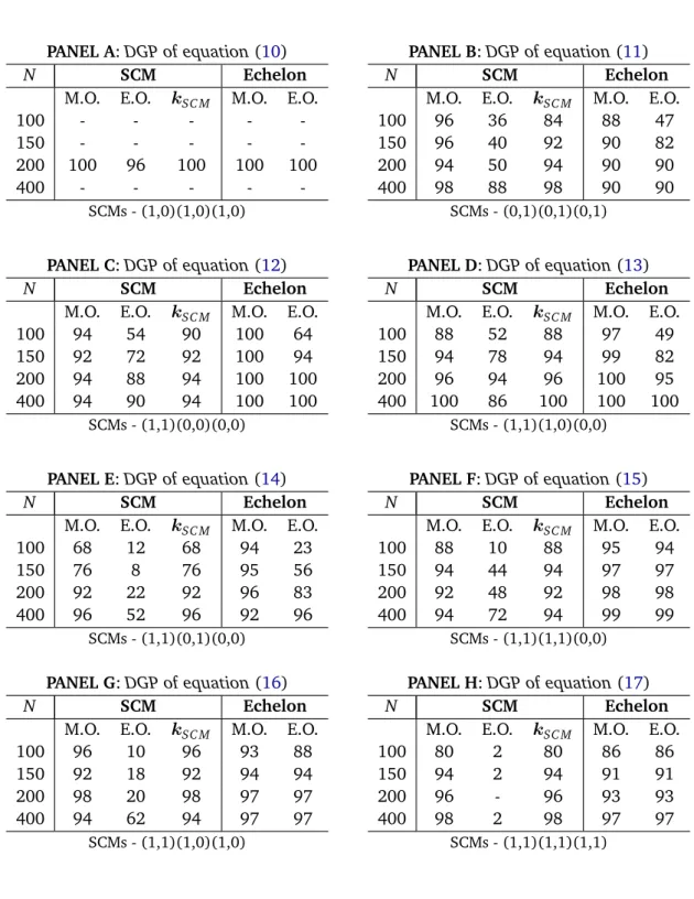
In this section we perform Monte Carlo experiments in order to evaluate the performance of the identification procedures when identifying some pre-specified VARMA data generating processes (DGPs). We consider the DGPs presented in Appendix A, for sample sizes N = 100, 150, 200 and 400 observations. Due to the long, manual and challenging process of identifying SCMs, only 50 iterations were performed for each process and for each sample size. In contrast, we managed to automate Poskitt’s search procedure for the Echelon form methodology, and therefore 1000 itera-tions were performed for each model and for each sample size. The results are presented in Table
1.2
2We should note that these results are a summary of the more elaborate tables presented for each individual DGP in the unpublished PhD dissertation ofAthanasopoulos(2007). These individual results are available upon request.
In comparing these results, extra attention is required as canonical SCMs and Echelon form models are identical only whenpr=qr∀r=1, . . . ,K as shown by Theorem3.
The first two columns under SCM in each panel in Table1show the percentage of times the SCM methodology correctly specifies the maximal order (M.O.) and the exact order (E.O.) of the DGP. The two columns in each panel under “Echelon” show these figures for the Echelon form methodology. However, maximal order and exact order are not the same concept in the two model forms. The M.O. pSC M,qSC M
in the SCM case is the maximum “autoregressive”, pSC M = max p1, . . . ,pK
, and “moving average”,qSC M =max q1, . . .qK
, order of all the scalar components identified. This corresponds to the order of the identified VARMA(pSC M,qSC M) model. In the Echelon form, the
maximum order corresponds to the maximum Kronecker index identified, i.e., max(k1, . . . ,kK). This
yields a VARMA(pEC H,qEC H), where pEC H = qEC H = max(k1, . . . ,kK). Therefore, if the DGP is a
VARMA(p,q) with p =q, the maximum orders are exactly equivalent; however, if p6= q they are not equivalent. The SCM methodology attempts to identify the p andq orders separately, but the Echelon form attempts to identify the maximum ofpandq, i.e., max(p,q).
As with the maximum order, the exact order (E.O.) results are not exactly equivalent either. The exact order being specified correctly by the SCM procedures implies that all “autoregressive” and “moving average” components of the model under consideration have been specified correctly. That is, the procedure identified exactly the SCMs specified below each section of the table. In contrast, the exact order being specified correctly by the Echelon form methodology means that the Kronecker indices, i.e., the maximum row degrees kr for r = 1, . . . ,K, of the model have been identified
correctly.
To make these results comparable, the third column of each panel under SCM, labeledkSC M, shows the percentage of times the scalar component methodology correctly identifies the Kronecker indices of the model. This is then directly comparable to the E.O. of the Echelon form. To clarify how this information is extracted from the simulation results, we present the following example.
Example 6 Consider the processes of equations (16), 1 0 0 0.4 1 0 0 −0.6 1 yt= 0.7 −0.6 0.4 0.6 −0.5 −0.4 0.3 −0.6 0.4 yt−1+εt− 0.7 0.4 −0.6 0 0 0 0 0 0 εt−1, and (15) 1 0 0 0 1 0 0.5 −0.7 1 yt= 0.7 −0.5 0.7 0.6 0.3 0.6 0 0 0 yt−1+εt− 0.5 −0.6 0 0.6 0.7 0 0 0 0 εt−1.
For the first model the scalar component methodology attempts to identify three scalar components of orders SCM(1, 1), SCM(1, 0)and SCM(1, 0). The percentage of times the Kronecker indices are correctly identified by the scalar component procedure is set by the minimum between the percentage of times the maximum order is correctly identified and the percentage of times the procedure identifies no SCM(0, 0). For example, for N=200, the maximum order has been correctly identified98percent of the time, i.e., the upper bound for identifying the correct Kronecker indices using the scalar component methodology is set to 98 percent. Moreover, the SCM process has identified zero SCM(0, 0) 100percent of the time (these figures are extracted from Table 3.11 in Athanasopoulos, 2007). This means that the scalar component methodology identifies the exact Kronecker indices kSC M =98percent of the time. For the
model of equation (15), the SCMs are of orders SCM(1, 1), SCM(1, 1)and SCM(0, 0). Looking again at the case of N =200, the upper bound for the correct identification of the Kronecker indices is set by the maximum order to 92 percent. The other bound is 94 percent, which is the number of times the process identified one SCM(0, 0)(these figures are extracted from Table 3.13 in Athanasopoulos, 2007). Therefore, the Kronecker indices have been identified correctly by the scalar component methodology kSC M =92percent of the time.
The results of Table 1 show that both methodologies perform quite well in identifying both the maximum order and the exact order of the Kronecker indices. For sample sizes of 200 or more, for all DGPs (with only a single exception), both methodologies discover the correct Kronecker indices more than 90 percent of the time. The only exception is for the DGP of equation (14), where the success rate is 83 percent of the Echelon form methodology.
5 Empirical Results
5.1 DataThe data we employ are 40 monthly macroeconomic time series from March 1959 to December 1998 (i.e., N =478 observations), extracted from the Stock and Watson(1999) data set (see Appendix
B). These come from eight general categories of economic activity and are transformed in exactly the same way as inStock and Watson(1999) andWatson (2001). We have selected seventy trivariate systems which include at least one combination from each of the eight categories. For example, at least one system from categories (i),(ii) and (iii), one system from (i),(ii) and (i v), and so on. For each of the seventy data sets we identify and estimate VARMA models both using the SCM methodology, which we label VARMA(SCM), and using the Echelon form methodology, which we label VARMA(Echelon). We also consider two sets of VAR models: (i) VAR models selected by AIC and (ii) VAR models selected by BIC. We label these VAR(AIC) and VAR(BIC) respectively. We consider 12 as the maximum lag length for the VARs.
Table 1: Monte Carlo simulation results for SCM versus Echelon form
PANEL A:DGP of equation(10) PANEL B:DGP of equation(11) N SCM Echelon
M.O. E.O. kSC M M.O. E.O.
100 - - - -
-150 - - - -
-200 100 96 100 100 100
400 - - - -
-N SCM Echelon
M.O. E.O. kSC M M.O. E.O.
100 96 36 84 88 47
150 96 40 92 90 82
200 94 50 94 90 90
400 98 88 98 90 90
SCMs - (1,0)(1,0)(1,0) SCMs - (0,1)(0,1)(0,1)
PANEL C:DGP of equation(12) PANEL D:DGP of equation(13) N SCM Echelon
M.O. E.O. kSC M M.O. E.O.
100 94 54 90 100 64
150 92 72 92 100 94
200 94 88 94 100 100
400 94 90 94 100 100
N SCM Echelon
M.O. E.O. kSC M M.O. E.O.
100 88 52 88 97 49
150 94 78 94 99 82
200 96 94 96 100 95
400 100 86 100 100 100
SCMs - (1,1)(0,0)(0,0) SCMs - (1,1)(1,0)(0,0)
PANEL E:DGP of equation(14) PANEL F:DGP of equation(15) N SCM Echelon
M.O. E.O. kSC M M.O. E.O.
100 68 12 68 94 23
150 76 8 76 95 56
200 92 22 92 96 83
400 96 52 96 92 96
N SCM Echelon
M.O. E.O. kSC M M.O. E.O.
100 88 10 88 95 94
150 94 44 94 97 97
200 92 48 92 98 98
400 94 72 94 99 99
SCMs - (1,1)(0,1)(0,0) SCMs - (1,1)(1,1)(0,0) PANEL G:DGP of equation(16) PANEL H:DGP of equation(17) N SCM Echelon
M.O. E.O. kSC M M.O. E.O.
100 96 10 96 93 88
150 92 18 92 94 94
200 98 20 98 97 97
400 94 62 94 97 97
N SCM Echelon
M.O. E.O. kSC M M.O. E.O.
100 80 2 80 86 86
150 94 2 94 91 91
200 96 - 96 93 93
400 98 2 98 97 97
5.2 Forecast Evaluation Method
We divide the data into the estimation sample (March 1959 to December 1983 withN1=298
obser-vations) and the hold-out sample (January 1984 to December 1998 with N2 =180 observations). Each model is estimated once in the estimation sample. We then use each estimated model to pro-duce a sequence ofh-step-ahead forecasts forh=1 to 15. That is, withyN1 as the forecast origin, we produce forecasts foryN1+1toyN1+15. The forecast origin is then rolled forward one period, i.e.,
using observationyN1+1, we produce forecasts foryN1+2toyN1+16. We repeat this process to the end
of the hold-out sample. Therefore, for each model and each forecast horizonh, we haveN2−h+1 forecasts to use for forecast evaluation purposes.
For each forecast horizon h, we consider two measures of forecasting accuracy. The first is the determinant of the mean squared forecast error matrix, |MSFE|, and the second is the trace of the mean squared forecast error matrix, TMSFE. Clements and Hendry (1993) show that the |MSFE| is invariant to elementary operations on the forecasts of different variables at a single horizon, but not invariant to elementary operations on the forecasts across different horizons. The TMSFE is not invariant to either. In this forecast evaluation exercise, both of these measures are informative in their own right, as no elementary operations take place. The only apparent drawback would be with the TMSFE, as the rankings of the models using this measure would be affected by the different scales across the variables of the system. Therefore, we have standardized all variables by their estimated standard deviation that is derived from the estimation sample, making the variances of the forecast errors of the three series directly comparable. This makes the TMSFE a useful measure of forecast accuracy.
In order to evaluate the overall forecasting performance of the models over the seventy data sets, we calculate two measures. Firstly, we calculate the percentage best (PB) measure which has been used in the past in forecasting competitions (seeMakridakis and Hibon,2000). This measure shows the percentage of times each model forecasts best in a set of competing models.
The second measure we compute is the average (over the seventy data sets) of the ratios of the forecast accuracy measures for each model, relative to the VARMA model specified by the scalar component methodology. For each forecast horizon h, the average relative ratio for the |MSFE| is defined as |MSFEh|= 1 M M X i=1 |MSFE(X)i| |MSFE(VARMA(SCM))i|, and the average relative ratio for the TMSFE is defined as
TMSFEh= 1 M M X i=1 TMSFE(X)i TMSFE(VARMA(SCM))i,
where X = {VARMA(Echelon), VAR(AIC), VAR(BIC)} are the alternative models we consider and M =70 is the number of data sets. The reason we compute these ratios, as well as the PB counts, is that it is possible that one class of models is best more than 50 percent of the time, say 80 percent, but that in all those cases other alternatives are close to it. However, in the 20 percent of cases that this model is not the best, it may make huge forecast errors. In such a case, a user who is risk averse would not use this model, as the preferred option would be a less risky alternative. The average of the relative ratios provides us with this additional information.
5.3 PB Results
The PB counts have been plotted in Figure1(we present the actual counts in Table2in Appendix
C). In each plot there are four lines, each one representing the alternative models we consider. It can be seen clearly from the plots that for both the|MSFE|and the TMSFE, and for all forecast horizons, VARMA models specified by the scalar component methodology forecast better more times than all other competing models.
Figure 1: Percentage better counts for canonical SCM VARMA models versus canonical Echelon form VARMAmodels andVARswith the lag length chosen byAICandBIC
Forecast horizon (h) % 2 4 6 8 10 12 14 0 10 20 30 40 50 ● ● ● ● ● ● ● ● ● ● ● ● ● ● ● |MSFE| Forecast horizon (h) % 2 4 6 8 10 12 14 0 10 20 30 40 50 ● ● ● ● ● ● ● ● ● ● ● ● ● ● ● TMSFE ● VARMA(SCM) VARMA(Echelon) VAR(AIC) VAR(BIC)
5.4 Relative Ratios Results
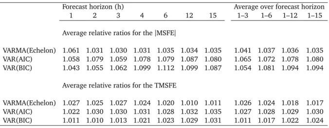
The results for the relative ratios have been plotted in Figure 2 (we present the actual values in Table 3in Appendix C). A first look at the two plots indicates that for all forecast horizons, and for both the|MSFE|and the TMSFE, the relative ratio measures are constantly greater than one. A
Figure 2: Average relative ratios for canonical Echelon form VARMA models andVARs with the lag length chosen byAICandBICover canonicalSCM VARMAmodels
Forecast horizon (h) 2 4 6 8 10 12 14 1.00 1.02 1.04 1.06 1.08 1.10 1.12 ● ● ● ● ● ● ● ● ● ● ● ● ● ● ● |MSFE| Forecast horizon (h) 2 4 6 8 10 12 14 1.00 1.01 1.02 1.03 1.04 ● ● ● ● ● ● ● ● ● ● ● ● ● ● ● TMSFE ● VARMA(Echelon) VAR(AIC) VAR(BIC)
relative ratio greater than one shows that for that forecast horizon, the scalar component VARMA models forecast better on average than the competing models. For example, for forecast horizon h=6−steps ahead, the SCM VARMA models improve on the|MSFE|(i.e., produce a lower|MSFE|) than the Echelon form VARMA models and the VARs selected by AIC and BIC by 3.5, 7.9 and 11.2 percent, respectively. The Echelon form VARMA models forecast better on average than VARs for h≥2 when considering the|MSFE|and forh≥5 when considering the TMSFE.
In Section4we conclude that a major difference between the two specifications of VARMA models is that the SCM methodology potentially identifies restrictions over and above the necessary and suffi-cient restrictions of the Echelon form. This can make SCMs more parsimonious than Echelon forms, which could be an advantage when it comes to out-of-sample forecasting. This could also have been the reason for the superior performance of the SCMs in the forecast evaluation exercise. In fact, the Echelon form methodology as presented by its various advocates (see for example Lütkepohl and Poskitt, 1996) includes an extra step which involves the elimination of any insignificant coefficients from the model viat-tests orχ2-tests to obtain optimal parsimony on the model.
We do not consider any further reduction of models here because each stage of such reductions would require a FIML estimation, which would be very time-intensive in such an extensive fore-casting exercise. Furthermore, each reduction of the parameter space must be monitored, as the Kronecker indices have to be maintained. The study of other reduction strategies that are more compatible with the procedure of identification of Kronecker indices and are more amenable to
automation, is the subject of our current research.
6 Conclusion and directions for future research
This paper provides an in-depth comparison of canonical VARMA models specified by scalar compo-nents with VARMA models specified by the Echelon form methodology. We perform this comparison at the theoretical, experimental and empirical levels. At the theoretical level we show the connection between these two forms. This has revealed the missing intuition behind the complex formulae used for specifying Echelon form models – which now eliminates using these complexities as the reason for avoiding the identification and estimation of VARMA models. Furthermore, we show that scalar component VARMA models are more flexible in the sense that their maximum “autoregressive” order does not have to be the same as the order of the “moving average” component. These orders have to be the same when specifying models via Kronecker indices in the canonical Echelon form. At the experimental level, we show, via Monte-Carlo experiments, that both of these procedures work very well in identifying some pre-specified VARMA data generating processes.
Finally, at the empirical level, the out-of-sample forecast evaluation shows that VARMA models specified by scalar components forecast better than Echelon form VARMA models, which in turn forecast better than VAR models. In the discussion of these forecast results we have acknowledged that our experimental design may have favoured the scalar component models, as there is a sense in which the Echelon form models are over-parameterised, and therefore need to be further refined. It is of interest to note that our results are consistent with the principle of parsimony, which favours models with fewer parameters as they tend to forecast more accurately than over-parameterised representations. This highlights the need for further research on refining Echelon form VARMA models.
In line with the advocates of the Echelon form, during this research we have found that its greatest advantage is its practicality in application, as we have managed to fully automate this process. This is impossible to do with the scalar component identification process, which we have managed to partly automate but which still requires a great deal of judgement and intervention from its user. Therefore, if we could find refinement processes for the Echelon form models that we are able to automate, it could lead to bringing VARMA models to the applied econometrician as it has happened with automatic univariate ARIMA modelling (see for example Mélard and Pasteels, 2000; Gómez and Maravall, 2001; Hyndman and Khandakar, 2008) and multivariate VAR modelling. Thus, a study examining alternative methods for refining the Echelon form and the effects of the refinement on the forecasting performance of VARMA models will be of great interest and is the subject of our current research.
References
Akaike, H. (1974) A new look at the statistical model identification,IEEE Transactions on Automatic Control,19, 667–674.
Akaike, H. (1976) Canonical correlation analysis of time series and the use of information criterion, in R. Mehar and D. Lainiotis (eds.)System Identification, pp. 27–96, Academic Press, New York. Athanasopoulos, G. (2007) Essays on alternative methods of identification and estimation of vector
autoregressive moving average models,unpublished PhD dissertation,Monash University, Depart-ment of Econometrics and Business Statistics.
Athanasopoulos, G. and F. Vahid (2008a) A complete VARMA modelling methodology based on scalar components,Journal of Time Series Analysis,29, 533–554.
Athanasopoulos, G. and F. Vahid (2008b) VARMA versus VAR for macroeconomic forecasting, Jour-nal of Business and Economic Statistics,26, 237–252.
Box, G. E. P. and G. M. Jenkins (1970)Time series analysis: Forecasting and control, San Francisco, California, Holden Day.
Clements, M. P. and D. F. Hendry (1993) On the limitations of comparing mean squared forecast errors (with discussions),Journal of Forecasting,12, 617–637.
Cooley, T. and M. Dwyer (1998) Business cycle analysis without much theory. A look at structural VARs,Journal of Econometrics,83, 57–88.
Dufour, J.-M. and D. Pelletier (2008) Practical methods for modelling weak VARMA processes: Iden-tification, estimation and specification with a macroeconomic application, Discussion Paper, De-partment of Economics, McGill University, CIREQ and CIRANO.
Durbin, J. (1963) Maximum likelihood estimation of the parameters of a system of simultaneous regression equations, Paper presented to the Copenhagen Meeting of the Econometric Society, reprinted inEconometric Theory,4, 159-170, 1988.
Fernández-Villaverde, J., J. F. Rubio-Ramírez and T. J. Sargent (2005) A,B,C’s (and D’s) for under-standing VARs,NBER Technical Report 308.
Fry, R. and A. Pagan (2005) Some issues in using VARs for macroeconometric research, CAMA
Working Paper Series 19/2005, Australian National University.
Gómez, V. and A. Maravall (2001) Automatic modeling methods for univariate series, in D. Peña, G. Tiao and R. S. Tsay (eds.)A Course in Time Series Analysis, John Wiley and Sons, New York., pp. 365–407.
Biometrica,56, 223–225.
Hannan, E. J. (1970)Multiple time series, John Wiley & Sons, New York.
Hannan, E. J. (1976) The identification and parametrisation of ARMAX and state space forms, Econo-metrica,44, 713–723.
Hannan, E. J. and M. Deistler (1988)The statistical theory of linear systems, John Wiley & Sons, New York.
Hannan, E. J. and L. Kavalieris (1984) Multivariate linear time series models, Advances in Applied Probability,16, 492–561.
Hannan, E. J. and J. Rissanen (1982) Recursive estimation of autoregressive-moving average order, Biometrica,69, 81–94.
Hyndman, R. J. and Y. Khandakar (2008) Automatic time series forecasting: The forecast package for R,Journal of Statistical Software,26, 1–22.
Kailath, T. (1980)Linear systems, Prentice Hall, New Jersey.
Lütkepohl, H. (1993)Introduction to multiple time series analysis, Springer-Verlag, Berlin-Heidelberg, 2nd ed.
Lütkepohl, H. and H. Claessen (1997) Analysis of cointegrated VARMA processes,Journal of Econo-metrics,80, 223–239.
Lütkepohl, H. and D. S. Poskitt (1996) Specification of Echelon-form VARMA models, Journal of Business and Economic Statistics,14, 69–79.
Makridakis, S. and M. Hibon (2000) The M3-competition: Results, conclusions and implications, International Journal of Forecasting,16, 451–476.
Mélard, G. and J. Pasteels (2000) Automatic ARIMA modelling including interventions, using time series expert software,International Journal of Forecasting,16, 497–508.
Poskitt, D. S. (1992) Identification of Echelon canonical forms for vector linear processes using least squares,The Annals of Statistics,20, 195–215.
Poskitt, D. S. (2005) A note on the specification and estimation of ARMAX systems,Journal of Time Series Analysis,26, 157–183.
Quenouille, M. H. (1957)The analysis of multiple time series, London: Charles Griffin & Company. Ravenna, F. (2007) Vector autoregressions and reduced form representations of DSGE models,
Reinsel, G. C. (1997)Elements of multivariate time series, New York: Springer-Verlag, 2nd ed. Solo, V. (1986) Topics in advanced time series analysis, in G. Del Pino and R. Rebolledo (eds.)
Lectures in Probability and Statistics, Springer-Verlag, New York.
Stock, J. H. and M. W. Watson (1999) A comparison of linear and nonlinear univariate models for forecasting macroeconomic time series, in R. F. Engle and H. White (eds.)Cointegration, Causality and Forecasting, A Festschrift in Honour of Clive W. J. Granger, New York: Oxford University Press. Tiao, G. C. (2001) Vector ARMA, in D. Peña, G. C. Tiao and R. S. Tsay (eds.)A Course in Time Series
Analysis, John Wiley and Sons, New York, pp. 365–407.
Tiao, G. C. and G. E. P. Box (1981) Modelling multiple time series with applications,Journal of the American Statistical Association,76, 802–816.
Tiao, G. C. and R. S. Tsay (1989) Model specification in multivariate time series (with discussions), Journal of the Royal Statistical Society B,51, 157–213.
Tsay, R. S. (1989) Parsimonious parametrisation of vector autoregressive moving average models, Journal of Business and Economic Statistics,7, 327–341.
Tsay, R. S. (1991) Two canonical forms for Vector ARMA processes,Statistica Sinica,1, 247–269. Tunnicliffe-Wilson, G. (1973) The estimation of parameters in multivariate time series models,
Jour-nal of the Royal Statistical Society B,35, 76–85.
Watson, M. W. (2001) Macroeconomic forecasting using many predictors, inAdvances in Economics and Econometrics, Theory and Applications, eds. M. Dewatripont, L. Hansen and S. Turnovsky, Eighth World Congress of the Econometric Society, III, 87-115.
Zellner, A. and F. Palm (1974) Time series analysis and simultaneous equation econometric models, Journal of Econometrics,2, 17–54.
A Data Generating Processes considered in Section
4.1
yt= 0.5 −0.6 0.7 0.6 0.7 −0.4 0.3 0.6 0.4 yt−1+εt (10) yt=εt− 0.5 −0.6 0.7 0.6 0.7 −0.4 0.3 0.6 0.4 εt−1 (11) 1 0 0 0.4 1 0 −0.6 0 1 yt= 0.7 0.6 0.4 0. 0. 0. 0. 0. 0. yt−1+εt− −0.7 0. 0. 0. 0. 0. 0. 0. 0. εt−1 (12) 1 0 0 0.6 1 0 0.4 0.7 1 yt = 0.5 0.6 −0.4 0.2 0.7 0.5 0 0 0 yt−1+εt− 0.5 0.7 0 0 0 0 0 0 0 εt−1 (13) 1 0 0 0.6 1 0 0.4 0.7 1 yt= 0.5 0.6 −0.4 0 0 0 0 0 0 yt−1+εt− 0.5 0.7 0 0.2 0.7 0.5 0 0 0 εt−1 (14) 1 0 0 0 1 0 0.5 −0.7 1 yt= 0.7 −0.5 0.7 0.6 0.3 0.6 0 0 0 yt−1+εt− 0.5 −0.6 0 0.6 0.7 0 0 0 0 εt−1 (15) 1 0 0 0.4 1 0 0 −0.6 1 yt = 0.7 −0.6 0.4 0.6 −0.5 −0.4 0.3 −0.6 0.4 yt−1+εt− 0.7 0.4 −0.6 0 0 0 0 0 0 εt−1 (16) 1 0 0 0. 1 0 0. 0. 1 yt= 0.6 −0.7 0.4 0.7 0.5 −0.4 0.3 −0.7 0.4 yt−1+εt− 0.7 −0.3 0.4 0.2 0.6 0.5 −0.3 0.4 0.4 εt−1 (17)B Data Summary
This appendix lists the time series that are used in this paper. The series have been directly down-loaded from Mark Watson’s web page (http://www.wws.princeton.edu/mwatson/). The names (mnemonics) given to each series have been reproduced fromWatson (2001). The superscript in-dex on the series name is the transformation code which corresponds to: (1) the level of the series, (2) the first difference ∆yt = yt−yt−1
and (3) the first difference of the logarithm, i.e., series transformed to growth rates 100∗∆lnyt
. For complete descriptions of the series refer toWatson
(2001).
(i) Output and income
IP3 IPP3 IPF3 IPC3 IPUT3 PMP1 GMPYQ3
(ii) Employment and hours
LHUR1 LPHRM1 LPMOSA1 PMEMP1
(iii) Consumption, manufacturing and retail
MSMTQ3 MSMQ3 MSDQ3 MSNQ3 WTQ3 WTDQ3 WTNQ3
RTQ3 RTNQ3 CMCQ3
(iv) Real inventories and inventory-sales ratios
IVMFGQ3 IVMFDQ3 IVMFNQ3 IVSRQ2 IVSRMQ2 IVSRWQ2 IVSRRQ2
MOCMQ3 MDOQ3
(v) Prices and wages PMCP1
(vi) Money and credit quantity aggregates
FM2DQ3 FCLNQ3
(vii) Interest rates
FYGM32 FYGM62 FYGT12 FYGT102 TBSPR1
(viii) Exchange rates, stock prices and volume
C Tables
Table 2: Percentage better counts for canonical SCM VARMA models versus canonical Echelon form VARMAmodels andVARswith the lag length chosen byAICandBIC
Forecast horizon (h)
1 2 3 4 5 6 7 8 9 10 11 12 13 14 15 Average
PB for the|MSFE|
VARMA(SCM) 30 31 30 40 40 41 49 41 50 48 45 46 45 45 44 42 VARMA(Echelon) 22 24 21 27 27 24 23 29 22 30 29 26 29 26 23 25
VAR(AIC) 27 19 26 16 19 21 13 13 14 11 13 11 9 13 14 16
VAR(BIC) 21 26 23 17 14 14 16 17 14 11 13 17 17 16 19 17 PB for the TMSFE
VARMA(SCM) 37 34 32 41 41 41 47 41 40 40 46 40 40 39 39 40 VARMA(Echelon) 22 18 16 17 21 17 19 23 29 29 27 32 30 27 23 23 VAR(AIC) 21 17 21 19 14 19 11 10 10 10 10 11 10 13 13 14 VAR(BIC) 20 31 31 23 24 23 23 26 21 21 17 17 20 21 25 23 Note: all figures have been rounded to the nearest integer
Table 3: Average relative ratios for canonical Echelon formVARMAmodels andVARswith lag length chosen byAICandBICover canonicalSCM VARMAmodels
Forecast horizon (h) Average over forecast horizon
1 2 3 4 6 12 15 1–3 1–6 1–12 1–15
Average relative ratios for the|MSFE|
VARMA(Echelon) 1.061 1.031 1.030 1.031 1.035 1.034 1.035 1.041 1.037 1.036 1.035 VAR(AIC) 1.058 1.079 1.059 1.078 1.079 1.087 1.080 1.065 1.072 1.078 1.080 VAR(BIC) 1.043 1.055 1.062 1.099 1.112 1.099 1.087 1.054 1.081 1.094 1.094
Average relative ratios for the TMSFE
VARMA(Echelon) 1.027 1.025 1.027 1.024 1.020 1.010 1.011 1.026 1.024 1.018 1.017 VAR(AIC) 1.022 1.030 1.030 1.031 1.028 1.032 1.035 1.027 1.028 1.029 1.030 VAR(BIC) 1.011 1.010 1.013 1.021 1.023 1.029 1.031 1.011 1.017 1.022 1.024