Jethro (2016) LASSO vector autoregression structures for very
short-term wind power forecasting. Wind Energy. ISSN 1095-4244 (In Press) ,
This version is available at
https://strathprints.strath.ac.uk/57829/
Strathprints
is designed to allow users to access the research output of the University of
Strathclyde. Unless otherwise explicitly stated on the manuscript, Copyright © and Moral Rights
for the papers on this site are retained by the individual authors and/or other copyright owners.
Please check the manuscript for details of any other licences that may have been applied. You
may not engage in further distribution of the material for any profitmaking activities or any
commercial gain. You may freely distribute both the url (https://strathprints.strath.ac.uk/) and the
content of this paper for research or private study, educational, or not-for-profit purposes without
prior permission or charge.
Any correspondence concerning this service should be sent to the Strathprints administrator:
strathprints@strath.ac.uk
The Strathprints institutional repository (https://strathprints.strath.ac.uk) is a digital archive of University of Strathclyde research outputs. It has been developed to disseminate open access research outputs, expose data about those outputs, and enable the
DOI: 10.1002/we
RESEARCH ARTICLE
LASSO Vector Autoregression Structures for Very Short-term
Wind Power Forecasting
L. Cavalcante1, Ricardo J. Bessa1, Marisa Reis1and Jethro Browell2
1
INESC Technology and Science (INESC TEC), Campus da FEUP, Rua Dr. Roberto Frias, 4200-465 Porto Portugal
2University of Strathclyde, Royal College Building, 204 George Street, Glasgow, Scotland
ABSTRACT
The deployment of smart grids and renewable energy dispatch centers motivates the development of forecasting techniques that take advantage of near real-time measurements collected from geographically distributed sensors. This paper describes a forecasting methodology that explores a set of different sparse structures for the vector autoregression (VAR) model using the Least Absolute Shrinkage and Selection Operator (LASSO) framework. The alternating direction method of multipliers is applied to fit the different VAR-LASSO variants and create a scalable forecasting method supported by parallel computing and fast convergence, which can be used by system operators and renewable power plant operators. A test case with 66 wind power plants is used to show the improvement in forecasting skill from exploring distributed sparse structures. The proposed solution outperformed the conventional autoregressive and vector autoregressive models, as well as a sparse-VAR model from the state of the art. Copyright c0000 John Wiley & Sons, Ltd.
KEYWORDS
Wind power; vector autoregression; scalability; sparse; renewable energy; parallel computing
Correspondence
Ricardo J. Bessa, INESC Technology and Science (INESC TEC), Campus da FEUP, Rua Dr. Roberto Frias, 4200-465 Porto Portugal. E-mail: ricardo.j.bessa@inesctec.pt
Received . . .
1. INTRODUCTION
Operating a power system with high integration levels of wind power is challenging and demands for a continuous improvement of wind power forecast tools [1][2]. Furthermore, the participation of wind power in the electricity market also requires accurate forecasts in order to mitigate financial risks associated to energy imbalances [3][4].
The recent advent of smart grid technologies will increase the monitoring capability of the electric power system [5]. Furthermore, the investment in renewable energy dispatch centers enables real-time acquisition of time series measurements from wind power plants (WPP) [6]. The availability of the most recent WPP measurements improves the forecast skill during the first lead-times, commonly calledvery short-term horizon[7].
For this time horizon, it is generally established that statistical models are more accurate than physical models, while for longer time horizons the most relevant inputs come from Numerical Weather Predictions (NWP) models [7]. Even recent advances in physical models, such as the High Resolution Rapid Refresh (HRRR) model developed by U.S.
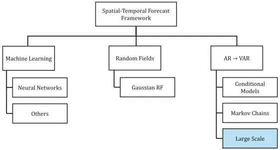
Spatial-Temporal Forecast Framework AR → VAR Conditional Models Large Scale Random Fields Gaussian RF Machine Learning Neural Networks
Others Markov Chains
Figure 1.Groups of models from the state of the art.
National Oceanic and Atmospheric Administration (NOAA), are outperformed by statistical models that use recent WPP observations [8].
In the state of the art, a broad family of statistical models are available for thevery short-term horizon. Two examples are the conditional parametric autoregression (AR) and regime-switching models that incorporate online observed local variables (i.e., wind speed and direction) to reduce the wind power forecast error for 10 min-ahead forecasting [9]. Another example is the use of automatic self-tuning Kalman filters that incorporate NWP information [10].
In this context, information from WPP time series distributed in space can be used to improve the forecast skill of each WPP. The first results were presented by Gneiting et al. for two hours-ahead wind speed forecasting [11]. The authors showed that a Regime-Switching Space-Time Diurnal model that takes advantage of temporal and spatial correlation from geographically dispersed meteorological stations as off-site predictors can have a root mean square error (RMSE) 28.6% lower than the persistence forecasts. Expert knowledge and empirical results were used to select the predictors. In [12], two additional statistical models are proposed, Trigonometric Direction Diurnal model and Bivariate Skew-T model. These results were generalized by Tastu et al. by studying the spatio-temporal propagation of wind power forecast errors [13] . The authors showed evidences of cross-correlation functions with significant dependency in lags of a few hours.
These works motivated the appearance of recent research that explores information from neighboring WPP. Figure 1 groups the state of the art methods applied to wind power by category.
The first group consists of machine learning methods, such as artificial neural networks. To the authors’ knowledge, there is little research concerning the application of machine learning models to this problem. In [14] it is described a online sparse Bayesian model based on warped Gaussian process to generate probabilistic wind power forecasts. A sparsification strategy is used to reduce the computational cost and the model includes wind speed observations from nearby WPP and NWP data. Also in this category, but applied to solar power forecasting, in [15] multilayer perceptron neural networks are used to combine measurements of neighboring PV systems, and in [16], component-wise gradient boosting is used to explore PV observations from a smart grid.
The following limitations were identified for this first group: (a) a separated model is fitted to each location, which increases the computational time; (b) the scalability of the solution decreases when the number of predictor increases; (c) with the exception of the sparse Bayesian model, the others do not provide a sparse vector of coefficients.
The second group consists of random fields. To the authors’ knowledge, the only work that explores this theory is from Wytock and Kolter [17]. The model is based on sparse Gaussian conditional random field and uses a new second-order
active set method to solve the problem. The main limitation of the method is that it requires a copula transformation in order to have a Gaussian marginal distributions, which might not solve the boundary problem of variables with limited support (e.g., wind power between zero and rated power). Moreover, the computational time for a solution with high accuracy is around 160 min for a case-study with seven WPP [18].
The third group is related to classical time series theory. Tastu et al. extended their previous work in [13] to the multivariate framework [19], i.e. from an AR to a vector autoregression (VAR) model. The VAR coefficients are allowed to vary with external variables, average wind direction in this case. The main limitation is a non-sparse matrix of coefficients since feature selection is not performed. A similar methodology was applied in [20] to generate probabilistic forecast based on geographically distributed sensors. Also in in this case, the predictors are manually selected based on cross-correlation analysis.
He et al. presents a two stages approach [21]:(1) offline spatial-temporal analysis carried out on historical data with multiple finite-state Markov chains; (2) online forecasting by feeding a Markov chain with real-time measurements of the wind turbines. Similar to previous works, different sparse structures of the spatial-temporal relations are not fully explored. The same authors in [22] propose a different approach based on VAR model fitting with sparsity-constrained maximum likelihood. The main limitation of this approach is that the sparse coefficients are not automatically defined, instead, expert knowledge and partial correlation analysis are employed.
Aiming to generate forecasts on a large spatial scale, e.g. hundreds of locations, Dowell and Pinson proposed the sparse-VAR (ssparse-VAR) approach for 5 min-ahead forecasts [23]. The ssparse-VAR method generates probabilistic forecasts based on the logit-normal distribution (see [24]), whose mean is estimated with a VAR model and variance by a modified exponential smoothing. A state-of-the-art technique from [25] is employed to fit a VAR model with a sparse coefficient matrix. The work proposed in the present paper is closely related to the sVAR and provides the following original contributions:
1. Explores a set of different sparse structures for the VAR framework using the Least Absolute Shrinkage and Selection Operator (LASSO) framework [26];
2. Applies the alternating direction method of multipliers (ADMM) [27] to fit the different VAR-LASSO variants; 3. Proposes a scalable forecasting method based on parallel computing, fast convergence optimization algorithm and
matrix calculations.
The proposed method will be compared with the sVAR approach in terms of advantages and limitations, applied to a case-study with 66 WPP located in the same control area. It should be stressed that the proposed approach is compatible with previous works from the literature. For instance, it can be used for spatial-temporal correction of forecast errors (see [13]), extended to conditional VAR (see [19]) or used to generate probabilistic forecasts based on the logit-normal distribution (see [23]).
The paper is organized as follows. Section 2 presents the different sparse structures for the VAR model. Section 3 describes the application of the ADMM method to fit the VAR model in its different LASSO variants. The test case results are presented in Section 4. Section 5 presents the conclusion and future work.
2. SPARSE STRUCTURES FOR THE VAR MODEL
The VAR model allows a simultaneous forecast of the wind generation in several neighboring sites combining time series information. However, forecasting with VAR models may be intractable for high dimensional data since the non-sparse coefficients matrix grows quadratically with the number of series included in the model. In order to overcome this limitation, in [28] it is proposed the combination of LASSO and VAR frameworks, which is further explored in this paper for very short-term forecasting of wind power.
2.1. Formulation of the Forecasting Problem
The VAR model allows us to model the joint dynamic behavior of a collection of WPPs by capturing the linear interdependencies between its time series. In this multivariate (or spatio-temporal) framework, the future trajectory of output from each WPP in the model is based on its own past values (lagged values) and the past values of the other WPPs included in the model.
Suppose yi,t is the time series containing the average power measured at WPP i and time interval t. Using an
autoregressive (AR) process of orderp(AR[p]) it is possible to describe a future trajectory based on its past observations as yi,t=µ+ p X l=1 β(l)·yi,t−l+ǫt, (1)
whereβ(1), . . . , β(p)are the model coefficients,µis a constant (or intercept) term,pis the order of the AR model, andǫt
is a contemporaneous white noise (or residuals) with zero mean and constant varianceσ2 ǫ.
Let{Yt}={(y1,t, y2,t, . . . , yk,t)′}, denote ak-dimensional vector time series. Modeling it as a vector autoregressive
process of orderp(VARk[p]), we obtain an expression relating the future observations at each of thekWPPs to the past
observations of all WPPs in the model, given by
Yt=η+ p X
l=1
B(l)·Yt−l+et, (2)
in which η is a vector of constant terms, each B(l)∈Rk×k represents a coefficient matrix related to the lagl and
et∼(0,Σe)denotes a white noise disturbance term.
In order to get a compact matrix notation, let Y = (Y1, Y2, . . . , YT) define the k×T response matrix, B=
B(1), B(2), . . . , B(p) the k×kp matrix of coefficients,Z= (Z
1, Z2, . . . , ZT) the kp×T matrix of explanatory
(or predictors) variables, in whichZt= (Yt′−1, Yt′−2, . . . , Yt′−p), andE= (e1, e2, . . . , eT)the k×T error matrix. To
simplify the notation, considerm=kp. Then it is possible to express (2) as
Y =η1′+BZ+E, (3)
with1denoting aT×1vector of ones.
The matrix of unknown coefficients needs to be correctly estimated to obtain the model that “best” characterizes the data. Commonly, this is achieved using the least squares statistical methodology by choosing the coefficients that minimize the sum of squared errors. The predictor that will be deduced gives, for a given sample, the in-sample forecasts of the variable of interest.
Usually this methodology is applied with centered variables instead of the original ones. This allows simplifications in the calculation, including the model handling without intercept term. The intercept can be easily estimated after the model has been fitted. As a result, and assuming centered variablesY andZ,ηwill no longer appear in the least squares objective function.
The multi-period forecasts can be generated with two alternative strategies, iterative or direct approach [29]. In this paper, a direct approach, in which a specific model is created for each lead-time, is adopted to generate six hours ahead wind power forecasts.
2.2. Sparse Structures with LASSO
This section presents a set of different sparse structures for the LASSO-VAR model, inspired by [30], to capture the dynamics of the underlying system.
The LASSO framework is powerful and convenient to use when handling high-dimensional data. The loss function is a regularized version of least squares that introduces anL1penalty on the coefficients. The penalty function shrink some
of the coefficients to zero, performing variable selection and producing a sparse solution. Instead of assuming that all the predictors are contributing to the model, this framework extracts the most important predictors, i.e. those with the strongest contribution to the prediction of the the target variable.
Letk.krrepresents both vector and matrixLr norms. The standard LASSO-VAR (sLV) loss function is expressed as
[30]
1
2kY −BZk
2
2+λkBk1, (4)
whereλ >0is a scalar regularization (or penalty) parameter controlling the amount of shrinkage.
TheL1penalty works as a sparsity-inducing term over the individual entries of the coefficient matrixB, zeroing some
of them in a element-wise manner.
Since the same predictors are available for each target variable (each WPP), the VAR coefficients can be estimated with ordinary least squares applied independently for the regression of each individual target variable [31]. The problem is then re-formulated for each row of the matrixY, with a different penalization parameter for each, resulting in a separable loss function for each variable.
The main advantage of this approach, here called Row LASSO-VAR (rLV), is the possibility of distributed computing, since each equation can be solved in parallel. Its loss function can be expressed as
1 2 Yi −BiZ 2 2+λ Bi 1, (5) whereYi andBi ,i= 1, . . . , k, correspond to theith
rows of theY andBmatrices, respectively.
An alternative to deal with model’s coefficients individually, which results in an unstructured sparsity pattern, is to make some simple modifications to the standard LASSO-VAR penalty in order to capture different sparsity patterns accordingly to the inherent structure of the VAR [30]. These modifications produce more interpretable models that offer great flexibility in the detection of the true underlying dynamics of the system, which is especially fruitful in the high-dimensional context. To take into account characteristics such as lag selection, within-group sparsity, delineation between a component’s own lags and those of another component and evaluate which variables add forecast improvement, the following LASSO-VAR sparse structures are explored: Lag-Group LASSO-LASSO-VAR (lLV), Lag-Sparse-Group LASSO-LASSO-VAR (lsLV), Own/Other-Group LASSO-VAR (ooLV) and Causality-Own/Other-Group LASSO-VAR (cLV). These LASSO schemes look through the sparsity in distinct group structures trying to find the ideal sparsity pattern.
The Lag-Group LASSO-VAR model considers the coefficients grouped by their time lags and looks for time lags that add forecast improvement. Its objective function is
1 2kY −BZk 2 2+λ p X l=1 B(l) 2, (6)
where eachB(l)is a sub-matrix containing the laglcoefficients.
This structure can be relevant if the interest is to perform lag selection. However, although it is advantageous when all time series tend to exhibit similar dynamics, it might be too restrictive for certain applications since all the coefficients of some lags are not considered in the prediction, and sometimes inefficient by including the entire lag if only few coefficients are significant.
In an attempt to overcome some of these limitations, the Lag-Sparse-Group LASSO-VAR model adds within-group (or lag) sparsity to the Lag-Group LASSO-VAR through the loss function
1 2kkY −BZk 2 2+ (1−α)λ p X l=l B(l) 2+αλkBk1, (7)
As can be easily seen, the Lag-Group LASSO-VAR and the standard LASSO-VAR are obtained considering α= 0
andα= 1, respectively. Here, as proposed in [30], the wihin-group sparsity is estimated based on the number of time series/variables, and set asα= 1/(k+ 1). In this sense, as the number of variables increases, the greater the group-wise sparsity and smaller the sparsity within-group. This variant allows to explore the significance of each lag and, at the same time, access the importance of each coefficient within each lag.
The Own/Other-Group LASSO-VAR model concerns with the possibility that, in many settings, the prediction of a variable is more influenced by their own past observations than by past observations of other variables. To address this question in a lag context, the coefficients of eachBlare grouped by the diagonal entries representing variable’s own lags,
and by off-diagonal entries representing cross dependencies with other variables, using the loss function
1 2kY −BZk 2 2+ √ kλ p X l=l diagB(l) 2+ p k(k−1)λ p X l=l B(l)− 2, (8) whereB(l)−={[B(l)]
ij:i6=j}. Since the groups differ in cardinality, it is necessary to weight the penalty accordingly
to avoid favoring the larger groups of off-diagonal entries.
If all time series do not share the same dynamics, one may be interested in finding which of them do. Recent studies have been addressing these question considering causal structures in multivariate series, also called Granger causality. The idea is that a time seriesyiis Granger-caused by other time seriesyjif knowing the past values ofyjhelps to improve the
prediction ofyi[32].
With the intention of learn a causal inference from the data, the Causality-Group LASSO-VAR model (see [33]) groups the coefficients by the corresponding variables (that they affect). Its loss function is
1 2kY −BZk 2 2+λ X i6=j B(1) ij B(2) ij. . . B(p) ij 2 . (9)
TheL2norm ofp−tuple of
B(l) ij
is a composite penalty that will force allpmatricesB(l)’s to share the same sparsity pattern, as can be observed in Figure 2. This structure can be useful to detect which locations can promote the forecasts at some location.
For a better understanding of the presented LASSO-VAR variants, the Figure 2 illustrates an example of corresponding generated sparsity patterns.
3. VAR MODEL FITTING
The LASSO structures described in the previous section are non-differentiable objective functions, which makes it challenging to solve since it is not possible to obtain a closed form solution. The ADMM is a recent powerful algorithm that circumvent this situation and has been successfully shown to be efficient and well suited to distributed convex optimization, in particular for solving many large-scale statistical problems [27]. The method also offers a high convergence performance that, for some problems, is comparable to recent competitive algorithms.
3.1. ADMM Framework
The ADMM framework combines the decomposability offered by the dual ascent method with the superior convergence properties of the method of multipliers, which means that problems with non-differenciable objective functions can be easily addressed and it is possible to perform a parallel optimization (topic covered in section 3.2).
Figure 2.Example of Sparsity Patterns produced by LASSO-VAR Structures.
To give an overview of the key elements of ADMM, first recall the LASSO-VAR objective function in (4) and rewrite it in ADMM form as minimize 1 2kY −BZk 2 2+λkHk1 subject to B−H= 0. (10)
Essentially, the ADMM form is obtained replicating theBvariable in theHvariable and adding an equality constraint imposing that this two variables are equal. This can be viewed as a splitting of the objective function in two distinct objective functions,f(B) = 12kY −BZk22andg(H) =λkHk1.
The augmented Lagrangian of this problem is
Lρ(B, H, W) = 1 2kY −BZk 2 2+λkHk1+W T(B −H) +ρ 2kB−Hk 2 2, (11)
whereWis the dual variable (or Lagrange multiplier) andρ >0is called the penalty parameter (or augmented Lagrange multiplier).
It is common to rewrite this Lagrangian in a scaled form by combining its linear and quadratic terms Lρ(B, H, U) = 1 2kY −BZk 2 2+λkHk1+ ρ 2kB−H+Uk 2 2− ρ 2kUk 2 2, (12)
whereU = (1/ρ)Wis the scaled dual variable associated with the constraintB=H. The last term will be ignored in the sequel since it is a constant and does not matter when dealing with minimizations.
The method of multipliers for this problem is
(Bk+1, Hk+1) := arg min B,HLρ(B, H, U k ) Uk+1:=Wk+Bk+1−Hk+1. (13)
The method of multipliers greatly improves the convergence properties over dual ascent, converging under far more general conditions. However, it is unable to address decomposition. The ADMM goes beyond decomposition issue by performing alternating minimization of the augmented Lagrangian overBandHinstead of the usual joint minimization. The ADMM algorithm for (10) consists of the following iterations
Bk+1:= arg min B 1 2kY −BZk 2 2+ ρ 2 B−Hk+Uk 2 2 (14) Hk+1:= arg min H λkHk1+ ρ 2 Bk+1−H+Uk 2 2 (15) Uk+1:=Uk+Bk+1 −Hk+1. (16) The ADMM performs minimization with respect toB(withH andU fixed), in (14), followed by minimization with respect toH(withBandU fixed), in (15), and finally it updates the scaled dual variableU, in (16).
Unlike the method of multipliers, the ADMM essentially decouples the functionsfandg, which makes it possible to exploit the individual structure of thefandgso thatB-minimization andH-minimization may be computed in an efficient and parallel manner.
The ADMM formulation for the other LASSO-VAR structures presented in Section 2.2 can be obtained by replacing the regularization term,g(H) =λkHk1, in (10) and subsequent expressions by the corresponding LASSO penalty function.
Nevertheless, this change is not trivial and several details should be taken into account for a practical implementation, which will be described in Section 3.3.
3.2. Distributed Fitting of the LASSO Structures
This section presents distributed ADMM based methods applied, by examples or by predictors, to the different LASSO-VAR structures. The main goal is to divide the initial problem into small local sub-problems and thus improve the computational performance by solving the problems in a distributed way, with each processor (or computer) handling a sub-problem.
Finding a solution to the problem of minimize the LASSO-VAR loss function, (4), involves computingBZandY Z′in a distributed manner. In this context, there are two main scenarios (see Figure 3): row block distribution and column block distribution, in whichZ is partitioned intoN row-blocks (splitting across predictors) or column blocks (splitting across examples), correspondingly.
One must choose the adequate scenario according to theZ-matrix dimension, i.e., choosing a row block distribution if it has a large number of rows and a modest number of columns, and a column block distribution otherwise. To cope with these settings, the same approach used for the sharing problem (in case of row-block distribution) and for global consensus problem (in case of column-block distribution) will be followed [27]. These scenarios are described, using the standard LASSO-VAR, in the remainder of this section. The same procedure can be followed for the other LASSO-VAR structures.
Figure 3.Row block distribution (left) and column block distribution (right).
Figure 4.Sub-block partitions.
3.2.1. Row block distribution
The matrixB is partitioned in N column-blocks asB= (B1. . . BN) with Bi∈Rk×mi, and the data matrixZ
is partitioned inN row-blocks asZ = (Z1, . . . , ZN)withZi∈Rmi×T, where PNi=1mi=m(see Figure 4). (Thus BZ=PN
i=1BiZi, i.e.,BiZican be thought of as a “partial” prediction ofY.) However, the blocks have to be carefully
constructed when using an autoregressive model. One has to be sure that all the lags are being considered in each block division/sub-problem. In this case, this is ensured partitioning first eachBandZ lag inNcolumn and row sub-blocks, respectively, and stacking the formed sub-blocks in each lag corresponding to the same order partition, in order to obtain blocks containing information of all the lags considered in the model.
This kind of procedure is especially important for the structures in which the penalty considers the division by lags, such as the Lag-Group and the Lag-Sparse-Group LASSO-VAR structures. For a 2-lag model it corresponds to gathering
Bi(1)withBi(2)andZi(1)withZi(2), to obtain each blockBiandZifori= 1, . . . N(see Figure 4). For simplification, the
notationBZk+1is used to express the meanBk+1Z.
Then, for standard LASSO-VAR, the model fitting problem (4) becomes
minimize1 2 Y − N X i=1 BiZi 2 2 +λ N X i=1 kBik1, (17)
and can be expressed in the sharing problem form as minimize 1 2 Y − N X i=1 Hi 2 2 +λ N X i=1 kBik1 subject to BiZi−Hi= 0, i= 1, . . . , N, (18)
with new variablesHi∈Rk×T. Thus, the scaled form of ADMM is Bk+1i := arg min Bi λkBik1+ ρ 2 BiZi−Hik+U k i 2 2 Hk+1 := arg min H 1 2 Y − N X i=1 Hi 2 2 +ρ 2 N X i=1 Bk+1i Zi−Hik+Uik 2 2 ! Uk+1 :=Uk+Bk+1 i Zi−Hik+1. (19)
Carrying out theH-update and using a single dual variable, the resulting ADMM algorithm is
Bik+1 := arg min Bi ρ 2 BkiZi+H k −BZk−Uk−BiZi 2 2+λkBik1 Hk+1 := 1 N+ρ Y −ρBZk+1+ρUk Uk+1 :=Uk+BZk+1 −Hk+1. (20)
EachBi-update is a LASSO problem that can be solved using ADMM by adapting (10) as
minimize 1 2 bYi−BiZi 2 2+bλkHik1 subject to Bi−Hi= 0, (21) whereYbi=BikZi+H k −BZk−Uk andbλ=λ/ρ.
3.2.2. Column block distribution
The matricesY andZare partitioned inNcolumn-blocks asY = (Y1. . . YN)andZ = (Z1. . . ZN), withYi∈Rk×Ti
andZi∈Rm×Ti, wherePNi=1Ti=T. (ThusYiandZirepresent theithblock of data and will be handled by theith
processor.) In this case, there is no need to perform a “special” construction of the blocks (partitioning the lags into sub-blocks) since all the lags are being considered in each block division/sub-problem.
Then, for standard LASSO-VAR, the model fitting problem (4) becomes
minimize 1 2 N X i=1 kYi−BiZik22+λkBik1, (22)
and can be expressed in the consensus problem form as
minimize 1 2 N X i=1 kYi−BiZik22+λkHk1 subject to Bi−H= 0, i= 1, . . . , N, (23)
with variablesBi∈Rk×mandH ∈Rk×m. Thus, the resulting ADMM algorithm for consensus is Bik+1 := arg min Bi 1 2 N X i=1 kYi−BiZik22+ ρ 2 Bi−Hk+Uik 2 2 Hk+1 := arg min H λkHk1+ N ρ 2 H−Bk+1−Uk2 2 Uk+1 :=Uk i +Bik+1−Hk+1. (24) 3.3. Practical Implementation
For a practical implementation, some aspects of the ADMM algorithm should be further discussed. Firstly, the efficient computation of B-update andH-update must be exploited. In addition, there are two parameters that need to be set: the LASSO regularization parameter, λ, and the ADMM penalty parameter,ρ. For all LASSO variants, all the primal variables are initialized to zero and the overall stopping criterion (that tests if the sequence{Bk+1}
k=0,1,2,...stabilizes
itself sufficiently to stop the algorithm) is set toBk+1−Bk/max(1,min(Bk+1,Bk))
≤ǫ, whereǫis the relative tolerance parameter. The only exception is the rLV structure, which is implemented based on the code suggested in Boyd [27] and considers a relative tolerance parameter,ǫrand an absolute tolerance parameter,ǫa.
The selection of the optimal tolerance parameters depends on the application and the algorithm used. Here, in order to choose a reasonable value for the tolerance parameters, a tradeoff between the model’s running time and its solution were conducted. In practice, for each LASSO-VAR structure, the problem was first solved with a relatively large tolerance, and after the solution process continued with a smaller tolerance value, depending on how important it is to accurately map the solution and have reduced running times.
3.3.1. B Update Step
TheB-update, i.e, the step (14), takes the form of a ridge regression (i.e., quadratically regularized least squares) problem, with analytical solution
Bk+1:= Y Z′+ρ(Hk
−Uk) ZZ′+ρI−1
. (25)
This solution is shared by all the LASSO-VAR structures presented in Section 2.2.
TheB-minimization step of the ADMM (14) reduces to solving a system of linear equations involving the matrix
ZZ′+ρI. As long as the parameterρremains constant throughout the algorithm, the factorization of the matrixZZ′+ρI
can be cached once at the outset, and subsequent iterations can be barried out cheaply only involving back-solving the system using this factorization. Furthermore, for “skinny”Zmatrices (i.e.,m≥n), one may apply the matrix inversion lemma to(ZZ′+ρI)−1
and instead compute the factorization of the smaller matrix(I+ (1/ρ)Z′Z)−1
.
In a column block distribution framework, the same technique used for (14) applies forBi-update in (24) , resulting in
the analytical solution
Bik+1:= YiZi′+ρ(H k −Uik) ZiZi′+ρI −1 . (26)
The same techniques as above, i.e. the factorization ofZZ′+ρIand the matrix inversion lemma, can also be applied to obtain an efficient method for computing multiple updates.
3.3.2. H Update Step
The H-update will result inL1−L2minimization problems that can be solved by means of shrinkages. For the standard Lasso-VAR, the solution to step (15) is given element-wise by
Hk+1=S1
whereS1is the scalarsoft thresholdingoperator, defined as S1(x, a) = x
|x|max{0,|x| −a}. (28)
The shrinkage (28) is the proximity operator of theL1norm S1(x, a) = arg min w akwk1+ 1 2kw−xk 2 2. (29)
Following the same procedure used for standard LASSO-VAR, theH-update for Row LASSO-VAR is given by
Hk+1=S1
Bik+1+Ui k, λ/ρ. (30)
For Lag-Group LASSO-VAR instead of doing scalar soft thresholding, a matrix soft thresholding is performed, i.e.,
Hk+1=S2
B(l)k+1+U(l)k, λ/ρ, (31)
whereS2is the matrixsoft thresholdingoperator, defined as S2(X, a) = X
kXk2
max0,kXk2−a . (32)
Similarly to the approach used in [34], theH-update solution for Lag-Sparse-Group LASSO-VAR, can be obtained combining scalar and matrix soft thresholding and is given block-wise by
Hk+1=S2
S1
B(l)k+1+U(l)k,(1−α)λ/ρ, αλ/ρ. (33)
For Other/Own LASSO-VAR, two vector soft thresholding are performed, one for diagonal entries and other for off-diagonal entries, in the following way
Hk+1=S2
diagB(l)k+1+U(l)k,√kλ/ρI+S2
(B(l)k+1+U(l)k)−,pk(k−1)λ/ρ(1−I), (34)
where1denotes ak×kmatrix of ones andIdenotes thek×kidentity matrix.
Finally, for Causality-Group LASSO-VAR, theH-update solution can be obtained performing a vector soft thresholding and is given row-wise by
Hk+1=S2 B(1)k+1+U(1)k ij B(2)k+1+U(2)k ij. . . B(p)k+1+U(p)k ij, λ/ρ . (35)
In the column block distribution framework, the procedure is the same but adjusting the soft thresolding operator to each LASSO-VAR structure. For instance, for the standard LASSO-VAR, the solution toH-update in (24) is given by
Hk+1=S1
Bk+1+Uk, λ/(N ρ). (36)
Further details aboutsoft thresholdingoperator can be found in [27].
3.3.3. Parameters Estimation
The optimal parameter values for each LASSO-VAR structure are estimated throughk-fold cross validation, where the pair(bλ,ρb)that gives rise to the lowest square error is selected for each lead-time.
To perform cross validation, a grid of λand ρvalues are considered. For λ, a decreasing sequence of values are computed, spaced logarithmically from the valueλmax yielding to the sparsest solution (diagonal coefficient matrices).
Theλmaxis calculated following the rule described in [33].
Selectingρas a function ofλgives a desirable performance and the computational effort appears to be smaller. Hence,
ρ=ρ∗λis assumed, withρ∗being an auxiliary constant, and a range of constant valuesρ∗is considered to perform cross
validation.
3.3.4. Computational Implementation
The ADDM algorithm can be implemented with several distributed processing systems. In [35], the technologies/platforms are classified into two types: (a) horizontal scaling that involves distributing the workload by several servers (multiple independent machines) - decentralized and distributed cluster (cloud) computing framework; (b)vertical scalingthat involves installing more processors, memory and faster hardware inside a single machine. For horizontal scaling, Message Passing Interface (MPI) was the first communication protocol to distribute and exchange the data between peers, Apache Hadoop with MapReduce as the data processing scheme emerged later, and Apache Spark is the prevalent solution. The main limitation of MapReduce is that it is not designed for iterative processes due to disk I/O limitations [35], which degrades the performance of the ADMM iterations. Spark has the unique feature to perform in-memory computations that overcomes the MapReduce limitations for iterative processes and currently is the adequate solution to implement ADMM in cluster (cloud) computing. Recent developments, such as HaLoop and Twister, seek to improve MapReduce performance for iterative tasks [36].
The most popular vertical scale up technologies are High Performance Computing Clusters (HPC), multicore processors, Graphics Processing Unit (GPU) and Field Programmable Gate Arrays (FPGA). The ADDM algorithm can be implemented in these platforms. In this paper, the ADMM was implemented in a multicore processor technology using multithreading (i.e., execute each task/sub-problem in parallel), which is available is most of the programming languages (e.g., Parallel Computing Toolbox in MATLAB and OpenMP in C/C++). It should be stressed that compared to multicore processors, GPU has a much higher number of processing cores and in [37] it is reported an implementation of the ADMM algorithm in GPU.
4. APPLICATION AND CASE STUDY
4.1. Experimental Setup 4.1.1. Dataset Description
The proposed VAR-LASSO frameworks are tested on hourly mean wind power data that comprises one year of observations from 66 WPPs located in the same control area. The individual rated power ranges between 2 MW and 220 MW. All data have been normalized by the nominal power so that its values are between 0 and 1. The time series data, as depicted in Figure 5 for two WPPs, exhibits a high cross-autocorrelation in lags different from zero and one.
The first nine months of the year (January-September) are used as a training set on which the implementation of the fitting procedure is optimized by cross-validation. The remaining three months (October-December) are then used to evaluate the performance of the models, which results are presented in Section 4.2.
In all models, two lags are used and forecasts fromt+h,h= 1, . . . ,6, i.e., six steps ahead, are considered. For a deeper visualization of the132×6549input matrixZ, forh= 1, part of it is represented as follows (the horizontal dashed line divides the two lags):
−30 −20 −10 0 10 20 30 0.0 0.1 0.2 0.3 0.4 Lag A C F WPP 48 & 53 −30 −20 −10 0 10 20 30 0.0 0.1 0.2 0.3 0.4 Lag A C F WPP 49 & 57
Figure 5.Cross-autocorrelation plot between two wind power plants.
Z= 0.0792 0.1238 0.0545 0.1584 0.1584 · · · 0.5594 0.5446 0.6584 0.7129 0.6337 0.2222 0.3796 0.4769 0.4167 0.4630 · · · 0.2269 0.2870 0.4259 0.4120 0.3935 0.2541 0.2818 0.1823 0.0276 0.0221 · · · 0.5138 0.7624 0.7790 0.5746 0.3757 .. . ... ... ... ... . .. ... ... ... ... ... 0.2727 0.3223 0.3884 0.2727 0.3140 · · · 0.0331 0.2893 0.6446 0.6281 0.3636 0.2711 0.2042 0.2359 0.3204 0.3697 · · · 0.2482 0.1849 0.1725 0.1743 0.2113 0.3294 0.3048 0.2739 0.1194 0.1840 · · · 0.2142 0.4003 0.6166 0.5485 0.1419 0.0396 0.0792 0.1238 0.0545 0.1584 · · · 0.5347 0.5594 0.5446 0.6584 0.7129 0.1713 0.2222 0.3796 0.4769 0.4167 · · · 0.2361 0.2269 0.2870 0.4259 0.4120 0.5967 0.2541 0.2818 0.1823 0.0276 · · · 0.2431 0.5138 0.7624 0.7790 0.5746 . .. ... ... ... ... . .. ... ... ... ... ... 0.1818 0.2727 0.3223 0.3884 0.2727 · · · 0.2397 0.0331 0.2893 0.6446 0.6281 0.2324 0.2711 0.2042 0.2359 0.3204 · · · 0.2254 0.2482 0.1849 0.1725 0.1743 0.2633 0.3294 0.3048 0.2739 0.1194 · · · 0.2135 0.2142 0.4003 0.6166 0.5485 .
The ADMM tolerances are presented in Table I. For the distributed LASSO-VAR algorithms, the problem is splitted into 8 subproblems. The calculations are performed on a HP with 8 Intel Core i7-2600 CPU @ 3.40 GHz processor and 8 GB of RAM and the algorithm is programmed in MATLAB R2012a.
4.1.2. State of the Art Benchmark Model
An alternative method for estimating a sparse VAR model has been proposed in [25] and is applied to very-short-term wind power forecasting in [23]. This approach, henceforth referred to as sVAR, is based on a parameter-ranking procedure to determine the sparse structure for the VAR model and maximum likelihood estimation (MLE) to estimate the parameter values. Fitting the sVAR model is a two-stage procedure. The first stage determines the temporal order,p, of the sVAR model and makes a first estimation of the sparsity structure. The second stage refines the selection of parameters made in stage one.
The sVAR is implemented here as part of our case study so that its performance may be compared to that of the proposed VAR-LASSO method.
4.2. Results and Discussion
1 2 3 4 5 6 2 3 4 5 6 7 Time Horizon (h) Improvement over AR (%) rLV sLV lLV cLV lsLV ooLV VAR
Figure 6.RMSE Improvement of the LASSO-VAR structures over AR model.
4.2.1. Forecast Accuracy
The forecasting skill of the LASSO-VAR structures is evaluated with the root mean squared error (RMSE) and mean absolute error (MAE) calculated for thet+hlead-time with the following expressions:
RM SEt+h = v u u t1 k k X i=1 b Yt+h|t−Yt+h 2 , M AEt+h = 1 k k X i=1 bYt+h|t−Yt+h . (37)
with the forecast (Ybt+h|t) made at time instanttand observed (Yt+h) value normalized by the WPP rated power.
These skill scores were calculated separately for each model using the full dataset of errors. For lead-timet+ 1, Table II shows the global RMSE and MAE scores for the six LASSO-VAR structures and also for the VAR model.
The forecast error metrics show that all the LASSO-VAR structures outperform the VAR model in terms of RMSE and MAE. As expected, the sLV and rLV exhibit very similar scores and the structure with the worst performance is the lLV. The two best scores, highlighted in bold, are achieved by cLV and ooLV structures.
The improvement of the VAR and LASSO-VAR structures over the AR model and persistence (defined asybt+h|t=ybt),
in terms of RMSE, for each lead-time is plotted in Figures 6 and 7, respectively. These plots clearly show that the cLV and ooLV structures achieve the highest improvements for all lead-times except for lead-timet+ 5whose top is led by ooLV and lsLV. Also, all the LASSO-VAR structures show better improvement than the VAR model, more pronounced after the second lead-time.
In general, the improvement over AR is higher for the first three lead-times ranging between 5.48%and 6.91%on average for the structures with the best performance (cLV and ooLV).
It is noteworthy that the rLV and sLV also have a very pleasant demeanor for all lead-times, with an improvement deviation from the best model, between 0.07% (for the first lead-time) and 0.5% (for the fifth lead-time). Another interesting conclusion is that the improvement decays with the lead-time, meaning that the spatial-temporal information is
1 2 3 4 5 6 7 8 9 10 11 Time Horizon (h)
Improvement over Persistence (%)
rLV sLV lLV cLV lsLV ooLV VAR
Figure 7.RMSE Improvement of the LASSO-VAR structures over persistence.
Figure 8.Improvement of cLV (left) and ooLV (right) over the sVAR model at each WPP for lead-timet+ 1.
more relevant for the first three lead-times and with a peak at lead-time two that corroborates the information depicted by the cross-correlation plot (Figure 5).
The improvement over persistence increases with the time horizon till lead-timet+ 4, which is the maximum value, decreasing very slightly in the remaining lead-times. As expected, the improvement over persistence is higher compared to the improvement over the AR model.
The results concerning the forecasting performance of cLV and ooLV structures against sVAR (benchmark model from the state of the art) are presented next.
The Figure 8 compares the cLV and ooLV with the sVAR model representing, for the first lead-time, the improvement over the sVAR model for each WPP. The results show that, for the first lead-time, the sVAR only has a better performance than cLV and ooLV at one WPP. Apart from that WPP, the improvement over sVAR ranges between0.08%and9.48%
for cLV and between0.17%and9.85%for ooLV. More specifically,95%of the WPP show an improvement over2%and
55%of them achieved an improvement over5%.
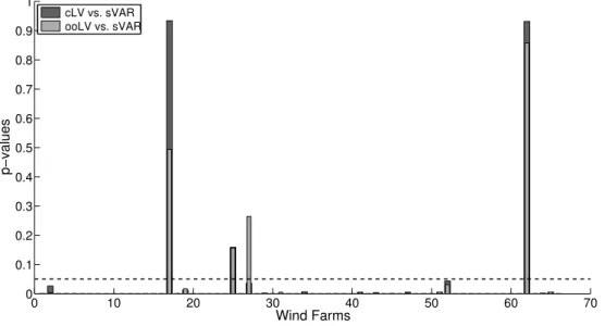
The Diebold-Mariano (DM) test [38] is applied to assess the statistical significance of the forecast error improvement in each WPP. The null hypothesis is “no difference in the accuracy of two competing forecasts”, and if thep-value is less than a significance level (i.e.,0.05in this paper), then the observed result would be highly unlikely under the null hypothesis.
0 10 20 30 40 50 60 70 0 0.1 0.2 0.3 0.4 0.5 0.6 0.7 0.8 0.9 1 Wind Farms p−values cLV vs. sVAR ooLV vs. sVAR
Figure 9.Representation of DM testp-values for forecast accuracy performance at each WPP. The dashed line represents the significance level0.05.
Time (h)
0 24 48 72 96 120 144 168 192 216 240
Wind Power (normalized)
0 0.1 0.2 0.3 0.4 0.5 0.6 0.7 0.8 0.9 1 Forecast Real
Figure 10.Real wind power generation and correspondent forecast provided by the ooLV model during ten days for the first lead-time.
Figure 9 depicts thep-values obtained for the first lead-time, which showsp-values under the significance level for the vast majority of WPP, stressing that the difference in accuracy between the competing forecasts is significant.
Finally, for illustrative purposes, a visualization of the real wind power generated and the forecast wind power output provided by the ooLV model for the first lead-time during a ten days period is shown in Figure 10 for one WPP.
4.2.2. Analysis of the Sparsity Patterns
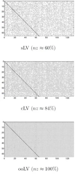
In order to understand the joint dynamic behavior of this group of WPP, the sparsity patterns (i.e., coefficients’ matrix) obtained by the LASSO-VAR structures and sVAR for the first lead-time are depicted in Figure 11. The darker shade represents coefficients that are larger in magnitude.
The figures show that the models that result in an unstructured sparsity pattern (rLV and sLV) give rise to the most sparse matrices, with about40%of null values. Immediately afterwards, with25%of sparsity, is the lsLV which has a structured blockwise sparsity, but with unstructured sparsity within each block. The structured cLV gives rise to nearly
16%of sparsity, revealing that, in average, about 11 sites were not considered to the forecast of each WPP.
Both lLV and ooLV structures present non-sparse coefficient matrices. This means that both lags (in lLV) and both diagonal and non-diagonal entries (in ooLV) were considered relevant in the model. However, while the lLV accounts for the same penalty for each lag, the ooLV assign different penalties to the diagonal and non-diagonal entries. This might justify the good performance of the ooLV, that, in general, produces non-diagonal coefficients of smaller magnitude than the ones produced by lLV. As expected, it can be observed that all figures agree that the diagonal coefficients of the first lag should have a higher magnitude, revealing that a variable’s own first lag are more likely to improve the forecast than the other entries.
The top performance of ooLV highlights the great importance of the predictors corresponding to the first lag in the prediction, relatively to the remaining coefficients, that should also be taken into account but with a smaller contribution. Also, the good results obtained by cLV demonstrates the importance of learning the causal inference from the data in order to find out which are the locations that add improvement to the prediction.
The sparsity obtained by the sVAR model (around96%) is much higher than the one obtained by any of the LASSO-VAR structures and it is possible to distinguish a great prevalence of the diagonal entries compared with the non-diagonal entries. However, a higher sparsity does not always indicate a better performance and other aspects, such as forecast improvement and computational time, should be considered when choosing the most appropriate model for each case.
4.2.3. Computational Performance
In this subsection the computational performance of the distributed ADMM algorithm is assessed. Since the input matrix has a modest number of rows and a large number of columns (Z∈R132×6549for first lead-time), a column block distribution scenario is followed. In the implementation of the distributed algorithm, the B-update and U-update are performed in parallel.
The skill scores obtained for each ADMM-based distributed LASSO-VAR algorithm are very similar to the corresponding non-distributed version. Consequently, the running times and number of iterations of both distributed and non-distributed versions are evaluated and compared to investigate which advantages one may enjoy when a parallel computation is performed.
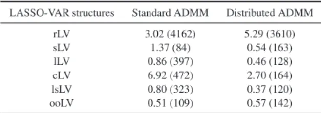
The results are depicted in Table III that shows that the use of distributed ADMM results in a decrease of the running time for all structures except for the rLV and ooL, and in a decrease of the iteration number for all structures except sLV and ooLV.
To properly analyze these results, the computational times are separated to distinguish the time elapsed in the cycle where the iterations are made and the time elapsed out of this cycle where auxiliary calculations, such as the Cholesky factorization, are performed. As one knows, the running time of each cycle depends on the number of iterations taken, then it is more appropriate to display the time that each structure takes to perform one iteration, i.e., a per iteration cost, in order to make the algorithms comparable. The running times for each structure, using both versions of the ADMM (distributed and non-distributed), by iteration and for auxiliary calculations, are represented in Figure 12.
Concerning the time by iteration, it is possible to note that all structures show very similar results in both versions, except the sLV in which the running time is greatly reduced when a distributed version is used. As a result, the decreasing of the total running time for all structures, except for sLV, is very sensitive to the number of iterations taken in the distributed version. This seems to justify the results in Table III relating to the structures sLV, lLV, cLV, lsLV and ooLV, taking into
Figure 11.Coefficients matrix (sparsity structure) of the different LASSO-VAR structures for first lead-time (nz =%of non-zero entries).
account that the time spent out of the cycle is similar in both versions. Also, it can be observed that the time spent by rLV out of the cycle greatly increases in the distributed version highlighting the impact of the increasing number of calculations
Figure 12.Running times by iteration (left) and outside cycle (right) of the LASSO-VAR structures using distributed and non-distributed ADMM.
(proportional to the number of WPPs) in this structure since it is applied to predict each location separately. This explains that, although the number of iterations is slightly decreased in this structure, the total elapsed time has increased.
Taking a deeper look over the fitting times of the non-distributed versions of the structures with better performances, we observe that the cLV is quite slow, possibly due to the combination of a high number of iterations with a high per iteration time, while ooLV stands out as the fastest. Although not at the top performances and of being the most time-consuming by iteration, the sLV also offers good results and its fast convergence results in a relatively low fitting time. Thereafter, if the objective is to find a model with a good performance and a low running time, the best choice should lie with the ooLV.
Regarding now the distributed versions, the rLV should not be considered since there is no advantage in its application. It is important to point out that, except the sLV, all the other structures have similar per iteration times in both versions indicating that the implementation of its distributed version only brings advantage if the number of iterations in this version is less than the one achieved in the non-distributed version. To deal with this, the tolerance of the termination criterion must be chosen with some caution. The sLV structure is the only one that shows a significant decrease in the time per iteration, getting a competitive total running time despite the number of iterations be higher. Accordingly, if one looks for a balance between the performance, the running time and the scalability, the sLV is probably the more adequate choice.
Finally, it is important to emphasize that the proposed methodology provides higher computational performance compared to competitive models (such as the sVAR, with a running time of about 39 hours), which is a key requirement for the large-scale application of the method.
5. CONCLUSIONS
This paper describes a forecasting technique that combines VAR and several variants of the LASSO framework to fully explore information from wind power time series distributed in space. The proposed methodology explores competing sparse structures for the VAR coefficients matrix and uses the ADMM optimization framework to guarantee fast convergence and parallel computation.
For a real case study with 66 wind power plants, all the different sparse structures of the LASSO-VAR model shows a better performance than the Persistence, AR and VAR models, and a sparse-VAR method from the state of the art. The Own/Other-Group LASSO-VAR (ooLV) and standard LASSO-VAR (sLV) structures turn out to be the best choices for, respectively, non-distributed and distributed implementations.
It is important to stress that one of the goals is to estimate a sparse matrix in which only the relevant predictors are selected to contribute for the forecasts with a small computational effort. However, the sparsity of the matrix depends on the number of relevant variables under the dynamic behavior considered by the structure and a more sparse matrix does not always mean better performance. For instance, it is interesting to note that the ooLV does not produce a sparse matrix of coefficients, but its results stand out in terms of both forecasting skill and computational time.
As we have shown, the skill of the LASSO-VAR structures depends on the dynamic behavior of the data and there is not a uniformly best structure. Therefore, each case must be carefully explored and sometimes a trade-off between the computational expense and predictive performance must be made in order to choose the LASSO-VAR structure that meets our objectives.
This work was motivated by the desire to explore different sparse structures and propose a forecasting solution with high scalability. Despite the focus in point forecast, this methodology can be directly applied to forecast the mean and variance of a logit-normal distribution and generate probabilistic forecasts. Future work should explore alternatives to the ADMM algorithm (e.g., coordinate descent algorithm), include exogenous variables in the VAR and consider the possibility of a dynamic sparse structure.
Finally, the forecasting skill improvement is valuable for different Transmission and Distribution System Operators (TSO and DSO) operational planning tasks. In this framework, TSO can improve the Intra-Day Congestion Forecast (IDCF, see [39]) by combining spatial-temporal nodal feed-in generation and load at the transmission network level collected by the real-time SCADA, as well as to increase renewable resources integration and reduce system costs against uncertainty (see [40] for unit commitment and economic dispatch results). For DSO, improved accuracy and the possibility of updating forecast data regularly has a positive impact in voltage control functions with PV power electronic inverters and On Load Tap Changer (OLTC) transformers, showed in [41] to mitigate voltages violations and minimize the total losses. Moreover, renewable energy traders can decrease their imbalance costs and the ADMM algorithm can be extended to construct data privacy-preserving distributed learning where several power plants collaborate to improve their forecasts without having to exchange actual generation data (see [42]). A functional requirement for all end-users is the access to power observations in some specific times during the operation day, where a data update rate between 10 and 60 minutes in the ideal solution. This defines some requirements for communication latency and bandwidth.
t
ACKNOWLEDGEMENTS
This work was made in the framework of the SusCity project (contract no. “MITP-TB/CS/0026/2013”) financed by national funds through Fundac¸˜ao para a Ciˆencia e a Tecnologia (FCT), Portugal. Jethro Dowell is supported by the University of Strathclyde’s EPSRC Doctoral Prize, grant number EP/M508159/1.
REFERENCES
1. Wang J, Botterud A, Bessa R, Keko H, Miranda V, Akilimali J, Carvalho L, Issicaba D. Wind power forecasting uncertainty and unit commitment.Applied EnergyNovember 2011;88(11):4014–4023.
2. Bessa R, Moreira C, Silva B, Matos M. Handling renewable energy variability and uncertainty in power systems operation.Wiley Interdisciplinary Reviews: Energy and EnvironmentMarch/April 2014;3(2):156–178.
3. Botterud A, Wang J, Zhou Z, Bessa R, Keko H, Akilimali J, Miranda V. Wind power trading under uncertainty in LMP markets.IEEE Transactions on Power SystemsMay 2012;27(2):894–903.
4. Gonz´alez-Aparicio I, Zucker A. Impact of wind power uncertainty forecasting on the market integration of wind energy in spain.Applied EnergyDecember 2015;159:334–349.
5. Colak I, Fulli G, Sagiroglu S, Yesilbudak M, Covrig CF. Smart grid projects in Europe: Current status, maturity and future scenarios.Applied EnergyAugust 2015;152:58–70.
6. Estanqueiro A, Castro R, Flores P, Ricardo J, Pinto M, Rodrigues R, Lopes JP. How to prepare a power system for 15% wind energy penetration: the Portuguese case study.Wind EnergyFebruary 2008;11(1):75–84.
7. Monteiro C, Bessa R, Miranda V, Botterud A, Wang J, Conzelmann G. Wind power forecasting: state-of-the-art 2009.
Technical Report ANL/DIS-10-1, Argonne National Laboratory November 2009.
8. Silva C, Bessa R, Pequeno E, Sumaili J, Miranda V, Zhou Z, Botterud A. Dynamic factor graphs - a new wind power forecasting approach.Technical Report ANL/ESD-14-9, Argonne National Laboratory September 2014.
9. Gallego C, Pinson P, Madsen H, Costa A, Cuerva A. Influence of local wind speed and direction on wind power dynamics - application to offshore very short-term forecasting.Applied Energy2011;88:4087–4096.
10. Poncela M, Poncela P, Per´an JR. Automatic tuning of kalman filters by maximum likelihood methods for wind energy forecasting.Applied Energy2013;108:349–362.
11. Gneiting T, Larson K, Westrick K, Aldrich MGE. Calibrated probabilistic forecasting at the Stateline Wind Energy Center: The regime-switching space-time method.Journal of the American Statistical Association2006;101:968–
979.
12. Hering AS, Genton MG. Powering up with space-time wind forecasting. Journal of the American Statistical AssociationMarch 2010;105(489):92–103.
13. Tastu J, Pinson P, Kotwa E, Madsen H, Nielsen HA. Spatio-temporal analysis and modeling of short-term wind power forecast errors.Wind Energy2011;14(1):43–60.
14. Kou P, Gao F, Guan X. Sparse online warped gaussian process for wind power probabilistic forecasting.Applied EnergyAugust 2013;108:410–428.
15. Vaz A, Elsinga B, van Sark W, Brito M. An artificial neural network to assess the impact of neighbouring photovoltaic systems in power forecasting in Utrecht, the Netherlands.Renewable EnergyJanuary 2016;85:631–641.
16. Bessa R, Trindade A, Miranda V. Spatial-temporal solar power forecasting for smart grids.IEEE Transactions on Industrial InformaticsFebruary 2015;11(1):232–241.
17. Wytock M, Kolter JZ. Large-scale probabilistic forecasting in energy systems using sparse gaussian conditional random fields.Proceedings of the IEEE 52nd Annual Conference on Decision and Control (CDC), Firenze, Italy, 2013.
18. Wytock M, Kolter JZ. Sparse gaussian conditional random fields: Algorithms, theory, and application to energy forecasting. International Conference on Machine Learning (ICML 2013). JLMR Workshop and Conference Proceedings, vol. 28, Atlanta, USA, 2013.
19. Tastu J, Pinson P, Madsen H. Multivariate conditional parametric models for a spatio-temporal analysis of short-term wind power forecast errors.Proceedings of the European Wind Energy Conference (EWEC 2010), Warsaw, Poland, 2010.
20. Tastu J, Pinson P, Trombe PJ, Madsen H. Probabilistic forecasts of wind power generation accounting for geographically dispersed information.IEEE Transactions on Smart GridJanuary 2014;5(1):480–489.
21. He M, Yang L, Zhang J, Vittal V. A spatio-temporal analysis approach for short-term forecast of wind farm generation.
IEEE Transactions on Power SystemsJuly 2014;29(4):1611–1622.
22. He M, Vittal V, Zhang J. A sparsified vector autoregressive model for short-term wind farm power forecasting.
Proceedings of the 2015 IEEE Power & Energy Society General Meeting, Denver, CO, USA, 2015.
23. Dowell J, Pinson P. Very-short-term probabilistic wind power forecasts by sparse vector autoregression. IEEE Transactions on Smart GridMarch 2016;7(2):763–770.
24. Pinson P. Very-short-term probabilistic forecasting of wind power with generalized logit-normal distributions.Journal of the Royal Statistical Society: Series C (Applied Statistics)August 2012;61(4):555–576.
25. Davis RA, Zang P, Zheng T. Sparse vector autoregressive modelling 2012. ArXiv:1207.0520.
26. Tibshirani R. Regression shrinkage and selection via the lasso.Journal of the Royal Statistical Society: Series B (Statistical Methodology)1996;58(1):267–288.
27. Boyd S, Parikh N, Chu E, Peleato B, Eckstein J. Distributed optimization and statistical learning via the alternating direction method of multipliers.Foundations and Trends in Machine Learning2011;3(1):1–122.
28. Hsu NJ, Hung HL, Chang YM. Subset selection for vector autoregressive processes using LASSO.Computational Statistics and data AnalysisMarch 2008;52(7):3645–3657.
29. Taieb SB. Machine learning strategies for multi-step-ahead time series forecasting. PhD Thesis, Universit Libre de Bruxelles, Belgium 2014.
30. Nicholson WB, Matteson DS, Bien J. Structured regularization for large vector autoregression.Technical Report, Cornell University September 2014.
31. Davidson R, MacKinnon J.Econometric Theory and Methods. Oxford University Press: New York, 2003. 32. L¨utkepohl H.New Introduction to Multiple Time Series Analysis. Springer: Berlin/New York, 2005.
33. Songsiri J. Sparse autoregressive model estimation for learning granger causality in time series.Proceedings of the 38th IEEE International Conference on Acoustics, Speech, and Signal Processing (ICASSP), Vancouver, BC, Canada, 2013.
34. Chartrand R, Wohlberg B. A nonconvex ADMM algorithm for group sparsity with sparse groups.Proceedings of IEEE International Conference on Acoustics, Speech, and Signal Processing (ICASSP), Vancouver, BC, Canada, 2013.
35. Singh D, Reddy CK. A survey on platforms for big data analytics.Journal of Big DataOct 2014;2(8):1–20.
36. Liu X, Wang X, Matwin S, Japkowicz N. Meta-mapreduce for scalable data mining.Journal of Big DataJuly 2015;
2(14):1–23.
37. Lebert J, Kunneke L, Hagemann J, Kramer SC. Parallel statistical multi-resolution estimation. arXiv preprint arXiv:1503.03492March 2015; .
38. Diebold F, Mariano R. Comparing predictive accuracy. Journal of Business and Economic StatisticsJuly 1995;
13(3):253–263.
39. Hanneton V, Margotin T, Nerin G, Lefebvre H. French TSO operational voltage risk management in a volatile electrical environment.Water and Energy InternationalMay 2016;59(1):1–11.
40. Xie L, Gu Y, Zhu X, Genton MG. Short-term spatio-temporal wind power forecast in robust look-ahead power system dispatch.IEEE Transactions on Smart GridJanuary 2014;5(1):511–520.
41. Ziadi Z, Oshiro M, Senjyu T, Yona A, Urasaki N, Funabashi T, Kim CH. Optimal voltage control using inverters interfaced with PV systems considering forecast error in a distribution system.IEEE Transactions on Sustainable EnergyApril 2014;5(2):682–690.
42. Pinson P. Introducing distributed learning approaches in wind power forecasting. International Conference on Probabilistic Methods Applied to Power Systems (PMAPS 2016), Beijing, China, 2016.
Table I.Tolerance parameters used for all the ADMM-based LASSO-VAR algorithms (distributed and non-distributed) rLV sLV lLV cLV lsLV ooLV VAR
Non-Distributed ǫa=1e-4;ǫr=1e-2 1e-5 1e-4 1e-5 3e-6 1e-4 1e-5 Distributed ǫa=1e-4;ǫr=5e-2 2e-3
Table II.Average RMSE and MAE (two lowest values in bold) across all sites for lead-timet+ 1(values normalized by rated power) rLV sLV lLV cLV lsLV ooLV VAR
RMSE 11.1406 11.1387 11.1979 11.1310 11.1691 11.1300 11.2281 MAE 7.5650 7.5636 7.6431 7.5538 7.6258 7.5368 7.6563
Table III.Total running times (in seconds) and number of iterations (between parenthesis) for 6 lead-times of the LASSO-VAR structures using distributed and non-distributed ADMM
LASSO-VAR structures Standard ADMM Distributed ADMM rLV 3.02 (4162) 5.29 (3610) sLV 1.37 (84) 0.54 (163) lLV 0.86 (397) 0.46 (128) cLV 6.92 (472) 2.70 (164) lsLV 0.80 (323) 0.37 (120) ooLV 0.51 (109) 0.57 (142)