Entity Matching on Unstructured Data:
An Active Learning Approach
Ursin Brunner and Kurt Stockinger
ZHAW Zurich University of Applied Sciences, Switzerland
Abstract—With the growing number of data sources in en-terprises, entity matchingbecomes a crucial part of every data integration project. In order to reduce the human effort involved in identifying matching entities between different database tables, typically machine learning algorithms are applied. Moreover, active learning is often combined with supervised machine learning methods to further reduce the effort of labeling entities as true or false matches. However, while state-of-the-art active learning algorithms have proven to work well on structured data sets, unstructured data still poses a challenge in entity matching. This paper proposes an end-to-end entity matching pipeline to minimize the human labeling effort for entity matching on unstructured data sets. We use several natural language processing techniques such assoft tf-idf to pre-process the record pairs before we classify them using a novel Active Learning with Uncertainty Sampling (ALWUS)algorithm. We designed our algorithm as a plugin system to work with any state-of-the-art classifier such as support vector machines, random forests or deep neural networks. Detailed experimental results demonstrate that ourend-to-end entity matching pipeline clearly outperforms comparable entity matching approaches on an unstructured real-word data set. Our approach achieves significantly better scores (F1-score) while using 1 to 2 orders of magnitude fewer human labeling efforts than existing state-of-the-art algorithms.
I. INTRODUCTION
Almost every company needs to integrate data from different sources to gain potentially new insights into the data. Assume, for instance, a company needs to merge information from a customer database in Zurich and another customer database in San Francisco. While one database focuses on the customers’ financial transactions, the other one provides information about their browsing patterns in a web shop. In order to analyze the customers’ behavior and predict future purchases, we need to match the customers, i.e. the entities of the two data sources. This problem is known as the Entity Matching problem. The goal is to determine if two entities refer to the same real-world object [5]. If the two data sources contain a shared unique identifier (e.g. a taxpayer number), the entity matching problem becomes as trivial as a database join. However, such unique identifiers are rare and often subject to privacy concerns.
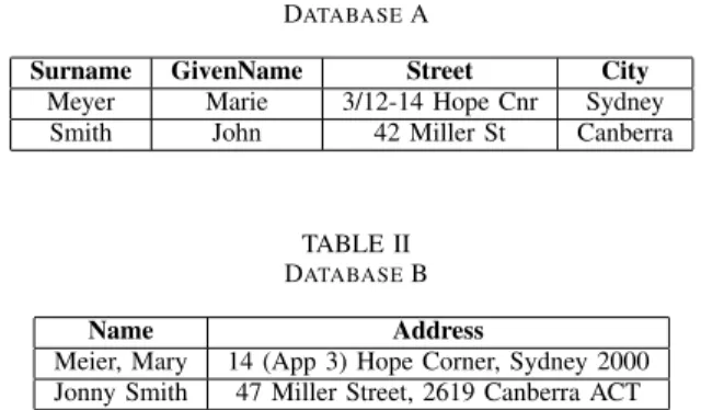
As a consequence, a data matching problem more often looks like the example shown in Tables I and II. We need to match two entities based on attributes like names, addresses or product information while dealing with various formats and differing, missing or wrong values. Given this uncertainty, the major challenge of entity matching is to identify which existing real entity pairs have the highest probability of being a match. We can thus formulate parts of end-to-end entity
matching process as a classification problem where we need to minimize the number of false positives.
TABLE I DATABASEA
Surname GivenName Street City
Meyer Marie 3/12-14 Hope Cnr Sydney Smith John 42 Miller St Canberra
TABLE II DATABASEB
Name Address
Meier, Mary 14 (App 3) Hope Corner, Sydney 2000 Jonny Smith 47 Miller Street, 2619 Canberra ACT
While early entity matching was heavily used in the health sector and in national censuses [5], it is now a challenge that appears in numerous application domains. As large companies produce (and consume) more and more data which originates from multiple data sources, the process of data integration
and data cleaning becomes crucial. In the process of data integration, entity matching is a key step, while in data cleaning, duplicate detection is of great importance.
Thecontributions of our paper are as follows:
• We introduce a novel entity matching algorithm called
Active Learning with Uncertainty Sampling (ALWUS)as core of our end-to-end entity matching pipeline. The algorithm works as a plugin system, where the learner can be replaced by any state-of-the-art classifier. • We provide deep insights into the entity matching
pro-cess, especially into the steps prior to classification. We use several natural language processing techniques such
soft tf-idf to pre-process the record pairs and to optimize theend-to-end entity matching pipeline.
• The experimental results demonstrate that ourend-to-end entity matching pipelinewith ALWUS is superior to state-of-the-art algorithms working on a real-world benchmark data set. Our approach achieves significantly better scores (F1-score) while using 1 to 2 orders of magnitude fewer human labels than existing state-of-the-art algorithms [8], [10], [15].
II. THEENTITYMATCHINGPROBLEM
In this section we first give an overview of the end-to-end process for entity matching and afterwards discuss different similarity measures to match two entities.
A. The End-to-End-Process
The process of entity matching as defined by [5] can roughly be divided into the following major steps: The first step,data pre-processing, is to clean and standardize the data. The basic idea is to ensure that the attributes used for the matching have the same structure, and their content follows the same formats. The goal of the second step, indexing or blocking, is to reduce the computational effort when comparing record pairs, i.e. records from two different data sets. Imagine dealing with two data sources ofnandmrecords. By building record pairs, we end up with a quadratic problem of size O(nm). If we now apply a string similarity measure such as theLevenshtein
distance [12], whose computational complexity is quadratic in the number of input records, the entity matching problem soon becomes computationally unfeasible. With indexing/blocking
we therefore try to apply ”cheap” and highly tolerant similarity measures to filter out those record pairs that are ”obvious” non-matches. However, the blocking step is always a trade-off between not loosing matching record pairs and computational effort.
The third step,record pair comparison, is about comparing two records in detail. In this step, only those entities are inspected, that are not pruned by the indexing or blocking step. In this step, different similarity measures are applied to identify matching entities (see Section II-B for details).
The final step, classification, decides if a record pair is a
match or a non-match. The complexity of the classifier can range from a simple threshold-based rule system to a complex active learning scenario with support vector machines or deep neural network learners as we show in this paper.
B. Similarity Measures
In this section we will discuss generic similarity measures to identify if two entities match.
String Similarities: The easiest way to compare record pairs is to consider each field of the record as a string and to apply string similarity algorithms. One of the most commonly used string comparison algorithms is theLevenshtein distance
[12]. This approximate string matching approach typically works well for comparing short strings where usually only small differences are expected. A more specialized similarity algorithm is, for instance, the Jaro-Winkler [6] algorithm, which has been designed specifically for the comparison of names.
Document Similarities: In order to match longer texts, a common approach is to use tf-idf [14] (term frequency - inverse document frequency). To compare the similarity between two records, one typically uses the cosine similarity. However, one drawback of the original tf-idf cosine similarity is the fact that it only finds exact matches. A method to resolve this issue is the soft tf-idf [14].
The basic idea of soft tf-idf is to enable fuzzy matching. Assume we have a record pair consisting of the two recordsRi
andRj, whereRi andRj are vectors with one value for each
unique term. Each term is represented by its tf-idf weights:
Ri = [wi,1, wi,2, wi,3, ...] and Rj = [wj,1, wj,2, wj,3, ...].
Before we multiply the tf-idf weights of the vectorsRiandRj
(as is common for the traditional tf-idf), we create a so called
similarity map. Next, we calculate the similarity between all the terms inRiandRj. If the similarity between two terms is
above a certain threshold (sim(terma,k, termb,k)> θ), they
are added to the similarity map.
When we later calculate the cosine similarity, we do not only multiply the two tf-idf weights, but also the similarity calculated for the similarity map. The new equation to calcu-late the cosine similarity looks as follows:
sims tf idf(Ri, Rj) =
P|sim map|
k=1 simi,k∪j,k·wi,k·wj,k
q Pn k=1w2i,k q Pn k=1wj,k2 (1) where the numerator consists only of elements whose simi-larity threshold is aboveθ. The denominator, on the other hand, contains all terms in Ri and Rj. In summary, the additional
softfeature enables us to decide at which similarity threshold
θ we consider two terms to be similar.
III. ALWUS (ACTIVELEARNING WITHUN-CERTAINTY
SAMPLING
In this section we will focus on the last step of the entity matching process, namelyclassification. Moreover, we introduce our algorithm ALWUS (Active Learning with Un-certainty Sampling).
This classification step is often performed using various supervised machine learning algorithms that require training data. However, training data for entity matching processes are often hard to obtain, which makes classical machine learning challenging. Active learning, where a learner gets only very little initial labeled data and asks then an oracle for specific further training data, has been proven to be a good alternative [1], [2], [10]. The goal of active learning is to reduce the manual labeling effort as much as possible by querying the oracle only for the most ”important” unlabeled training data. The challenge of active learning is to find the most important unlabeled training data items.
A. ALWUS - The Big Picture
ALWUS is based on the theory of active learning by un-certainty, more precisely on the idea ofQuery by Committee, which has been introduced 1992 bySeung et al.[13]. The idea of querying by committee in combination with bagging(the machine learning technique based on bootstrapping) is by now a standard active learning approach and has been successfully used in many recent works [9], [10].
The novelty in our approach is the integration of ALWUS in an end-to-end entity matching pipeline. The improvements in
pre-processingandrecord pair comparison(see Section II-B), massively speed up the learning rate of ALWUS which leads to a significant reduction of label requests to the oracle.
The intuition of our approach is as follows:
1) We start by initially labeling a few random data samples and add them to thelabeled training set.
2) Next webootstrapfrom this data and create individual training sets for each of the N learners in the learner ensemble. We train each learner on its training set. 3) As a next step, we use the learner ensemble to predict
all unlabeled data (unlabeled pool). The predictions will be different, as every learner in the ensemble has been trained on a different training set.
4) For every prediction, we calculate the empirical vari-ance in the learner ensemble. The variance is in this setup equivalent to uncertainty.
5) The uncertainty ranker uses this measure to decide which labels to query next.
6) The query is answered by an oracle. In reality, this oracle is often a human, while in a test setup the oracle is a predefined dictionary.
7) The newly labeled data is added to thelabeled training setand the active learning starts again.
B. ALWUS - The Details
We will now describe the major steps of our approach ALWUS in more detail.
1) Bootstrapping: The bootstrap [4] is a universal and powerful method that can be used to quantify the uncertainty (in terms of bias, variance and confidence intervals) associated with a given statistical estimator (learner)γ. The method does not rely on a particular data distribution and falls in the broader class of re-sampling methods [4].
Let x1, ..., xn be (possibly multivariate) realizations of
independent and identically distributed random variables X1,
X2, ...,Xn. Further assume that
b
γ=bγ(x1, ..., xn)
is an estimator of some quantity γ. We now span up a bootstrap with B estimators as follows:
1) Choose a (large) numberB ∈N
2) For b= 1, ..., B
• Drawnsamples{x∗
1, ..., x∗n}from{x1, ..., xn}with
replacement.
• Compute the estimatorγb∗
b =bγ(x ∗ 1, ..., x∗n)
3) The empirical distribution function F∗ of (bγ1∗, ...,bγB∗)
approximates the distribution ofbγ. Any statistical prop-erty of the estimator bγ can now be estimated by the bootstrap estimatebγ1∗, ...,bγ
∗
B.
For uncertainty sampling we are interested in the bootstrap variance, since we use it as a measure for uncertainty. With the bootstrap introduced above, we calculate the variance as follows: varB(γb) = 1 B−1 B X b=1 (bγb∗−γ∗)2 (2) with γ∗= 1 B B X b=1 b γ∗b (3)
GivenBis large enough, we get an empirical approximation of theexpected value(Equation 3) and thevariance(Equation 2).
2) Ensemble Learner & Uncertainty Ranker: We now use the bootstrap theory defined in Section III-B1 to create the two most important components in our architecture, theEnsemble Learner [16] and theUncertainty Ranker.
a) Ensemble Learner: The Ensemble Learner is a con-tainer for theB different sub-learners/estimators. From a high level perspective it works as any other classification learner: We fit a set of training samples and then predict a set of unknown samples based on the model trained in thefit step.
Internally the Ensemble Learner contains a list of sub-learners, where each learner has its own bootstrapped training set {x∗1, ..., x∗n}. Every time wefit a set of training samples
{x1, ..., xn}to theensemble learner, we first randomly create
B subsets of training samples{x∗
1, ..., x∗n} (the bootstrapping
process). We then train each sub-learner on its own training set.
When we predict a set of new, unlabeled samples, the
Ensemble Learner asks every of the B sub-learners for its prediction. As every sub-learner has been trained on a different data set (remember: we create the data sets randomly and with replacement), the learned models differ from each other and therefore also the predictions.
The Ensemble Learner then uses a simple concept of
majority votingto decide on the final prediction
pB(x) = arg max B
X
b=1
p(x,bγ∗b) (4) where p(γb∗) predicts the class label given and arg max returns the class label which appears most frequently.
In contrast to a simple learner, theEnsemble Learnerfurther provides thevarianceproperty for each predicted sample. As we deal with a binary classification (”match = 1”/”non-match = 0”) we can simplify the variance introduced in Section III-B1 to varB(x) = PB b=1p(x,γb ∗ b)∈ {1} B (1− PB b=1p(x,bγ ∗ b)∈ {1} B ) (5) wherexis the sample we predicted.
b) Uncertainty Ranker: In every step of the active learn-ing approach we deal with a set oflabeled training dataand a much larger set ofunlabeled data. We use aranker to decide which samples of the unlabeled data set to label next. The ultimate goal is to minimize the number of requested labels
and to maximize the performance (F1-score).
The Ensemble Learner enables the Uncertainty Ranker to do a prediction for all unlabeled data samples. The ranker then orders the predictions descending byvarianceand selects
N (batch size) samples with the highest variance, i.e. the
N samples the Ensemble Learner is most uncertain about. Finally, the active learning algorithm asks the oracle about the labels for theseN samples.
IV. EXPERIMENTAL RESULTS
In this section we describe our experiments on the end-to-end data matching process using the ALWUS active learning approach. The results demonstrate that our approach increased the initial end-to-end F1-score from a baseline of 40% to a fi-nal value of 81%, which outperforms all compared algorithms. We further explain how we reduced the human labeling effort by an order of 1 to 2 magnitudes compared to other state-of-the-art algorithms.
For our experiments we used the de-facto standard data set for entity matching, namely theAbt-Buyproduct data set [8]. TheAbt-Buydata set has a total size of 1,081 x 1,092 records which sums up to 1.2 million record pairs(without blocking). Out of these 1.2 million record pairs, 1,097 pairs are real matches.
In order to measure the quality of our matching algorithm, we use the F1-scoreand the human labeling effort.
F1-score: For the F1-score we use the traditional definition:
F1= 2·
precision·recall
precision+recall (6)
Note that entity matching data sets are typically highly imbalanced, i.e. they often contain a high number of non-matches and a low number of non-matches. In our case, the percentage of non-matches is 95%, while the percentage of matches is 5%.
Human Labeling Effort: The human labeling effort is measured as the number of query requests to the oracle. The objective is to minimize the score, as the human labeling effort is not only expensive but also often subject to errors [15]. The labeling effort for the initial training data also adds to this score.
All the experiments were executed on a Linux-based system running an Intel(R) Core(TM) i7 CPU with 4 cores and 8 threads. The system was equipped with 32 GB RAM.
A. Entity Matching Pipeline
Before demonstrating the results on the core of this paper (i.e. Active Learning with Uncertainty Sampling), we show how we improved several steps of the entity matching process and how much each optimization contributed to the overall F1-score. In particular, we will first focus on the steps pre-processing,blockingandrecord pair comparison. Without any of these improvements we reach abaseline F1-score of 40%. After applying all optimizations, we reach an F1-score of 81%.
Pre-Processing: By analyzing the data set Abt-Buy, we figured out that Buy product records often contain identifiers separated by a dash (e.g. ”STR-DG920”), while Abt records do not. By cleaning out these dashes and merging the two key tokens to a single identifier during pre-processing, we could increase performance (∆F1-score) by16%.
Indexing/Blocking: To reduce the record pairs from origi-nally 1,180,452 to 19,562, we used a simple blocking method based on Jaccard similarity with θ < 0.1. With this simple
blocking we reduced the amount of record pairs by98.35%, while loosing 102 of 1097 real matches (9.3%)1.
Record Pair Comparison: In the step record pair com-parisonwe improved the entity matching pipeline by finding an optimal similarity threshold for soft tf-idf. We will now describe this optimization.
Similarity Threshold (θ) for Soft tf-idf: Choosing the right threshold θ is fundamental for achieving good performance with soft tf-idf, as this parameter controls which tokens are considered to be matches. Hence, we executed a grid search
to find the optimal similarity measure in combination with the threshold parameter. In particular, we used the two similarity measures Jaro and Jaro-Winkler.
Our experimental results in Table III show the outcome of the grid search with a similarity threshold in the range of
[0.8,1[. We have chosen this range based on the optimal out-comes of grid search’s hyper parameter tuning. The top 4 rows show the results for the Jaro measure, while the bottom 4 rows show the results of the Jaro-Winkler measure. As an example for the massive impact of the hyper parameter, have a look at the performance difference between a similarity threshold 0.8 and 0.85 with the Jaro-Winkler similarity measure (third row from the bottom). The performance (F1-score) increases by 39%. We see the highest increase of the F1-score by 59% for the threshold θ of 0.95 (highlighted in bold). Note that when we further increase the thresholdθto 0.98, the F1-score only increases by 58%. In other words, further increasing the threshold reduces the F1-score.
TABLE III
EFFECT OF THE SIMILARITY THRESHOLD(θ)ON THE OVERALL PERFORMANCE(F1-SCORE)
Similarity Measure θ ∆F1-score
Jaro 0.8 0% Jaro 0.85 + 6% Jaro 0.95 + 13% Jaro 0.98 + 10% Jaro-Winkler 0.8 0% Jaro-Winkler 0.85 + 39% Jaro-Winkler 0.95 + 59% Jaro-Winkler 0.98 + 58%
As we originally used the parameter pair(J aroW inkler, 0.85)as a baseline, we could improve the performance of the F1-score by20%by increasing the threshold to 0.95. Finally, by performing additional feature engineering, we could further improve the F1-score by5%.
B. Classification
We will now discuss the experimental results of our classifi-cation algorithms. However, before diving into active learning, we need to find the upper limits of our learners. In other words, we want to find out what performance (F1-score) a 1Such a simple blocking approach obviously offers room for improvement,
which though is out of scope for this work.Christen et al.[5] describe various advanced blocking algorithms in detail. With a relatively small dataset of around one million pairs, one could even consider skipping the blocking step entirely.
passive learner can achieve when the full data set including all labels are used (see Section IV-B1). These performance values will then be the baseline for the active learning approach (see Section IV-B2).
1) Passive Learning: In the passive learning setup we used the full 19,562 comparison vectors (the record pairs after blocking), which contain 1,097 matches and 18,465 non-matches. We split the available data randomly in a 75% training and 25% test set.
For our experiments we used three different machine learn-ing algorithms with the followlearn-ing architecture and parameter settings:
• SVM: Support Vector Machine with a Radial Basis Function (RBF) kernel. The RBF kernel has been chosen for maximal learner flexibility.
• RF: Random Forest with 500 estimators. We determined these hyper parameters by hyper parameter-tuning, both manually and with scikit-learn’sExhaustive Grid Search. • Fully connected NN: Fully connected Neural Network (in Tensorflow) with the following architecture: input layer: 500 neurons with ReLU activation function; 3 hidden layers with 500, 500 and 50 neurons with ReLU activation function; output layer: 1 neuron with a sig-moid activation function and a binary cross entropy loss function. This architecture has been chosen based on hyper parameter tuning and exhaustive grid search. The resulting hyper parameters are a trade-off between maximal flexibility for the learner (high F1-score) and training run time.
For each of the three learners we executed 20 runs and measured the F1-score to identify matches and non-matches. The results in Table IV (average over 20 runs) indicate that there is no considerable difference between the different learners. They all achieve F1-scores between 80% - 82% .
TABLE IV
PASSIVE LEARNING RESULTS(AVERAGE OVER20RUNS) Learner Precision Recall F1-score SVM with RBF 0.874 0.765 0.816
Random Forest 0.840 0.765 0.800 fully connected NN 0.837 0.789 0.812
2) Active Learning: For the active learning approach, we used the fully optimized entity matching pipeline described in Section IV-A. We then implemented our algorithm Active Learning with Uncertainty Sampling (ALWUS)as described in Section III.
Among the thee machine learning algorithms that we com-pared in Section IV-B1, we selected the SVM learner. The choice of SVM learner has been made due to its low run time complexity and almost equal performance (F1-score) compared to more complex learners such as deep neural networks (see Table IV). We then combined 24 of those SVMs with anensemble learner (introduced in Section III-B2a). For performance reasons we chose the number 24, a multiple of the test machine’s logical cores which is 8.
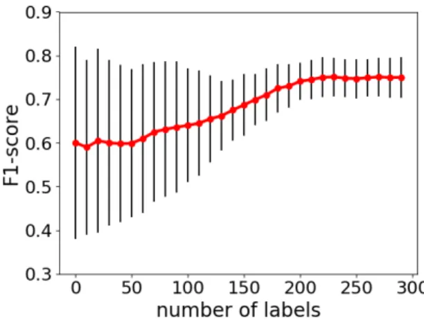
Fig. 1. Learning curve with Random Ranker over 20 runs. The red line represents an average over all runs, the black error bars indicate the variance.
The active learning process starts with aninitial training set size of only 10 records. In every iteration, the active learner requests ranked labels of 10 unknown data samples from the oracle (batch size 10). We grant the active learner a total
budget of 300 requeststo the oracle.
We will now describe the results of active learning with a Random Ranker (as the baseline) and compare it with our contribution, theUncertainty Ranker.
a) Random Ranker: As the name indicates, theRandom Ranker chooses the next label requests for the oracle at random, not considering any variance information from the learners. Figure 1 shows the average results over 20 runs. The average run starts at an F1-score of 60%, and then increases up to 75% after 230 training samples. At this point we see no further improvement until the active learner has used its full budget of 300 requests.
An interesting finding is the high variance of the scores of each single run. While the learner ensemble reaches good scores with very little training data in some runs, other runs need significantly more labels to reach a stable score. This effect is explained by the randomness of how the next label requests are chosen in a single run.
b) Uncertainty Ranker: Finally we ran active learning with the Uncertainty Ranker. While the setup stays exactly the same as with the Random Ranker, we now use a ranker that decides by the uncertainty of the learner ensemble which samples to query next. The implementation follows the theory described in Section III-A.
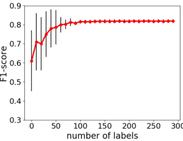
Figure 2 shows the results of an average over all 20 runs. The average run starts again at an F1-score of 60% and reaches an F1-score of 78.6% at atraining-set sizeof only 60 samples. Moreover, the algorithm reaches a stable F1-score of 81.3% after 90 samples. Afterwards the score only minimally improves until reaching the full budget of 300 requests.
We also note that the variance of the different runs is much lower when using theUncertainty Rankerthan for theRandom Ranker. After a training size of 80 samples, every run reached a minimum F1-score of at least 78%.
Fig. 2. Learning curve withUncertainty Rankerover 20 runs. The red line represents an average over all runs, the black error bars indicate the variance.
C. Comparing the Results with State-of-the-Art
TABLE V
F1-SCORES AND LABELING EFFORT FOR OUR APPROACH CALLED
ALWUS (RIGHT-MOST COLUMN)COMPARED WITH THREE STATE-OF-THE-ART ALGORITHMS.
Approach A B C ALWUS
F1-score 56% 71% 73.4% 81% Labeling effort 2,000 500 3,154 60-90 for top score
Our final results with the Uncertainty Rankers are highly encouraging. With anF1-score of 81% and higher, we score better than all compared state-of-the-art approaches as shown in Table V.
Let us analyze these results in more detail. The active learning approach of [10] reaches an F1-score of 56% on this data set (indicated as Approach A). The frameworks FEBRL and MARLIN in [8] reach a maximum F1-score of 71% (Approach B), while the hybrid approach of [15] reaches an F1-score of 73.4% (Approach C). The main reason for a superior F1-score of ALWUS is the improved pre-processing with soft tf-idf.
More important though is the improvement regarding human labeling effort. With the Uncertainty Ranker, we need only 60 - 90 samples (including initial training set) to reach an F1-score higher than 81%. We therefore reduce the human labeling effort by an order of 1-2 magnitudes compared to the state-of-the-art algorithms.
In comparison, the experiments of [10] start with an initial training set of 249 samples (F1-score of 48%). The best active learning algorithm reaches an F1-score of 56% after requesting 2,000 labels. Other active learning algorithms (e.g. CVHull [2], IWAL [3]) perform much worse in this experiment since they require almost 6,000 labeled samples to reach an F1-score
>50%.
The known entity matching systems FEBRL and MARLIN [8] both need around 500 labeled records to reach their maximum F1-scores of 71%. After 100 labels, they reach
an F1-score of roughly 20% (FEBRL), 20% (MARLIN with ADTree) and 60% (MARLIN with SVM). Note that there has been more recent work on entity matching such as [7], [11]. However, since these systems do not use an active learning approach, we cannot directly compare our results with these systems.
V. CONCLUSIONS
In this paper we proposed a novel end-to-end entity match-ing pipeline that is relevant for any data integration problem. With ALWUS we proposed an active learning algorithm with uncertainty sampling and demonstrated how to use the statis-tical theory of bootstrapping to train multiple learners with minimal training data. We created an Ensemble Learner and an Uncertainty Ranker to decide which record pairs to label next based on the uncertainty of the Ensemble Learner. Our experimental results showed how our end-to-end entity match-ing pipeline with ALWUS reached a higher F1-score (81%) than all compared state-of-the-art algorithms on a popular entity matching data set for unstructured data. Most important though, the label requests with ALWUS was 1-2 magnitudes lower than all compared state-of-the-art algorithms.
REFERENCES
[1] A. Arasu, M. G¨otz, and R. Kaushik. On active learning of record matching packages. SIGMOD, 2010.
[2] K. Bellare, S. Iyengar, A. Parameswaran, and V. Rastogi. Active sampling for entity matching with guarantees. ACM Trans. Knowl. Discov. Data, 7(3):12:1–12:24, Sept. 2013.
[3] A. Beygelzimer, S. Dasgupta, and J. Langford. Importance weighted active learning. CoRR, abs/0812.4952, 2008.
[4] R. T. Bradley Efron.An Introduction to the Bootstrap. CRC Press Book, 1994.
[5] P. Christen.Data Matching: Concepts and Techniques for Record Link-age, Entity Resolution, and Duplicate Detection. Springer Publishing Company, Incorporated, 2012.
[6] M. A. Jaro. Advances in record-linkage methodology as applied to matching the 1985 census of tampa, florida. Journal of the American Statistical Association, 84(406):414–420, 1989.
[7] P. Konda, S. Das, et al. Magellan: Toward building entity matching management systems. PVLDB, 9(12):1197–1208, 2016.
[8] H. K¨opcke, A. Thor, and E. Rahm. Evaluation of entity resolution approaches on real-world match problems. PVLDB, 3(1-2):484–493, Sept. 2010.
[9] P. Melville and R. J. Mooney. Diverse ensembles for active learning. InProceedings of the Twenty-first International Conference on Machine Learning, ICML ’04, pages 74–, New York, NY, USA, 2004. ACM. [10] B. Mozafari, Sarkar, et al. Scaling up crowd-sourcing to very large
datasets: A case for active learning. PVLDB, 8(2):125–136, Oct. 2014. [11] S. Mudgal, H. Li, et al. Deep learning for entity matching: A design
space exploration. SIGMOD, 2018.
[12] G. Navarro. A guided tour to approximate string matching. ACM Comput. Surv., 33(1):31–88, Mar. 2001.
[13] H. Sebastian Seung, M. Opper, and H. Sompolinsky. Query by commit-tee.Proceedings of the Fifth Annual ACM Conference on Computational Learning Theory, pages 287–294, 01 1992.
[14] W. W. Cohen, P. Ravikumar, and S. E. Fienberg. A comparison of string distance metrics for name-matching tasks. ACM Workshop on Data Cleaning Record Linkage and Object Identification, 2003. [15] J. Wang, T. Kraska, et al. Crowder: Crowdsourcing entity resolution.
PVLDB, 5(11):1483–1494, July 2012.
[16] C. Zhang and Y. Ma. Ensemble Machine Learning: Methods and Applications. Springer Publishing Company, Incorporated, 2012.