Advanced forecasting methods for renewable generation and loads in modern power systems

U

S

N

F

II

P

.D.

THESIS

IN

I

T

E

E

A

DVANCED

F

ORECASTING

M

ETHODS FOR

R

ENEWABLE

G

ENERATION AND

L

OADS IN

M

ODERN

P

OWER

S

YSTEMS

P

ASQUALE

D

E

F

ALCO

T

:

P

.

G

C

C

-T

:

D

.

A

B

C

:

P

.

D

R

XXX

C

S

P

S

B

D

I

E

T

’I

To Marisa and Vincenzo

i

Index

List of figures ...v

List of tables ... vii

List of abbreviations ... ix

List of symbols ... xi

Acknowledgment ... xix

INTRODUCTION ...1

CHAPTER 1. FORECASTING AND POWER SYSTEMS ...6

1.1. INTRODUCTION ...6

1.2. CLASSIFICATIONS OF FORECASTING METHODS ...7

1.3. FORECASTING METHODS APPLIED TO POWER SYSTEMS ... 11

1.3.1. Statistical approaches ... 12

1.3.1.1. Naïve approaches ... 12

1.3.1.2. Regression analysis ... 15

1.3.1.3. Univariate stochastic time series ... 16

1.3.1.4. Exponential smoothing ... 18

1.3.1.5. Bayesian approaches ... 20

1.3.1.6. Markov Chains... 21

1.3.1.7. Kalman filter ... 22

1.3.1.8. Artificial neural networks ... 23

1.3.1.9. Support vector regression ... 24

1.3.1.10. Fuzzy approaches ... 26

1.3.1.11. K-nearest neighbors ... 27

1.3.1.12. Kernel density estimation... 28

1.3.2. Physical approaches ... 29

1.3.3. Hybrid approaches ... 30

CHAPTER 2. ADVANCED PROBABILISTIC METHODS FOR SHORT-TERM PHOTOVOLTAIC POWER FORECASTING ... 33

2.1. INTRODUCTION ... 33

2.2. PROBABILISTIC METHODS FOR SHORT-TERM PHOTOVOLTAIC POWER FORECASTING: STATE OF THE ART ... 34

2.3. A NEW PROBABILISTIC BAYESIAN-BASED METHOD FOR SHORT-TERM PHOTOVOLTAIC POWER FORECASTING ... 38

2.3.1. Proposed method ... 39

2.3.1.1. Relationships that link the PV active power to the hourly clearness index and the solar irradiance ... 40

2.3.1.2. Selection of the PDFs of the hourly solar irradiance and of the hourly clearness index irradiance ... 41

ii

2.3.1.3. Exogenous linear regression model ... 43

2.3.1.4. Evaluation of the PDFs of the coefficients of the exogenous linear regression models and of the Beta distribution shape parameter ... 44

2.3.1.5. Evaluation of the samples of the predictive PDF of PV power ... 46

2.3.2. Numerical applications ... 48

2.3.2.1. Data characteristics ... 48

2.3.2.2. Assessment of the quality of forecasts ... 50

2.4. A NEW PROBABILISTIC ENSEMBLE METHOD FOR SHORT-TERM ... PHOTOVOLTAIC POWER FORECASTING ... 57

2.4.1. Proposed method ... 57

2.4.1.1. Relationship that links the PV active power with the solar irradiance ... 58

2.4.1.2. Selection of probabilistic base predictors ... 58

2.4.1.3. Processing the outputs of single probabilistic base predictor ... 62

2.4.2. Numerical applications ... 67

2.4.2.1. Data characteristics ... 67

2.4.2.2. Assessment of the quality of forecasts ... 68

2.5. CONCLUSIONS ... 72

CHAPTER 3. AN ADVANCED METHOD FOR SHORT-TERM INDUSTRIAL LOAD FORECASTING ... 74

3.1. INTRODUCTION ... 74

3.2. SHORT-TERM INDUSTRIAL LOAD FORECASTING METHODS: STATE OF THE ART . ... 76

3.3. A NEW DETERMINISTIC REGRESSION-BASED METHOD FOR SHORT-TERM INDUSTRIAL LOAD FORECASTING ... 79

3.3.1. Proposed method ... 80

3.3.1.1. Multiple Linear Regression model ... 80

3.3.1.2. Support Vector Regression model ... 81

3.3.1.3. Data characteristics ... 83

3.3.1.4. Exploratory data analysis ... 85

3.3.1.5. Model selection techniques ... 93

3.3.2. Numerical applications ... 95

3.3.2.1. Assessment of the quality of active power forecasts of the aggregated industrial load ... 96

3.3.2.2. Assessment of the quality of active power forecasts of the industrial single loads ... 100

3.3.2.3. Assessment of the quality of reactive power forecasts of the industrial loads ... 104

iii

CHAPTER 4.

ADVANCED PROBABILITY DISTRIBUTIONS FOR MODELING EXTREME VALUES OF

WIND SPEED ... 107

4.1. INTRODUCTION ... 107

4.2. MODELS FOR EXTREME VALUES OF WIND SPEED: STATE OF THE ART ... 109

4.3. A NEW INVERSE BURR DISTRIBUTION FOR EXTREME VALUES OF WIND SPEED ... 111

4.3.1. Analytic formulation ... 112

4.3.2. Parameter estimation procedures ... 114

4.4. A NEW INVERSE BURR -INVERSE WEIBULL MIXTURE DISTRIBUTION FOR EXTREME VALUES OF WIND SPEED ... 116

4.4.1. Analytic formulation ... 116

4.4.2. Parameter estimation procedures ... 118

4.5. NUMERICAL APPLICATIONS ... 121

4.5.1. Benchmark distributions for modeling EWS ... 121

4.5.1.1. The Generalized Extreme Value distribution ... 121

4.5.1.2. The Gumbel distribution ... 123

4.5.1.3. The Inverse Weibull distribution ... 123

4.5.2. Inverse Burr distribution ... 124

4.5.2.1. Data characteristics ... 125

4.5.2.2. Assessment of Gumbel, Inverse Weibull, and Inverse Burr distributions on measured EWS data ... 127

4.5.2.3. Assessment of Inverse Burr distribution on synthetic EWS data ... 131

4.5.3. Mixture Inverse Burr – Inverse Weibull distribution ... 133

4.5.3.1. Data characteristics ... 134

4.5.3.2. Assessment of Generalized Extreme Value, Gumbel, Inverse Weibull, Inverse Burr, and mixture Inverse Burr - Inverse Weibull distributions on measured EWS data ... 135

4.5.3.3. Assessment of mixture Inverse Burr - Inverse Weibull distribution on synthetic EWS data ... 140

4.6. CONCLUSIONS ... 141

CONCLUSIONS ... 143

APPENDIX... 146

A.1.DETERMINISTIC INDICES FOR THE ASSESSMENT OF THE QUALITY OF FORECASTS ... 146

A.2.PROBABILISTIC INDICES FOR THE ASSESSMENT OF THE QUALITY OF FORECASTS ... 148

A.2.1. Sharpness... 148

A.2.2. Reliability ... 149

iv

A.2.4. Probability integral transform histograms ... 151

A.2.5. Proper scores ... 152

A.3.GOODNESS OF FITTING INDICES ... 154

BIBLIOGRAPHY ... 155

v

List of figures

Figure 1.1 - Features of parametric and non-parametric methods...11

Figure 1.2 - Typical structure of an artificial neuron... 24

Figure 1.3 - Features of competitive and cooperative approaches... 30

Figure 2.1 - Forecast time scales. ... 39

Figure 2.2 - Flow chart of the probabilistic Bayesian method. ... 47

Figure 2.3 - Cross-correlation coefficients between solar irradiance (a), clearness index (b) and the available weather variables. ... 49

Figure 2.4 - Next day PV power forecasts obtained through the Bayesian approaches, the PM method (solid lines), and actual PV power (dash line) on (a) 21 August 2012; (b) 23 September 2012. ... 51

Figure 2.5 - Next day PV power forecasts obtained through the Bayesian approaches, the PM method (solid lines), and actual PV power (dash line) on (a) 29 November 2012; (b) 22 December 2012. ... 52

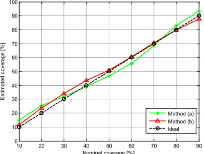
Figure 2.6 - Reliability diagrams of the proposed Bayesian methods. Estimated coverages (solid lines) are compared to the ideal coverages (dash line). ... 57

Figure 2.7 - Next-day forecasting. Estimated coverages of single predictors: Bayesian method, Markov chain method, and quantile regression method in November 2014. ... 69

Figure 2.8 - Next-day forecasting. Estimated coverages of the linear ensemble predictor and the probabilistic persistence method in November 2014. ... 69

Figure 2.9 - Next-day forecasting. PIT histograms of single predictors: Bayesian method, Markov chain method, and quantile regression method in November 2014. ... 70

Figure 2.10 - Next-day forecasting. PIT histograms of the linear ensemble predictor with MO and SO procedures, compared to the probabilistic persistence method in November 2014... 71

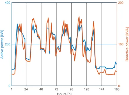
Figure 3.1 - Aggregate active and reactive powers from May 2, 2016 to May 8, 2016. ... 84

Figure 3.2 - Autocorrelation of the aggregate industrial active power ... 86

Figure 3.3 - Scatter plot of the aggregate industrial active power versus ambient temperature. ... 87

Figure 3.4 - Scatter plot of the aggregate industrial active power for each type of day, versus the hour of the day. The red lines indicate the mean values of observations. ... 88

Figure 3.5 - Scatter plots of the aggregate industrial active power in January, February, March, and April, versus the hour of the day. ... 89

Figure 3.6 - Scatter plots of the aggregate industrial active power in May, June, July, and August, versus the hour of the day. ... 90

vi

Figure 3.7 - Scatter plots of the aggregate industrial active power in September,

October, November, and December, versus the hour of the day. ... 90

Figure 3.8 - Scatter plots of the aggregate industrial active power for each

type of day versus the aggregate industrial active power measured one hour before. ... 92

Figure 3.9 - Scatter plots of the aggregate industrial active power for each

type of day versus the aggregate industrial active power measured one day before. ... 92

Figure 3.10 - Scatter plots of the aggregate industrial active power for each

type of day versus the aggregate industrial active power measured one week before. ... 93

Figure 3.11 - Normalized Mean Absolute Errors for the aggregate active power. .... 98

Figure 3.12 - Normalized Root Mean Squared Errors for the aggregate active

power: (a) comparison with benchmarks; (b) zoom on the models‘ errors ... 99

Figure 3.13 - Normalized Root Mean Squared Errors for the active power of the

electrical pump: (a) comparison with benchmarks; (b) zoom on the models‘ errors. ... 101

Figure 3.14 - Normalized Root Mean Squared Errors for the active power of the

carpentry feeder: (a) comparison with benchmarks; (b) zoom on the models‘ errors ... 102

Figure 3.15 - Normalized Root Mean Squared Errors for the active power of the

painting machine: (a) comparison with benchmarks; (b) zoom on the models‘ errors ... 103

Figure 3.16 - Normalized Root Mean Squared Errors for the aggregate reactive

power: (a) comparison with benchmarks; (b) zoom on the models‘ errors ... 105

Figure 4.1 - Gumbel fitting of dataset D2 through (a) MLE procedure; (b) ME

procedure; (c) QE procedure. ... 128

Figure 4.2 - Inverse Weibull fitting of dataset D2 through (a) MLE procedure;

(b) ME procedure; (c) QE procedure. ... 128

Figure 4.3 - Inverse Burr fitting of dataset D2 through (a) MLE procedure;

(b) ME procedure; (c) QE procedure. ... 129

Figure 4.4 - Generalized Extreme Value (a) and Gumbel (b) fitting of dataset

D13 through MLE procedure. ... 136

Figure 4.5 - Inverse Burr (a) and Inverse Weibull (b) fitting of dataset D13

through MLE procedure. ... 136

Figure 4.6 - Mixture Inverse Burr – Inverse Weibull fitting of dataset D13

through (a) MLE procedure, and (b) EM procedure. ... 137

Figure A.1 - Examples of reliability diagrams. ... 150

Figure A.2 - Examples of Probability Integral Transform histograms. ... 151

Figure A.3 - Graphical interpretation of the Continuous Ranked Probability

vii

List of tables

Table 1.1 - Utility of forecasting methods in power system operation needs ...8

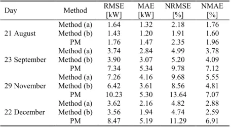
Table 2.1 - Spot-value error indices obtained through Bayesian method (a),

Bayesian method (b), and the persistence method for the

considered days ... 53

Table 2.2 - Spot-value error indices obtained through Bayesian method (a),

Bayesian method (b), and the persistence method for the considered test set ... 54

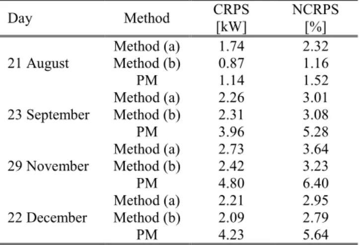
Table 2.3 - Probabilistic error indices obtained through Bayesian method (a),

Bayesian method (b), and the persistence method for the considered days. ... 55

Table 2.4 - Probabilistic error indices obtained through Bayesian method (a),

Bayesian method (b), and the persistence method for the considered test set. ... 56

Table 2.5 - Next-day forecasting. Values of weight coefficients for linear

ensemble in November 2014 ... 68

Table 2.6 - Next-day forecasting. Continuous ranked probability scores and

maximum deviation from perfect reliability in November 2014 ... 68

Table 2.7 - Next-day forecasting. Continuous ranked probability scores from

February to December 2014. ... 72

Table 2.8 - Next-day forecasting. Maximum deviation from perfect reliability

from February to December 2014. ... 72

Table 3.1 - Statistical parameters of the analysed load time series ... 85

Table 3.2 - Predictors candidate to build models for industrial load forecasts ... 95

Table 4.1 - Values of Gumbel, Inverse Weibull, and Inverse Burr parameters

estimated through MLE, ME, and QE procedures. ... 127

Table 4.2 - Kolmogorov-Smirnov test statistics and Chi-square test statistics for

Gumbel, Inverse Weibull, and Inverse Burr fitting distributions. Bold italic values denote failed tests, while underlined values correspond to the best-fitting distributions for each dataset. ... 130

Table 4.3 - Mean Absolute Errors in the Inverse Burr parameter estimation

procedures. ... 132

Table 4.4 - Mean Absolute percentage Errors in the Inverse Burr parameter

estimation procedures. ... 132

Table 4.5 - Values of Generalized Extreme Value, Gumbel, Inverse Weibull,

Inverse Burr, and mixture Inverse Burr – Inverse Weibull

parameters. ... 135

Table 4.6 - Chi-square test statistics and values of the Determination Coefficients

and Adjusted Determination Coefficients for datasets D3 and D7. Bold italic values denote failed tests, while underlined values

viii

Table 4.7 - Chi-square test statistics and values of the Determination Coefficients

and Adjusted Determination Coefficients for datasets D8 and D9. Bold italic values denote failed tests, while underlined values

correspond to the best-fitting distributions for each dataset. ... 138

Table 4.8 - Chi-square test statistics and values of the Determination Coefficients

and Adjusted Determination Coefficients for datasets D10 and D11. Bold italic values denote failed tests, while underlined values

correspond to the best-fitting distributions for each dataset. ... 138

Table 4.9 - Chi-square test statistics and values of the Determination Coefficients

and Adjusted Determination Coefficients for datasets D12 and D13. Bold italic values denote failed tests, while underlined values

correspond to the best-fitting distributions for each dataset. ... 139

Table 4.10 - Chi-square test statistics and values of the Determination Coefficients

and Adjusted Determination Coefficients for datasets D8 when random initial points are chosen. Bold italic values denote failed tests, while underlined values correspond to the best-fitting distributions for each dataset. ... 140

Table 4.11 - Results of the error analysis in terms of MAPEs, averaged for each

parameter of the mixture Inverse Burr – Inverse Weibull distribution estimated through the EM procedure, and for each value of the weight . ... 141

ix

List of abbreviations

ADC Adjusted Determination Coefficient

AMA Annual Maxima

ANN Artificial Neural Network

AR AutoRegressive

ARIMAX AutoRegressive Integrated Moving Average eXogenous

ARX AutoRegressive eXogenous

BI Bayesian Inference

BM Bayesian Method

CDF Cumulative Distribution Function

CRPS Continuous Ranked Probability Score

CS Chi-square

DC Determination Coefficient

D1,…,D13 Dataset 1,…,Dataset 13

EKF Extended Kalman Filter

ELM Extreme Learning Machine

EnKF Ensemble Kalman Filter

EM Expectation-Maximization

EWS Extreme values of wind speed

GARCH Generalized Autoregressive Conditional Heteroscedastic GEFCom Global Energy Forecasting Competition

GEV Generalized Extreme Value

GOF Goodness Of Fitting

GP Generalized Pareto

GU Gumbel

I Integrated

IB Inverse Burr

IW Inverse Weibull

KDE Kernel Density Estimation

KNN K-Nearest Neighbor

KS Kolmogorov-Smirnov

LFT Long Term Forecast

LPE Linear Pool Ensemble

MA Moving Average

MAE Mean Absolute Error

MAPE Mean Absolute Percentage Error

MC Markov Chain

MCMC Markov Chain Monte Carlo

ME Moment Estimation

MLE Maximum Likelihood Estimation

MLR Multiple Linear Regression

x

MO Multi-Objective

MTF Medium Term Forecast

M-IB-IW Mixture Inverse Burr - Inverse Weibull

NB Naïve Benchmark

NMAE Normalized Mean Absolute Error NRMSE Normalized Root Mean Square Error

NWP Numeric Weather Prediction

PDF Probability Density Function

PICP Prediction Interval Coverage Probability PINAW Prediction Interval Normalized Averaged Width

PIT Probability Integral Transform

PLF Pinball Loss Function

PM Persistence Method

PMA Period Maxima

POT Peak Over Threshold

PV Photovoltaic

QE Quantile Estimation

QM Quantile regression Method

QR Quantile Regression

QRF Quantile Random Forest

RG Renewable Generator

RMSE Root Mean Squared Error

RMSPE Root Mean Squared Percentage Error

SG Smart Grid

SN Seasonal naïve

SO Single Objective

STF Short Term Forecast

SVR Support Vector Regression

T1 model selection Technique 1

T2 model selection Technique 2

VSTF Very Short Term Forecast

WG Wind Generator

xi

List of symbols

ambient temperature at the forecast start time th _{bin of the probability space}

cloud cover at the forecast start time

unobservable data in the expectation-maximization algorithm

th _{unobservable value in the expectation-maximization algorithm}

white noise term at specific time

probability density function

probability density function of the Beta distribution used to model the hourly irradiance

probability density function of the Gamma distribution used to model the hourly clearness index

probability density function of the Generalized Extreme Value distribution

probability density function of the Gumbel distribution

probability density function of Inverse Burr distribution

probability density function of Inverse Weibull distribution

probability density function of the mixture Inverse Burr - Inverse Weibull distribution

̂ posterior predictive distribution of the hourly irradiance ̂ predictive posterior distribution of the hourly clearness index

forecast time horizon

_{smoothing parameter in kernel density estimation}

qualitative variable representative of the th _{hour of the day}

vector of qualitative variables representative of the hour of the day

counter

counter

forecast lead time

order of the moment of the probability density function _{parameter of the Tukey‘s test}

counter

number of inputs of a multiple linear regression model number of inputs of an artificial neural network number of inputs of support vector regression model number of inputs of k-nearest neighbors model number of inputs of quantile regression model number of inputs of lasso regression model ̅ median of the Gumbel distribution

̅ median of the Inverse Burr distribution ̅ median of the Inverse Weibull distribution

xii

consecutive states of the Markov chain

number of parameters of the considered probability distribution theoretical frequency of observations that lie in the th bin of the

probability space

pressure at the forecast start time

probability

un-normalized posterior distribution

̂ estimated probability

expected value of the log-likelihood of complete data in the expectation-maximization algorithm

ratio of the diffuse radiation in hours to the diffuse radiation in a day

residual white noise of the quantile regression model relative humidity at the forecast start time

counter

time

qualitative variable representative of the th _{type of day}

vector of qualitative variables representative of the type of day vector of weights of the linear pool ensemble

th _{weight of the linear pool ensemble}

th synaptic weight of artificial neural networks ̂ vector of estimated weights of the linear pool ensemble ̂ th estimated weight of the linear pool ensemble

vector of predictor variables

th _{predictor variable at generic time}

vector of predictor variables at generic time

vector of variables of interest

-quantile of the Gumbel distribution

-quantile of the Inverse Burr distribution

-quantile of the Inverse Weibull distribution ̂ forecast of the variable of interest at time

reference value for normalized error indices variable of interest at generic time

̂ forecast of the variable of interest at generic time

̂ estimated -quantile

̅ _{sample -quantile}

actual value of the variable of interest at time

complete data in the expectation-maximization algorithm

Markov chain transition matrix

fuzzy set

xiii

backward shift operator

Beta function

penalty coefficient of support vector regression hourly continuous ranked probability score test statistics of the chi-square test

expected value

cumulative distribution function

cumulative distribution function of the Generalized Extreme Value distribution

cumulative distribution function of the Gumbel distribution

cumulative distribution function of Inverse Burr distribution

cumulative distribution function of Inverse Weibull distribution

cumulative distribution function of the linear pool ensemble

cumulative distribution function of the mixture Inverse Burr - Inverse Weibull distribution

th _{cumulative distribution function combined in the linear pool}

ensemble

̂ estimated cumulative distribution function

hourly irradiance on a surfaced inclined by degrees

upper bound of the observed hourly irradiances on a surface inclined by degrees

Heaviside function

extra-terrestrial total solar radiation

total number of considered quantiles

diffuse fraction of total solar hourly radiation on a horizontal surface

hourly clearness index

upper bound of the observed hourly clearness indices

kernel function

test statistics of the Kolmogorov-Smirnov test Lagrange function in support vector regression log-likelihood of the Inverse Burr distribution

log-likelihood of the mixture Inverse Burr - Inverse Weibull distribution

likelihood of the mixture Inverse Burr - Inverse Weibull distribution

dimension of a time series

set of vectors of predictor variables of a regression model number of base predictors of the ensemble method

number of bins of the probability space

xiv

̅ _{mean value of observations that lie in each bin of the probability} space

number of states in Markov chain frameworks

subset of vectors of predictor variables of a regression model in k-nearest neighbors approaches

number of performed forecasts

dimension of the training set of a Bayesian model

dimension of the training set of an exponential smoothing model

dimension of the training set of the Bayesian model for the hourly solar irradiance

dimension of the set to evaluate the goodness of fitting of distribution

dimension of the training set to estimate parameters of the Inverse Burr distribution

_{dimension of the training set of the Bayesian model for the hourly} clearness index

dimension of the training set of a kernel density estimation model

dimension of the training set of a k-nearest neighbors model

dimension of the training set of a lasso egression model

dimension of the training set of a multiple linear regression model

dimension of the training set to estimate parameters of the mixture Inverse Burr - Inverse Weibull distribution

dimension of the training set of a naïve benchmark model

dimension of the training set of a Nielsen model

dimension of the training set of a probabilistic extension of the persistence approach

_{dimension of the training set of the quantile regression method}

dimension of the training set of a support vector regression model

Gaussian distribution

active power at time

contribution to the pinball loss function of the -quantile at time photovoltaic power at the time horizon

rated power of the photovoltaic generator

-quantile of photovoltaic power

actual value of photovoltaic power

̂ estimated active power at time

̂

estimated -quantile of the linear pool ensemble of photovoltaic power

xv

̂ persistence active power forecast ̂ seasonal naïve active power forecast

ratio of the beam radiation on a tilted surface to the beam radiation on a horizontal surface

adjusted determination coefficient determination coefficient

surface area of the photovoltaic array

th _{state in which the variable of interest lies at specific time}

vector of ambient temperatures vector of cloud cover

vector of hourly solar irradiances

vector of hourly clearness indices

vector of pressures

vector of relative humidity

seasonal period

universe of discourse

quantile level

_{smoothing coefficient of exponential smoothing models}

coefficient of Nielsen

̂ estimated quantile level

̂ estimated quantile level of the linear pool ensemble degrees of inclination of photovoltaic modules

th _{parameter of the hourly solar irradiance regression model}

th _{parameter of the hourly clearness index regression model}

th parameter of a lasso regression model

th parameter of a multiple linear regression model th _{parameter of a support vector regression model}

̂ estimated sample of the th _{parameter of the hourly solar irradiance}

regression model

̂ estimated sample of the th _{parameter of the hourly clearness index}

regression model

̂ th estimated parameter of a lasso regression model

̂ th _{estimated parameter of a multiple linear regression model}

̂ th _{estimated parameter of a support vector regression model}

_{vector of parameters of the lasso regression model}

_{vector of parameters of the multiple linear regression model vector of parameters of the support vector regression model vector of parameters of the quantile regression model}

xvi

̂ _{vector of estimated parameters of the lasso regression model} ̂ _{vector of estimated parameters of the multiple linear regression}

model

̂ _{vector of estimated parameters of the support vector regression} model

̂ _{vector of estimated parameters of the quantile regression model} shape parameter of the Inverse Burr distribution

̅ Euler-Mascheroni constant

parameter of the modified Gamma distribution shape parameter of the Inverse Weibull distribution error band of the support vector regression

error term of a multiple linear regression model shape parameter of the Inverse Burr distribution

th _{Lagrange variable in support vector regression} th _{Lagrange variable in support vector regression}

global efficiency of the photovoltaic array

moving average operator

vector of parameters in Bayesian frameworks

scale parameter of the Generalized Extreme Value distribution shape parameter of the Generalized Extreme Value distribution

parameter of the modified Gamma distribution

vector of Lagrange variables in support vector regression th _{Lagrange variable in support vector regression}

_{degree of regularization of lasso regression}

vector of Lagrange variables in support vector regression th _{Lagrange variable in support vector regression}

̂ vector of estimated Lagrange variables

̂ vector of estimated Lagrange variables

mean value of the Beta distribution

mean value of the modified Gamma distribution

mean value of the Generalized Extreme Value distribution mean value of the Gumbel distribution

mean value of the Inverse Burr distribution mean value of the Inverse Weibull distribution

mean value of the mixture Inverse Burr - Inverse Weibull distribution

mean value of the last measured observed hourly solar irradiances

mean value of the last measured observed hourly clearness indices

xvii

̂ estimated mean value of the Beta distribution

̂ estimated mean value of the modified Gamma distribution scale parameter of the Inverse Weibull distribution

augmentation coefficient of support vector regression at generic time

augmentation coefficient of support vector regression at generic time

vector of augmentation coefficients of support vector regression vector of augmentation coefficients of support vector regression

first weight of the multi-objective optimization problem

second weight of the multi-objective optimization problem ̂ vector of estimated augmentation coefficients of support vector

regression

̂ vector of estimated augmentation coefficients of support vector regression

shape parameter of the Gumbel distribution

_{probability of the variable of interest to lie in the} th _{state at time}

vector of state probabilities of the variable of interest at time scale parameter of the Inverse Burr distribution

error term of the probabilistic persistence approach shape parameter of the Beta distribution

̂ estimated sample of the shape parameter of the Beta distribution variance of the Generalized Extreme Value distribution

variance of the Gumbel distribution variance of the Inverse Burr distribution variance of the Inverse Weibull distribution

variance of the mixture Inverse Burr - Inverse Weibull distribution

standard deviation of the probabilistic persistence approach ̅ _{threshold of artificial neural networks}

̅ _{threshold of the expectation-maximization algorithm} ̅ _{threshold of support vector regression}

location parameter of the Generalized Extreme Value distribution shape parameter of the Beta distribution

location parameter of the Gumbel distribution

maximum value of absolute deviations between estimated and actual coverages

weight parameter of the mixture Inverse Burr - Inverse Weibull distribution

̂ expectation-maximization estimation of the weight of the mixture Inverse Burr - Inverse Weibull distribution

xviii

parameters estimated in the expectation-maximization algorithm ̂ _{initial set of parameters of the expectation-maximization algorithm} ̂ _{binary indicator of a generic estimated -quantile}

̂

binary indicator of the estimated -quantile of the linear pool ensemble

first objective function to be minimized in the multi-objective ensemble method, i.e., the average value of hourly continuous ranked probability scores

second objective function to be minimized in the multi-objective ensemble method, i.e., the maximum value of all absolute deviations between estimated and actual coverages

stationary AR operator

input operator

xix

Acknowledgment

After these three years, I recognize that pursuing a Ph.D. was the best choice I ever made in my entire life. But when you reach such a great achievement, enjoying every moment of it, the least you can do is to express your gratitude to everyone made it possible.

My tutor, prof. Guido Carpinelli, is more than an academic advisor. His dedication to research and teaching is exemplary, and his competence and passion towards every field of application in electrical engineering is an incitement for everyone is so blessed to work with him. His attitude of respect towards collaborators, professors, researchers, and students, should be a reference point for everybody who aims to pursue an academic career.

My co-tutor, dr. Antonio Bracale, is a role model in terms of proficiency and enthusiasm towards the academic research. His theoretical and technical skills are extraordinary and he dedicated himself to improve my skills too, through his daily support in my Ph.D. activities.

Although not officially, prof. Pierluigi Caramia was essentially my third tutor. I don‘t remember a single circumstance in which he was not able to support or help me. His positive and constructive attitude towards me was an added value during these years.

Guido, Antonio, and Pierluigi made me feel a member of the team, a member of the family.

I thank my coordinator, prof. Daniele Riccio; he played his institutional role with an uncommon willingness towards me and my colleagues, always understanding our needs. I am also grateful to prof. Mario Russo, prof. Filippo Spertino, and prof. Paola Verde, for critically reviewing my Ph.D. thesis. Their useful suggestions and advices allowed me to significantly improve my dissertation.

I have sincerely appreciated the opportunity to work with several excellent academic researchers during my Ph.D. course. I thank dr. Tao Hong, dr. Andrea Michiorri, and prof. Renato Rizzo for their priceless contributions in developing my skills and in my personal growth. I have really enjoyed working with prof. Mario Pagano and prof. Angela Russo; their expertise exactly matches their kindness.

xx

Prof. Elio Chiodo deserves a special mention: he acts not only as a scientific partner, but also as a friend.

My daily experience would not have been so complete without prof. Amedeo Andreotti, prof. Davide Lauria, prof. Daniela Proto, and prof. Pietro Varilone; they are people of absolute value, and outstanding professors. I established a genuine friendship with dr. Luigi Pio Di Noia and dr. Fabio Mottola: two nice guys who share an extraordinary research versatility.

I could have not fully dedicate myself in pursuing my Ph.D. without the unconditional support of my parents, Marisa and Vincenzo. I hope to reward them with my love and with my accomplishments. I want to express my gratitude also to my ―brothers‖ Ivan and Carmine, for the time spent together as ka-tet.

My greatest ―thank you‖ definitely goes to Luisa, my font of happiness during these years and forevermore (and a bit more). She is the one who helps me, teaches me, questions me, loves me, but most importantly she gives new meanings to my life every day.

1

I

NTRODUCTION

In the new liberalized markets a multitude of operators is allowed to interact with transmission and distribution networks, both by purchasing or selling energy. In this context, renewable generators supply a significant share of the total electricity demand, saving

thousands of tons of CO2 and polluting agents from being released in

the atmosphere each day. The old paradigm of static networks is going to be surpassed by intelligent structures, with a widespread diffusion of distributed generation, information technologies, and control devices that foster the optimal exploitation of energy resources.

These are great achievements in pursuing social wellness and technology advance, with care to the environment. However, the path to smarter electrical grids is very intricate, and many complications that were unimaginable two decades ago are now part of the daily routine of transmission and distribution grid managers.

One of the biggest problem is facing with forecasting.

Until ‗90s, the main topic of forecasting was, by far, the load consumption at aggregate national, regional or sub-station levels. Load forecasts were required for short-term and long-term scenarios, in order to respectively i) assure power balancing and ii) plan future expansions of the networks in decennial schedules.

Nowadays, many other variables (i.e., renewable generation powers, extreme values of weather variables, loads at disaggregate levels, and energy prices) are the subject of forecasting.

The spread of renewable generators has, in fact, extended the problem of forecasting also to the generation powers and extreme values of weather variables, such as wind speeds.

Renewable generation power forecasting, with particular focus on wind and photovoltaic (PV) systems, is yet to be fully explored in relevant literature. Indeed, forecasting systems found in literature for these variables are deterministic tools in the majority of cases: they

2

only provide a spot-value as forecast. The need of probabilistic tools, that are able to catch also information on the uncertainty linked to the wind and solar energy sources, has only recently been recognized by electrical practitioners, and researches in this framework are well encouraged since 2010s.

Extreme values of wind speed (EWS) play a key role in wind power forecasting, in the overhead line rating, and in the assessment of the mechanical reliability of system components; in such kinds of applications, risk analyses are encouraged and probabilistic tools are needed. An accurate statistical characterization of such events is mandatory to improve the quality of several EWS probabilistic forecasting tools, since they usually require the definition of an appropriate Probability Density Function (PDF) to perform with high accuracy.

Another new forecasting issue is the need of forecasts for loads at disaggregate levels, and of forecasts of both active and reactive powers. It is fostered by the growing ability of new management and regulation tools to push the optimal exploitation of energy sources in smart power systems. Having active and reactive power profiles available in advance is mandatory in order to perform the correct scheduling to manage grids at consumers level (e.g., micro-grids). Eventually, also energy price forecasts are currently required for the convenient participation of operators to electric markets.

In summary, forecasting in power systems is a wide topic that today covers many and many needs, and that requires further research efforts.

In this wide and complex context, after a brief discussion on the classification of forecasting systems and on the methods that are currently available in literature for forecasting electrical variables, stressing pros and cons of each approach, the thesis provides four contributions to the state of the art on forecasting in power systems where literature is somehow weak.

The first contribution is a Bayesian-based probabilistic method to

forecast PV power in short-term scenarios. The method transforms probabilistic forecasts of the hourly solar irradiance (or the hourly clearness index) into probabilistic forecasts of the PV power by means of well-known relationships, in an indirect approach. Solar irradiance

3

(or hourly clearness index) is modeled by means of an analytic PDF, whose parameters are estimated by means of the Bayesian inference of past available observations. An exogenous linear regression model is also defined in order to link one of the PDF parameters to the measurements of some influencing weather variables.

The second contribution is a probabilistic competitive ensemble

method once again to forecast PV power in short-term scenarios. The

idea is to improve the quality of forecasts obtained by means of some individual probabilistic predictors, by combining them in a probabilistic competitive approach. Since the probabilistic predictors may vary in terms of predictive outputs (e.g., they can provide predictive samples, predictive PDFs, or predictive quantiles), in the proposed ensemble method the forecasts obtained through base predictors are firstly properly combined through a linear pooling of predictive cumulative density functions. Then, in order to guarantee elevate sharpness and reliability characteristics, a multi-objective (MO) optimization method is proposed and applied during the training period in order to estimate coefficients of the linear pooling. The MO optimization is specifically devoted to overcome well-known problems resulting in the over-dispersion of forecasts coming from the probabilistic combination of probabilistic base predictors in the linear pool approach. The Bayesian method (i.e., the first proposed contribution), a Markov chain method, and a quantile regression method are selected as probabilistic base predictors to be merged.

The third contribution is aimed to the development of a deterministic

industrial load forecasting method suitable in short-term scenarios, at

both aggregated and single-load levels, and for both active and reactive

powers. The deterministic industrial load forecasting method is based

on Multiple Linear Regression (MLR) or Support Vector Regression (SVR) models. The selection of most adequate models is performed with two different techniques. The first technique is based on the 10-fold cross-validation of multiple MLR and SVR models that contain combinations of the informative inputs; the best MLR and the best SVR models (in terms of average errors) are selected for the test step. The second technique is instead based on the lasso analysis, in order to directly draw the most useful inputs among the informative ones; a

10-4

fold cross-validation is performed also in this case, in order to provide coherent comparison with the first technique.

The fourth contribution provides advanced PDFs for the statistical characterization of EWS.

In particular, one of the PDFs proposed in this Thesis is an Inverse

Burr distribution for EWS modeling. The derivation process of the

Inverse Burr distribution is discussed, and a rigorous parameter estimation procedure based on the quantile estimation is provided and compared to classical maximum likelihood estimation and moment estimation procedures. In some conditions, the quantile estimation procedure consists in solving an analytic equation, thus avoiding the well-known convergence problems of classical estimation procedures.

The other PDF proposed in this Thesis is a mixture Inverse Burr –

Inverse Weibull distribution for EWS modeling. The mixture of an

Inverse Burr and an Inverse Weibull distribution allows to increase the versatility of the tool, although increasing the number of parameters to be estimated. This complicates the parameter estimation process, since traditional techniques such as the maximum likelihood estimation suffer from convergence problems. Therefore, an Expectation-Maximization (EM) procedure is specifically developed for the parameter estimation. The aim of the EM procedure is still to maximize the likelihood of an observed EWS dataset, although hypothesizing additional, hidden parameters to simplify the formulation of the likelihood function.

This thesis is organized in four Chapters and an Appendix.

The first Chapter provides an overview of the classification of forecasting methods in power systems based on the needs of electrical operators, and a brief explanation of the main methods available in relevant literature.

The second Chapter explores in details the state of the art on probabilistic PV power forecasting, and shows the two contributions of this thesis in that field.

The state of the art on industrial load forecasting is presented in details

in the third Chapter; the related contribution (i.e., the deterministic

5

The fourth Chapter deals with EWS modelling; after discussions on the state of the art, the two proposed models and their corresponding parameter estimation procedures are presented.

Numerical applications related to each of the proposed contributions are shown in the ending parts of second, third and fourth Chapters; actual data are used in all of the numerical applications, in order to effectively test the validity of the proposals in real-world scenarios. Eventually, the main error indices and tools for the assessment of forecasts in both deterministic and probabilistic frameworks, and for the assessment of the Goodness Of Fitting (GOF) distributions, are shown in the Appendix.

6

Chapter 1.

F

ORECASTING AND POWER SYSTEMS

1.1.

I

The planning, operation and management of power systems are strongly affected by weather conditions, social factors, and economic factors [1-5].

Solar irradiance, wind speed and ambient temperature, in fact, are weather conditions that strongly affect the production of PV and wind (WGs) generators, and the ampacity of overhead lines [6,7]. EWS may seriously damage electrical installations such as wind towers, WG blades, overhead lines and trellis [3,8-10]. Ambient temperature also influences energy demand due to the spread of cooling and heating systems [11,12], and transformer loadability due the variations in thermal exchange [13].

Social and economic factors modify the human attitude toward energy consumption, as wealthier societies tend to consume more energy, and they also affect the supply from renewable sources, as more generators are typically installed in periods of high incentives [5,14]. Price variations on energy markets play a key role in the optimal management of transmission and distribution systems [15,16].

The increasing complexity of electrical networks makes the whole power system more vulnerable to the abovementioned factors and, then, power system operators would appreciate to perfectly prior know the future status of the grids, in order to plan and perform their actions with no miscalculations or approximations [17]. However, this is not feasible.

The above problems, in addition, will definitely grow in interest in next years due to the continuous development of Smart Grids (SGs) and Micro Grids (μGs): adequate criteria of management and planning of transmission and distribution networks should be developed in these

7

new frameworks, thus requiring more accurate and reliable forecasting methods to be applied in power systems. In particular, forecasting non-controllable generation, loads and market prices is therefore mandatory in order to help the future decision-makers to optimally exploit energy sources, assuring the balance and stability on networks, and favoring the risk assessment in reliability and maintenance tasks [18-20].

The forecasting methods applied in power systems are briefly summarized in this Chapter. First, their typical classifications are provided in Section 1.2. Then, forecasting approaches that have been widely applied in relevant literature to power systems are discussed in Section 1.3.

1.2.

C

The diversity in forecasting needs has a direct, intuitive consequence: no forecasting method is universally able to fit any purpose, but it has to be selected case by case on the basis of particular needs [21]. The classifications of forecasting methods straightforwardly follows the diversity in terms of end user needs.

The first classification is made in terms of forecast lead time. Indeed, actions on power systems are performed on different time lines: e.g., improvement, replacement or realization of new infrastructures are planned several years before, while optimal management of distributed energy resources in SGs and μGs is scheduled some minutes to some hours before [1,22].

Few papers [23] classify forecasting methods in 2 categories (short-term and long-(short-term); however, the most complete practice is to

individuate Very Short-Term Forecasting (VSTF), Short-Term

Forecasting (STF), Medium-Term Forecasting (MTF), and Long-Term

Forecasting (LTF) methods [24-28].

VSTF lead times range up to 24 hours1; they are usually involved in

power balancing and system optimal management and control. The influence of external variables (e.g., ambient temperature for load

1 _{There is a lack of standardized classification. Therefore, some papers refer to}

VSTF when lead times are up to 30 minutes; in this case, STF lead times range from 30 minutes to 24-48 hours ahead.

8

forecasting) is limited in this kind of applications, and therefore is often overlooked.

STF lead times range from 24 hours ahead to two weeks ahead; they are usually involved in power balancing for acquiring appropriate reserve, market participation, and system optimal management.

MTF lead times range from 2 weeks to 3 year ahead; this wide interval of time makes MTF methods useful for market participation, system optimal management, and planning. Social and economic factors should be carefully investigated in MTF, especially for monthly and yearly scenarios.

LTF lead times start from 3 years and reach 20 (or more) years. These forecasts are involved in power system planning, and weather, social and economic long-term evaluations are mandatory in order to cope with evolutionary trends.

Table 1.1 associates forecasting methods, classified in terms of lead times, to corresponding needs [28].

Table 1.1 - Utility of forecasting methods in power system operation needs

Classification of forecasting methods

Power system operation need Power balancing Participation to electrical markets Optimal management and control Planning VSTF yes no yes no

STF yes yes yes no

MTF no yes yes yes

LTF no no no yes

A second classification involves the output of forecasting methods. This comes from the different risks linked to power system tasks that require forecasts to be completed.

Let‘s think of a wind plant owner, who wants to sell energy on electrical markets [29]. He has to submit a selling offer, stating the (exact) amount of energy he will be able to produce; in several Countries, he is penalized if the resulting production is too far from the declared one. If he disposes of a forecasting method that provides only a single value of wind power as output, the plant owner has no other choice than submitting a selling offer of as much energy as the forecasted one. Instead, if he disposes of a forecasting tool that

9

provides more values, or the probability distribution of wind powers, he can manage the forecasts and make the best choice for his needs.

In this context, deterministic forecasts provide as output only a single

value of the variable of interest (point forecast). Probabilistic forecasts

provide as output analytical distributions such as PDFs, Cumulative Density Functions (CDFs), sampled distributions (discrete

probabilities), quantiles2, or moments of the predictive distribution

(e.g., mean, variance and skewness) [30]. Note that the variable of interest is still treated as a random entity in both frameworks: the main difference is that a single value is given as forecast of the variable of interest in deterministic framework, while more values, or a function, are given as forecast of the variable of interest in probabilistic framework.

Probabilistic forecasts are generally preferable, since they provide also information about the uncertainty linked to the forecast itself. Therefore, they allow the risk assessment and the optimal selection of a single value, on the basis of different frameworks [31,32]. Indeed, it is always possible to extract a single, spot-value (e.g., the mean value of the predictive distribution) from probabilistic forecasts, while the reciprocal is obviously not valid. The main drawbacks of probabilistic forecasts are the increase of method complexity, and their greater computational burden. Then, if the forecast end user gains no benefit in having a probabilistic forecast, deterministic methods are still the best choice.

It is worth noting that probabilistic methods sometimes rely on an underlying deterministic method [33,34]; e.g., some parameters of the predictive probabilistic distribution could be set from the output value of a deterministic method. In this case, improving the performance of the underlying deterministic method is compulsory in order to increase the overall quality of the probabilistic forecasts. Thus, research efforts in the deterministic framework are always encouraged.

A third classification of forecasting methods is based on the characteristics of models involved in the forecasting method, and

2 _{Let‘s recall that the -quantile of a probability distribution is the value of the}

10

consequently on the solving procedure. The common classification is

in terms of parametric and non-parametric methods.

Parametric methods are based on models that are univocally identified as several numerical parameters are known; e.g., a predictive analytical Gaussian distribution is univocally identified when its mean and variance are known. Therefore, solving a parametric forecasting method consists in finding estimations of unknown parameters, usually by minimizing or maximizing assigned objective functions (i.e., by minimizing an error index). In the particular case of parametric probabilistic methods, usually the problem of finding a prior probabilistic characterization of the variable of interest through a specific PDF has to be solved [33].

Non-parametric methods, instead, rely on the idea that forecasting future dynamics can be achieved by analogy with past dynamics. Indeed, the variable under study is not assessed through an analytic model, instead it is forecasted by means of a procedure that ―learns‖ from the past. Note that the ―non-parametric‖ definition could be misleading. It does not mean that no parameters are involved in non-parametric methods; indeed, some involved parameters could identify the order of the model, rather than the model itself.

In non-parametric methods, however, the complexity of the models (i.e., the number of parameters) grows with the dimension of the problem and, theoretically, is not constrained. The more the inputs (i.e., the elements of the training set) fed to the non-parametric method, the larger is the number of parameters to be estimated. Therefore, the structure of the model itself ―grows‖ as the training set enlarges (Fig. 1.1). On the other hand, the structure of models in parametric methods is fixed with the dimension of the problem; the same number of parameters has to be estimated, regardless of the size of the training

set3 (Fig. 1.1).

3 _{Training set stores all of the available input data used to estimate model}

parameters. Since the actual values of the variable of interest are known, forecasts are produced in-sample during the training period. A test period is therefore necessary to fairly evaluate the performance of the so-built forecasting model, in an out-of-sample context.

11

Figure 1.1 – Features of parametric and non-parametric methods.

The fourth and last classification is based on the approach used to

build and solve the forecasting problem. Statistical approaches rely on

measurement data acquired in the past to produce forecasts for the future, starting from the assumption that past conditions are

informative for the future. Physical approaches rely instead on a

specific formulation of the problem under study in a rigorous fashion, by exploiting mathematical formulas based on physical principles.

Hybrid approaches can be a combination of statistical approaches,

physical approaches, or statistical and physical approaches together.

1.3.

F

A review of common forecasting methods applied to power systems is presented in this Section. The latter classification of Section 1.2, i.e., statistical approaches, physical approaches, and hybrid approaches, is considered in the following. The main features of each approach are briefly discussed in the corresponding sub-Sections.

12

1.3.1. Statistical approaches

Statistical approaches exploit information provided by the observed past history to describe and forecast the realization of a physical phenomenon.

In several kinds of applications, a mathematical model is formulated to characterize the variable of interest. If the past were able to exactly describe its behavior (e.g., if the mathematical model can be formulated from well-known physical laws), the model would be purely deterministic, and forecasting future values of the variables simply consists in solving an equation from assigned input data. However, in the majority of cases, there are many random events that could affect the realization of the phenomenon, and, therefore, models can deviate from classical physical laws, since they could fail to exactly predict the future conditions. Thus, models can be built on the basis of previous experiences in order to take into account the effect of external random events on the objective variable.

In other applications, no strict mathematical model is needed in order to forecast the future values of the variable of interest. This is the case, of machine learning approaches, as the artificial intelligence of computers ―learns‖ from the past and tries to find the underlying relationships between inputs and outputs. Due their versatility, machine learning approaches are suitable for both deterministic or probabilistic forecasting.

1.3.1.1. Naïve approaches

Naïve approaches are techniques that allow to produce forecasts that can surprisingly be accurate in VSTF and STF frameworks, despite their superior simplicity. For this reason, they are usually adopted as benchmarks, to give a comparative reference for assessing the quality of forecasts coming from more complex models.

The first notable naïve approach is based on the persistence of the

variable of interest. In other words, the variable of interest is

expected not to vary during the forecast lead time , thus assuming the

forecast ̂ at the time horizon the same value experienced at the

forecast start time :

13

Note that, to take into account the eventual seasonal behavior of the variable of interest, a seasonal naïve (SN) benchmark, direct extension of the persistence approach, can be expressed as follows:

̂ , (1.2)

where is the seasonal period (e.g., daily or weekly).

Both the abovementioned naïve benchmarks use only one past measured value of the variable. This could result in an over-sensitive approach, since it directly depends on a single value that could lose generality. The average naïve benchmark (NB) overcomes this

problem by providing a forecast as an average of past measured

values of the variable of interest, as follows: ̂ ∑ . (1.3)

Obviously, the average naïve benchmark could suffer from a dual problem: it could over-generalize the behavior of the variable of interest, losing valuable information linked to recency.

An interesting compromise between the persistence and the average naïve models was proposed by Nielsen et al. in [35]. In the Nielsen

approach, the forecast ̂ is obtained as a weighted sum of the last

_{available observation and of the average of past observations:}

̂ ∑ , (1.4)

where the Nielsen weight coefficient is a function of the lead

time , and it is analytically computed from the correlation between

lagged observations as:

∑ ̃ ̃ ∑ ̃ , (1.5)

14 where ̃ ∑ .

As said before, naïve benchmarks are often used as deterministic benchmarks due their intuitiveness and simplicity. Extensions of all of these naïve approaches to probabilistic frameworks exist, and have been extensively applied in relevant literature to build also probabilistic benchmarks.

In the probabilistic persistence approach, e.g., it is common to

introduce a probabilistic error term from a Gaussian

distribution with zero mean, and standard deviation equal to

the variance of past errors:

√ ∑ ̂ . (1.6)

Thus, from the probabilistic model:

̂ , (1.7)

it is possible to extract predictive samples or to evaluate predictive quantiles of the variable of interest. Note that also the predictive PDF could be built in an analogous way, e.g., assuming is a Gaussian

distribution with mean and standard deviation .

The same approach could be adapted also to other distribution families, mirroring the prior assumption on the distribution family in the model that is to be compared with the naïve benchmarks. The assumption on the distribution family is, therefore, a key point.

Naïve approaches have been extensively applied in literature relevant to power systems, mostly as deterministic and probabilistic reference methods; relevant papers are recalled in surveys on load forecasting [6,24,28,36-44], PV forecasting [27,36,45-54], WG forecasting [30,47,48,55-64], and price forecasting [15,65-67].

15

1.3.1.2. Regression analysis

Regression analysis is a technique that allows to find and to model the intrinsic relationships between the variable of interest (i.e., the dependent variable) and one or more other variables (i.e., the

independent variables4) [68,69].

The most common approach in regression analysis is to model the conditional expectance of probability distribution of the variable of interest, assuming that the variance does not changes with varying conditions. However, in many application the focus is transferred to modeling some quantiles of the probability distribution of the variable of interest (Quantile Regression, QR), or some other specific parameters of the underlying probability distribution. In all of these cases, however, the target is a mathematical function (regression function) of the independent variables.

Regression analysis can be both parametric and non-parametric. In the first case, unknown parameters have to be estimated in order to univocally determine the regression function. In the second case, specific techniques can be used to identify the model in an infinite-dimensional space of functions.

The simplest, parametric regression approach is the linear regression.

The dependence between the dependent variable and independent variable(s) is linear in the parameters, meaning that parameters are only coefficients to independent variables. If two or more independent variables are considered, it is common to refer to MLR approaches. The general form of a MLR model is:

̂ , (1.8)

where ̂ is the forecast at time , are the predictors,

are the unknown parameters of the

model, and is a white noise term.

MLR models are fitted to data available in the training set trough least square approach (i.e., by minimizing the sum of squared errors in the

4 _{Dependent variables are also denoted in relevant literature as response variables}

or regressand. Independent variables are also denoted in relevant literature as explanatory variables, predictors, or regressors.

16

training set), although several approaches (such as lasso estimation [70]) provide some accurate results in many kind of situations by minimizing the lack of fit through different norms.

Further regression approaches are nonlinear in the parameters [69]. The model development can be performed on the basis of prior experience. It is important to note that nonlinear models are not so uncommon as one may think; e.g., if the response variable is assumed to be always positive, the constraint often leads to a nonlinear model. Obviously, estimating the parameters in this function is more challenging than estimating parameters in linear models. If nonlinear models can be brought to linear models through specific transformations, they are usually referred as intrinsically linear models. A well-known example is the following regression model:

̂

, (1.9)

that can be easily linearized through the logarithmic transformation [69], resulting in:

̂ ̂ . (1.10) Regression approaches have been extensively applied in literature relevant to power systems, in both deterministic and probabilistic fashion; relevant papers are recalled in surveys on load forecasting [6,24,28,36-44], PV forecasting [27,36,45-54], WG forecasting [30,47,48,55-64], and price forecasting [15,65-67].

1.3.1.3. Univariate stochastic time series

A time series is a set of sequential observations of the

variable of interest; the dependency on time is here implicit, as

subscripts stand for . When the time

series is the sample manifestation of a stochastic process, it is denoted as univariate stochastic time series [71,72].

The main characteristic in time series analysis is the dependency between ―adjacent‖ observations; the exploitation (and coherent modeling) of such dependency is of practical use in building a model

17

that is representative of the stochastic process, starting from the available time series.

Models used to capture the features of a time series fall into the AutoRegressive (AR), Moving Average (MA), and