“© 2016 IEEE. Personal use of this material is permitted. Permission from IEEE must be
obtained for all other uses, in any current or future media, including reprinting/republishing this
material for advertising or promotional purposes, creating new collective works, for resale or
redistribution to servers or lists, or reuse of any copyrighted component of this work in other
works.”
Place Classification with a Graph Regularized Deep Neural Network
Yiyi Liao,
Student Member, IEEE,
Sarath Kodagoda,
Member, IEEE,
Yue Wang, Lei Shi,
Member, IEEE,
and Yong Liu,
Member, IEEE
Abstract—Place classification is a fundamental ability that a robot should possess to carry out effective human-robot interactions. In recent years, there is a high exploitation of Artificial Intelligence algorithms in robotics applications. In-spired by the recent successes of deep learning methods, we propose an end-to-end learning approach for the place clas-sification problem. With deep architectures, this methodology automatically discovers features and contributes in general to higher classification accuracies. The pipeline of our approach is composed of three parts. Firstly, we construct multiple layers of laser range data to represent the environment information in different levels of granularity. Secondly, each layer of data is fed into a deep neural network for classification, where a graph regularization is imposed to the deep architecture for keeping local consistency between adjacent samples. Finally, the predicted labels obtained from all layers are fused based on confidence trees to maximize the overall confidence. Experimental results validate the effectiveness of our end-to-end place classification framework in which both the multi-layer structure and the graph regularization promote the classification performance. Furthermore, results show that the features automatically learned from the raw input range data can achieve competitive results to the features constructed based on statistical and geometrical information.
Index Terms—Place classification, graph regularization, deep learning
I. INTRODUCTION
P
LACE classification is an important problem in human-robot interactions and mobile human-robotics, which aims to distinguish differences of environmental locations and assign a label (corridor, office, kitchen, etc.) to each location [1], [2]. It allows robots to achieve spatial awareness through semantic understanding rather than having to rely on precise coordinates in communicating with humans. Furthermore, the semantic labels has the potential to efficiently facilitate other robotic functions such as mapping [3], behavior-based navigation [4], task planning [5], [6] and active object search and rescue [7]. Therefore, the task of place classification has been intensively explored in the robotics community [8], [9], [10].In general, place classification is carried out through en-vironment sensing. Laser range finders, cameras and RGB-D sensors are the mostly used sensing modalities. Location and topological information can also be informative in place classification. In this work, we attempt to exploit both the sensory data and location information. We assume all the maps in this paper contain these two parts of information and some
Yiyi Liao, Yue Wang and Yong Liu are with the State Key Laboratory of Industrial Control Technology and Institute of Cyber-Systems and Control, Zhejiang University, Zhejiang, 310027, China (Yong Liu is the corresponding author of this paper, e-mail:[email protected]).
Sarath Kodagoda and Lei Shi are with the Centre for Autonomous Systems (CAS), The University of Technology, Sydney, Australia.
of the maps are labeled with human knowledge. Then the place classification problem can be stated as predicting the labels of new environments given the labeled maps.
By analysing those two forms of data, sensory data and location information, we can gain insights into the char-acteristics of the place classification problem. Raw sensory data encode the environment information at different loca-tions which can provide discriminative information between different classes. However, this requires an effective feature extraction method and most of the previous works tend to extract hand-engineered features from the raw data [11], [12]. Our opinion is that the handcrafted features may not fully exploit the potential to achieve higher generalization ability. On the other hand, locations encode spatial information of the environment and indicate local consistency of the labels, which means the positions at spatial proximity have higher probability of having the same class labels.
It is to be noted that another difficulty in place classification is the influence of different field of views (FOV) of the sensors used. For example, the data collected by a 180◦ FOV laser range finder facing approximately a corner of a corridor may not contain sufficient information for classification. If the laser range finder collects 360◦ FOV data at a door of an office room, the robot might be confused by mixed information from two classes.
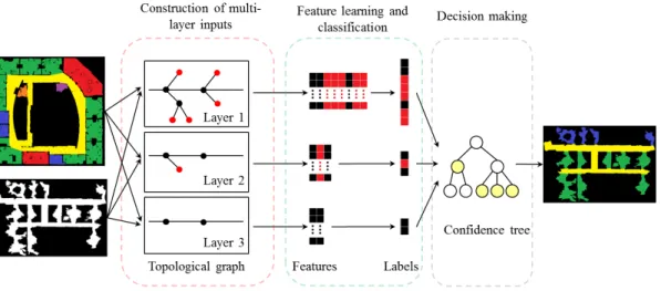
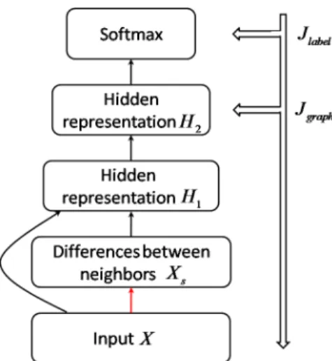
In order to address these problems, in this paper, we propose a graph regularized deep learning approach with classification on multi-layer inputs. The pipeline of our system is illustrated in Fig. 1, which can be split into three parts:
1) Construction of multi-layer inputs: The environmental information is represented through the generalized Voronoi graph (GVG) [13], a topological graph in which the nodes correspond to the sensory data and the edges denote the relationships in this paper. By fusing the information and eliminating the end-nodes, we implement a recursive algorithm to construct multi-layer inputs with hierarchical GVGs. The inputs of higher layers contain information of larger field of view, represented by increasingly succinct GVG. The features are extracted from each layer of input and classified indepen-dently.
2) The graph regularized deep architecture for feature learning and classification: We adopt the deep architecture that learns features from the raw data automatically. A graph regularizer is imposed to the deep architecture to keep the local consistency, where an adjacency graph is constructed to depict the adjacency and similarity between the samples. Our training map and testing maps are fed into the deep architecture for feature learning at the same time, which forms a semi-supervised learning framework. The output of this step is the predicted labels of different layers.
Fig. 1. Pipeline of the semi-supervised learning system. Given a training map and a testing map, firstly multi-layer inputs are constructed for both maps to represent the environmental information with different field of views. At each layer, end-nodes (denoted as red) in the previous layer are eliminated and the information carried by them are fused to their parent node (denoted as black). Secondly, the raw information carried by each node is represented as a feature vector using a deep architecture, and predicted labels are also obtained end-to-end. Finally, a confidence tree is constructed to fuse the predicted labels of different layers.
3) The confidence tree for decision making: After receiving the classification results of multi-layer inputs, confidence trees are constructed according to the topological graph, and a decision making process is carried out to maximize the overall confidence.
The remainder of this paper is organized as follows: Section II reviews the related literature. In Section III, we introduce the construction of our multi-layer inputs and the confidence tree for decision making. The semi-supervised classification with graph regularization is given in Section IV. Experimental results are presented in Section V to validate the effectiveness of our end-to-end classification framework. Then the paper is concluded in Section VI.
II. RELATEDWORK
There are various sensors that help robots to perceive the environment, such as cameras and laser range finders. Previous works have demonstrated the effectiveness of both camera data and laser range finder data for classifying places. For example, Shi et al. [14] and Liao et al. [10] extracted features from the vision data, while Mozos et al. [11] and Sousa et al. [12] classified the places based on laser range data. In this paper, we focus on the place classification based on laser range data, however, our approach can be easily extended to other modality of sensors such as vision data.
Laser range finders provide nonnegative beam sequences describing range and bearing to existing obstacles within a specific range. Mozos et al. [11] extracted features from the 360◦ laser range data and those features were fed into an Adaboost classifier to label the environment. Sousa et al. [12] reported superior results on a binary classification task using a subset of above mentioned features, and the support vector machine as the classifier. In our past work, we implemented a logistic regression based classifier, as a binary and multi-class problem contributing to higher accuracies [15], [16]. The work was further extended to address the generalizability of the
solution through a semi-supervised place classification over a generalized Voronoi graph (SPCoGVG) [8]. Recently, Preme-bida et al. [17] proposed to combine multiple classifiers using a mixture of probabilistic models, on which a dynamic Bayesian network was constructed to incorporate the past inferences. In all of these methods, the features were extracted from the laser range data based on statistical and geometrical information, or so-called hand-engineered features. For instance, the average and the standard deviation of the beam length, the area and perimeter of the polygon specified by the observed range data and bearing were included in the feature set.
In the past decade, the unsupervised feature learning has drawn much attention as the developing of deep learning methods [18], [19], [20]. The deep learning methods achieved remarkable results in many areas, including object recogni-tion [21], [22], natural language processing [23], [24],speech recognition [25] and even emotion recognition [26], which demonstrated that discovering and extracting features auto-matically can usually achieve better results on representation learning [27], [28], [29]. In the robotics community, deep learning methods also shown their outstanding performances in a range of applications [30], [31], [32]. Inspired by the success of unsupervised feature learning, in this article we present an end-to-end framework to solve the place classification task, where the deep learning method is employed to learn features automatically from the laser range data. A recent approach based on raw laser range data is proposed by Premebida et al. [33], where the laser range data are normalized and classified based on clustering method, which can be regarded as learning features with a shallow neural network.
We also exploit the local consistency of classes with the assumption that samples located in the same small region are more likely to have the same labels. Previous research has in-cluded this particular characteristic for performance promotion and many studies were carried out with consideration of the local consistency [3], [34], [11], [35], [36].
In this paper, we consider the local consistency during the feature learning process, where, the features learn to keep the local invariance with a graph regularization. There is similar work on implementing the graph regularized deep learning models [37], [38]. Both [37] and [38] utilized a margin-based loss function proposed by Hadsell et at. [39]. These works have demonstrated the effectiveness of the graph embedding in dimensionality reduction and image classification.
III. MULTI-LAYERCONSTRUCTION ANDDECISION
MAKING
In this paper, we assume a laser range finder with a typical field of view of 180◦. This is a limited field of view which can give rise to many classification inaccuracies due to the lack of crucial information. However, the full field of view may also lead to misclassifications at the boundaries of the two different classes of places. Therefore, considering these problems, we propose to construct multi-layer inputs for classification followed by fusion of the results.
A. Construction of Multi-layer Inputs
1) Data Representation on GVG: In this paper, our multi-layer inputs is represented by the hierarchical generalized Voronoi graph (GVG) [13], a topological graph which has been successfully applied to navigation, localization and mapping. The general representation of GVG is composed of meet-points (locations of three-way or more equidistance to ob-stacles) and edges (feasible paths between meet-points which are two-way equidistance to obstacles) [40]. GVG can be constructed with different solutions, and we adopt the finest available resolution (the same as in our previous work [8]) to construct the first layer GVG. Then the higher layers of GVGs are constructed to describe the environment at different levels of granularity.
Let’s denote hierarchical GVGs as hG(1), G(2),· · · , G(L)i with G(l) = {V(l), E(l)}, where L denotes the number of layer,V(l)denotes nodes in layerlandE(l)denotes edges in layer l. For each layer, the independent sensing information is carried by the nodes in V(l), and the local connectivity is represented by the edges in V(l). More specifically, each nodevi(l)∈V(l)corresponds to a sequence of range datar(l)
i , assigned the labelyi(l)for the training maps, whilee(l)ij ∈E(l)
reveals the connection between two neighboring nodes v(l)i
andvj(l).
The first layer G(1) ={V(1), E(1)} describes the environ-ment in most detailed level of granularity with the originally adopted laser range data. As the laser range finder is of 180◦ field of view with 1◦ angular resolution, each node
v(1)i ∈V(1)corresponds to a sequence of range datari(1)with 180 dimension.
2) Recursive Higher Layer Construction Algorithm: The construction of a higher layer GVG is implemented by fusing the information carried by connected nodes and then elimi-nating those marginal nodes. Algorithm 1 demonstrates the process of building higher layer GVG from a given lower layer. We make some definitions here for better explanation
Algorithm 1: Generate higher layer of input from the previous layer.
Input: G(l)={V(l), E(l)}, the range datar(l)
i on each nodev(l)i
Output: G(l+1)={V(l+1), E(l+1)}, the range data
r(l+1)i on each nodev(l+1)i
1 for vi(l)∈V(l)do
2 if numel(N(v(l)i ))>1then 3 Preservevi(l), i.e.v(l+1)i =vi(l);
4 Constructr(l+1)i andrˆi(l+1) fromr(l)i and all of
ther(l)j carried byv(l)j ∈N(vi(l)); 5 end 6 for v(l)j ∈N(vi(l))do 7 ifvj(l)∈M(vi(l))then 8 Eliminate e(l)ij andv(l)j ; 9 else 10 Preserve e(l)ij, i.e.e(l+1)ij =e(l)ij; 11 end 12 end 13 end
of the algorithm. N(vi) is defined as the directly connected neighbour set of vi, then vj ∈ N(vi) means there is an edge eij ∈ E between vi and vj. In addition, numel(N) is defined as the number of elements contained in N. Then
numel(N(vi)) = 1means vi is an “end-node”, i.e. the node without children. Further define M(vi) as the set of end-nodes connected to vi, which is obviously M(vi) ⊆N(vi). As seen from Algorithm 1, the construction process fuses the information carried byvi’s neighbors ifvi is not an end-node (detailed fusion process is given in section III-A3), otherwise
vi is eliminated from the higher layer.
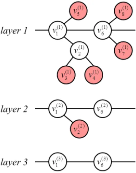
TheLlayer of data can be generated by recursively applying Algorithm 1 forL−1times, which means by taking the output of thelth layer as the input of the(l+ 1)th layer. This process can be illustrated in Figure 2 with L = 3. In this example, the end-nodes are denoted as red. It is to be noted that when moving to higher layers, the number of nodes in each layer decreases with the elimination of the end-nodes. More details are given in the caption of Figure 2.
An illustration of the different G(l) = {V(l), E(l)}, l = 1,2,3 layers constructed from a specific map is given in Figure 3. In the first layer, the nodes are distributed more densely in the map. When approaching higher layers, the tree structure represents more and more abstract information. It is to be noted that the number of the end-nodes (denoted as red asterisks) decreases as the progression of the layers which is a consideration for choosing theL= 3 in our experiments.
3) Data generation: This section describes the details about the construction of the higher-layer range data ri(l+1) and
ˆ
r(l+1)i , where the latter is generated from the former with fixed length. As stated in Algorithm 1, given v(l)i satisfying
Fig. 2. An example of multi-layer GVG: The end-nodes are denoted as red. The red nodesv(1)1 ,v2(1)andv(1)6 in layer 1 are fused with their neighbours respectively, where,v1(2)is composed of(v1(1), v(1)2 , v(1)5 ),v(2)2 is composed of(v1(1), v (1) 2 , v (1) 3 , v (1) 4 )andv (2) 6 is composed of(v (1) 1 , v (1) 6 , v (1) 7 , v (1) 8 ).
Then all the red nodes are eliminated from layer 1. This process will be performed recursively on layer 2 to generate layer 3.
received at the respective nodes are integrated to achieve a better perception.
Given each vi(l) with numel(N(v(l)i )) > 1, firstly a local map is generated using occupancy grid mapping [41] based on the respective range data inlth layer, includingrj(l)carried by
v(l)j ∈N(v(l)i ) andr(l)i . This is achieved by transforming all
rj(l) tori(l)’s coordinate frame, which assumes the knowledge of the global robot poses at all times. In this local map, a virtual scan ri(l+1) is then generated by applying ray casting at position v(l)i with 1◦ angular resolution, which is the same as the setting of the real laser range finder.
As the dimensions of the fused range data ri(l+1) could be different in various nodes, linear interpolation on the data is then performed to keep same dimension of data throughout the process. This leads to an sequencerˆi(l+1)with fixed dimension of 360.
Acknowledging the fact that the interpolated points may not contain high information, a completeness rate, which is the proportion of the laser measured data (dimension of r(l)i
to the whole 360◦ data (dimension ofrˆi(l)) is defined as:
q(l)i = length(r
(l) i )
length(ˆr(l)i ) (1)
wherel= 2· · ·L. This measure is used in the decision making process which is discussed in the next section, thus we denote
qi(1) = 180/360 = 0.5 for uniformity when l = 1. However, the linear interpolation is not applied to layer 1 since the initial laser range data ri(1) always has the same dimension of 180, so that linear interpolation becomes unnecessary. By applying this data pre-processing approach, the laser range data in layer 2 to layer L are kept in the fixed length of 360. Note that it is always r(l)i which is employed to construct the next layer, rather than the pre-processedrˆ(l)i .
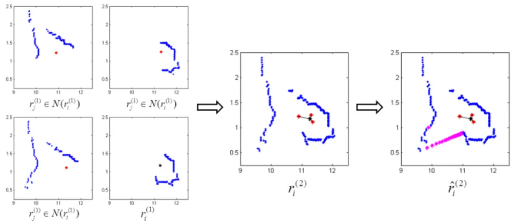
As an example, Figure 4 illustrates the construction of a sequence of input in layer 2 using the corresponding inputs in layer 1, followed by the result after linear interpolation. The details are given in the caption of Figure 4.
B. Decision on Multi-layer Results
1) Construction of the Confidence Tree: With theLlayer of inputs, we can obtain the predicted labels fromLindependent classifiers, which can be formed to be confidence trees withL
layers shown in Figure 5(a), where each node denotes the pre-dicted labelyˆ(l)i ofv(l)i and its corresponding confidencec(l)i
. By maximizing the overall confidence of each tree structure, it is intended to obtain higher accuracy in classification.
All of these tree structures are built from the dependencies in Algorithm 1 except for some minor difference — during the construction of these tree structures, a parent nodev(l+1)i
owns its children vi(l) and vj(l) ∈ M(vi(l)), while the range data of v(l+1)i is constructed from the range data carried by
vi(l) and v(l)j ∈ N(vi(l)). The reason is that for those nodes
vj(l) ∈N(v(l)i ) andv(l)j ∈/ M(v(l)i ), they are also reserved in the higher layer asv(l+1)j and have their own predicted labels, so we don’t consider the influence ofv(l+1)i to them. It is to be noted that the number of such tree structures is equal to the number of nodes left in the layer L, where thevi(L) are the root nodes of these trees.
In our framework, two factors are considered when com-puting the confidencec(l)i , one is the probabilityp(l)i obtained from the classifier for labeling yˆi(l) and the other is the completeness ratioqi(l) obtained from the input sequenceri(l)
which is given in (1). Then the confidencec(l)i is constructed as:
c(l)i =p(l)i ×qi(l) (2)
2) Decision Algorithm: With the confidence trees denoting the predicted label yˆi(l) and its corresponding confidence c(l)i
for each given vi(l), the aim of decision making is then to search the optimized confidencec(l)i∗ and assign the optimized labelyˆ(l)i∗ to each node, leading to the maximum value of the overall confidence.
In each tree structure, we make decisions from children to parents while comparing two consecutive layers based on the decision Algorithm 2. It is to be noted that for the comparison between layer l and layerl−1, the confidence of the parent
vi(l) is always compared to the average optimized confidence of its childrenv(lj−1)and we assume the optimized confidences in layer 1 are known as the original confidences. As for the optimized predicted labels, Algorithm 2 tells that they are only changed to follow their ancestor when this ancestor beats its children in confidence. In other words, if no ancestor of a leaf node gain advantages in confidence, then this leaf node would keep the initial label yˆ(1)i as its optimized label yˆi(1)∗ . Note that although we can obtain the optimized labels for all nodes from this decision algorithm, only the labels of the leaf nodes are exported as output since the classification performance is evaluated based on these leaf nodes. An example is given in Figure 5(b) for better clarity.
(a) Layer 1
(b) Layer 2
(c) Layer 3
Fig. 3. Multi-layer of the GVG graphG(l)={V(l), E(l)}, l= 1,2,3on Fr79. The red nodes correspond to the end-nodes, which will be eliminated in the
next layer, and the black nodes will be preserved. The edges reveals the connection between these nodes.
Fig. 4. An example of constructingri(2)andrˆ(2)i where the axes are in meters. The left four figures illustrater(il)and all of therj(l)carried byv(jl)∈N(vi(l)), where the black asterisk node denotes the position ofvi(l), the red asterisk nodes denote the position ofvj(l)and the blue nodes denote the range data collected from the real environment. Then the middle figure shows the constructedri(2)using ray casting. The interpolated sequence is given on the right, where the magenta points correspond to the interpolated ones. In this example, we haveq(2)i = 332/360 = 0.9222.
Algorithm 2: Decision making on the confidence trees.
Input: Confidence trees where each nodevi(l) denotes the predicted label yˆi(l) and the corresponding confidencec(l)i .
Output: Optimized labels of leaf nodesyˆ(1)i∗ .
1 Initialize c(1)i∗ =c(1)i andyˆi(1)∗ = ˆy(1)i ; 2 for l= 2· · ·L do
3 for vi(l)∈V(l) do
4 Average the optimized confidence of vi(l)’s
childrenv(lj−1) as n1 i P jc (l−1) j∗ ; 5 if 1 ni P jc (l−1) j∗ > c (l) i then 6 Denotec(l)i∗ =n1 i P jc (l−1) j∗ ; 7 else 8 Denotec(l)i∗ =c(l)i ;
9 All descendants ofvi(l) are assigned the label ˆ
yi(l)∗.
10 end
11 end
12 end
We can also evaluate the results obtained from those L
independent classifiers separately with the help of these con-structed trees. To ensure the fairness, results obtained from different layer of classifiers are all compared on the accuracy of bottom layer. Obviously, the results observed from the input of layer 1 do not need to be modified while the higher layers should spread their predicted labels to the bottom layer. Given a specific layerl(l >1), all of the nodes on the bottom layer are assigned the same label as their ancestor in layer l. For example, as shown in Figure 5(b), the v1(l), v(l)2 ,· · ·, v(l)5 will be labeled by thev1(3)’s predicted label when we evaluate the results of layer 3.
IV. SEMI-SUPERVISEDLEARNING ANDCLASSIFICATION
We have introduced the construction of multi-layer inputs and decision making on the multi-layer results in Section III. In this section, we discuss the classification problem of how to train on each layer with the input data and obtain the predicted labels of the testing maps. This is implemented by a deep learning structure, with the capability to automatically learn features from the raw input data. The L layer of inputs are trained through L independent deep learning modes as indicated in Figure 1, though, these models have the same structure with raw laser range data being the input and predicted labels being the output as shown in Figure 6. Thus the discussion below in this section is not confined to any specific layer and hence the superscripts are omitted. It is to be noted that our training process is semi-supervised since both the training map and the testing map are employed for model training, where only the labels of the training map are available. The semi-supervised learning process has the advantage of gaining richer information of data distribution,
(a) Confidence tree
(b) A decision example
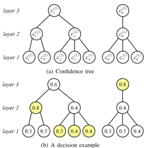
Fig. 5. Confidence trees built from Figure 2 and a corresponding example. (a) The confidence tree: Each parent nodevi(l+1)has childrenvi(l)andvj(l)∈ M(v(il)). (b) The decision example: in this example, let’s assume that the confidence of each node is known. By applying the decision method given in Algorithm 2, firstly we have the initializationc(1)i∗ =c(1)i andyˆ(1)i∗ = ˆ
yi(1). And then average confidence of the children in bottom most layer are compared with their corresponding parents in the immediate upper layer. In the left tree,c(2)1 is larger than the average value ofc(1)1 andc(1)5 , and therefore
c(2)1∗ = 0.8and both the respective children (v(1)1 andv(1)5 ) are assigned the labelyˆ1(2). Thec(2)2 is smaller than the average value ofc(1)2 , c(1)3 andc(1)4 , hence these leaf nodes remain their initial label andc(2)2∗ = (0.5 + 0.4 +
0.4)/3 = 0.4333. Finallyc(3)1 = 0.6is compared with(c(2)1∗ +c
(2) 2∗)/2 =
0.6167. Since the confidence of layer 3 is smaller than the optimized average confidence combined from layer 1 and layer 2, the final optimized confidence isc(3)1∗ = 0.6167and the optimized labels do not change. By applying the same decision process on the right tree in the figure,v(1)6 ,v7(1)andv(1)8 are labeled the same asv(3)6 .
while keeping the spatial consistency as we will introduce in this chapter.
A. Semi-supervised Learning with Graph Regularization
In the classification problem, we denote the training pairs as (Xl ∈ Rm×nl, Y
l ∈ R1×nl) as a convention, where m
denotes the input dimension,nldenotes the number of training samples. Particularly, each column inXlis a sequence of laser range datar, i.e.xil=ri. The testing data can be defined in the same way asXu∈Rm×nu, where n
udenotes the number of testing samples. Then the task of the classification problem is to obtain predicted labels ofXugivenXlandYl. In addition, we denote X = [Xl Xu] ∈ Rm×n as the combination of
training data and testing data with n = nl+nu, since X is fed into the model as a whole during our semi-supervised training process.
As illustrated in Figure 6, the input is firstly fed into a set of fixed parameters (denoted as red) to compute the differences between the consecutive beams in each raw scan, as the consecutive differences can also provide rich information to the place classification and is often employed for extracting geometric features in the previous works [11], [12]. In the practical experiments, we sort both of the input and consecu-tive differences to guarantee the rotational invariance.
Fig. 6. Model training in semi-supervised learning: The second layer has fixed parameters which computes the consecutive differences of our input (denoted as red). Then both the input and the output of the second layer will be fed into the latter process. For the fine-tuning process, theJlabelis imposed to the softmax classifier and all of the parameters in the neural network (except the fixed layer) will be adjusted, whileJgraphis imposed to the last hidden layer and will only influence the feature learning process.
From this point on, both the input and output of this fixed layer are fed into the stacked auto-encoders for feature learn-ing. Auto-encoder is the widely used structure for building deep architectures, which is composed of an encoder and a decoder. By feeding the representation learned from the pre-vious encoder as the input into another auto-encoder, we can obtain the stacked hidden representations as shown in Figure 6. Let’s denote sigmoid function asf(x) = 1/(1 +e−x), then the ith layer of encoder and decoder can be represented as follows:
Hi=f(WiHi−1+bi)
ˆ
Hi−1=f(WiTHi+ci)
(3)
whereHi−1andHˆi−1denote the input and its reconstruction,
Hidenotes the hidden representation andWi, bi, ci denote the weighted parameters respectively1. In this paper, the weights
in each pair of encoder and decoder are tied together as shown in (3).
For each layer of auto-encoder, the unsupervised pre-training is applied to obtain better parameters than random initialization [18] by minimizing the reconstruction cost:
Jpre=
1
mkHi−1−
ˆ
Hi−1k2F (4) Note that the decoder is discarded after pre-training while the encoder is preserved. The hidden representation learned by the last auto-encoder can be regarded as the feature for the input to the classifier.
In the work reported here, the softmax classifier is applied to the features learned from stacked auto-encoders for classi-fication, which is formulated as follow:
pi= exp(wT ih) P jexp(w T jh) (5) 1Wheni=1, H
i−1 is the raw input — the combination of X and its
consecutive differencesXs.
wherepicorresponds to the probability that the hidden repre-sentation vector hbelongs to theith class.
After pre-training and classification, back propagation can be used to fine-tune the whole learning process for further promotion, which means the parameters of preserved encoders and softmax are trained together. In order to keep the local consistency, we add a graph regularization term during tuning to learned representation. The cost function of the fine-tuning is given as follow:
Jf ine=Jlabel+Jgraph
= 1 nl nl X i=1 Jlabel(xil, y i l) + λ n n X i=1 n X j=1 sijkhi−hjk2 (6)
where the first term corresponds to the prediction error of the training data, and the second term is the graph regularization. Here hi andhj are the outputs of the last hidden layer with respect to the inputsxi andxj (xi and xj are two arbitrary columns inX), andsij is the similarity measurement between the samplesxi andxj that are connected in GVG, which is an element of the adjacency graph S = [sij]n×n. Figure 6 also illustrates the way our cost function work. The costs caused by the prediction error is imposed on the softmax classifier and then our graph regularization is imposed on the last hidden layer. Therefore during the fine-tuning theJlabelinfluences all of the parameters, while Jgraph influences parameters except for the softmax classifier.
B. Graph Regularization in Place Classification Problem
As shown in (6), the learned features hi and hj with large weight sij will be pushed together with the graph regularization term. In this section, we describe the details about the construction of the adjacency graphS which can be built in two steps. Firstly we define the connected relationships between samples and then calculate their weights of the connected edges.
In the place classification problem, the connected relation-ships in the topological graph GVG are directly employed to the adjacency graph. Then the samples with close coordinates are forced to be represented by the features with close dis-tances. As for the weights which corresponds to the strength of the graph regularization, it is inversely associated with two distances, i.e. the distance between coordinates and the distance between the input data, which can be formulated as:
sij= α dij + β kxi−xjk2 (7)
whereαandβ are constant weights,dijdenotes the Euclidean distance between the sample coordinates. The second term defines the Euclidean distance between the input data. This weighting scheme dose not only evaluate the geometrical information, but also considers the closeness between inputs. For example, given an edge that connects two nodes belonging to corridor and office respectively, although dij is small, kxi−xjk2 can be large. Therefore, these two nodes are not forced to be too close in the representation space and the discriminative information could be preserved.
V. EXPERIMENTS
To validate the effectiveness of our end-to-end multi-layer learning system, we conduct experiments on six data sets collected from six international university indoor environments using (including the Centre for Autonomous Systems at the University of Technology, Sydney, several buildings in the University of Freiburg, the German Research Centre for Artifi-cial Intelligence in Saarbruecken, and the Intel Lab in Seattle). On each real grid map, a simulated robot collected laser range data using a virtual on-board 2D laser range finder (with a maximum range of 30m and a horizontal field of view of 180◦) at the previous mentioned GVG nodes.
It is to be noted that the classes defined by humans can be somewhat vague and plentiful according to the different functions of places. However, the 2D range data do not contain enough discriminative information to classify all these human-designed classes. Therefore, we consider 3 target classes as: Class 1-space designed for a small number of individuals including cubicle, office, printer room, kitchen, bathroom, stairwell and elevator; Class 2-space for group activities in-cluding meeting room and laboratory; Class 3-corridor.
Among these six data sets, two of them (Fr79 and Intellab) contain all of the 3 classes but the others contain only parts of these classes. We conduct leave-many-out training, which means one data set is utilized for training and others are used for testing. Therefore, we obtained two groups of results by training on Fr79 and Intellab respectively.
For parameter setting, we choose L = 3 based on the difference between two consecutive layers, which is measured by distance between their mean completeness rates. The mean completeness of layer l is given as follow:
q(l)=X
i
qi(l) (8)
where qi(l) is the completeness rate of node i in layer l as defined in (1). If the distance between q(l) andq(l+1) is tiny, then for a node existing in both layer, its corresponding laser measured data in these two layers are very close. Consequent-ly, the slightly difference leads to tiny change in the predicting results and thus it is meaningless to consider the higher layer
l+ 1. Taking the map Fr79 as an example, it hasq(1)= 0.50,
q(2) = 0.91,q(3) = 0.98 andq¯(4) = 0.99. Sinceq(4) is very close to q(3), we choose L= 3 in this paper. For dimension configuration of the deep architecture in Figure 6, we set the dimension of each layer asm−m−100−24−3 given the input X ∈Rm×n. The input and the consecutive differences
layer both have the same dimension as the raw inputm, where
m = 180 for L = 1 and m = 360 for L = 2,3. For the following hidden layers, we set the dimension of the hidden representationH1as 100 based on experience. The dimension of the hidden representation H2 is set to be 24, which is the same as the dimension of the handcrafted features in [8] for fair comparison. Finally the output of our model represents a probabilistic measure of data belonging to each class. Thus the output dimension is the same as the number of our classes.
TABLE I
MULTI-LAYER RESULTS TRAINED ONINTELLAB.
Map L1(%) L2(%) L3(%) UTS 85.20 89.49 91.24 SarrB 86.55 87.64 91.32 FrUA 86.23 92.96 91.69 FrUB 90.29 98.87 99.84 Fr79 81.99 85.87 87.90 Average 86.05 90.97 92.40 TABLE II
MULTI-LAYER RESULTS TRAINED ONFR79.
Map L1(%) L2(%) L3(%) UTS 81.70 85.99 89.93 SarrB 84.16 95.44 90.46 FrUA 90.43 94.70 96.91 FrUB 88.67 98.87 99.51 Intellab 72.55 79.81 82.73 Average 83.50 90.96 91.91
A. Multi-layer Results without Graph Regularization
We first conduct experiments to evaluate the performance of our multi-layer inputs. Table I and Table II shows the leave-many-out classification results training on Intellab and Fr79 respectively. It is to be noted that the graph regularization is not considered here and therefore,λ= 0 in the cost function (6). In general, results of higher layers are better than that of lower layers due to the richer information contained in each node on the higher layers.
B. Multi-layer Results with Graph Regularization
We also carried out experiments to validate the effectiveness of the graph regularization. The algorithm remains the same as previous settings, however, we changed the value ofλ= 1
to add the graph regularization. In this experiments, we pay more attention to the geometrical neighborhood, thus we use
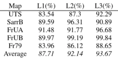
α = 2/3 and β = 1/3 in (7) for the construction of the adjacency graph. The classification results are shown in Table III and Table IV, which are trained on Intellab and Fr79 respectively. The results have the similar trends as in Table I and Table II, where higher layers give rise to better accuracies. Further comparisons of Table I and Table III show that the feature learning with graph regularization performs better than without it. It reveals that the graph regularization has the advantage of improving classification performances by keeping the local consistency.
C. Fusion Results
Finally, we show the accuracies of the multi-layer graph regularized method with fusion in Table V and Table VI. When compared with the results of each single layer as shown in Table III and Table IV, the fusion results achieved better accu-racies. For the results trained on Intellab, the average accuracy of fusion results risen to 94.02%fromL1:87.71%,L2:92.14%
andL3:92.66%, and the results trained on Fr79 also reached
TABLE III
MULTI-LAYER RESULTS TRAINED ONINTELLAB WITH GRAPH REGULARIZATION. Map L1(%) L2(%) L3(%) UTS 83.54 87.3 92.29 SarrB 89.59 96.31 90.89 FrUA 91.48 91.77 96.68 FrUB 89.97 99.19 99.84 Fr79 83.96 86.12 88.65 Average 87.71 92.14 93.67 TABLE IV
MULTI-LAYER RESULTS TRAINED ONFR79WITH GRAPH REGULARIZATION. Map L1(%) L2(%) L3(%) UTS 80.47 89.23 90.02 SarrB 87.20 96.75 95.23 FrUA 91.06 96.12 97.47 FrUB 89.48 98.87 99.51 Intellab 73.00 79.89 82.51 Average 84.24 92.17 92.95
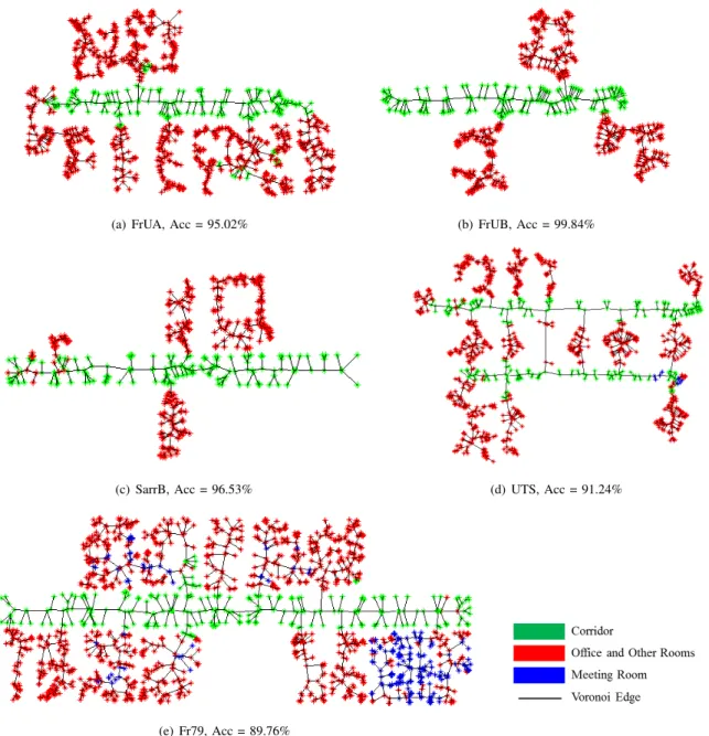
fused test results trained on Intellab are diagrammatically illustrated in Figure 7. It is to be noted that confusions between Class 1 (office room and other rooms) and Class 2 (meeting room) account for the major misclassifications especially in the test map of Fr79. The cause might be that Class 1 is featured with narrow environment including massive clutters while the Class 2 is featured with relatively larger spaces, therefore the corners of meeting room are mostly classified as office room and other rooms and some center positions of office room are assigned as office room.
Through the experiments above, one can see that our framework is beneficial from these two aspects:
1) By regularizing the deep architecture with the adjacency graph, the learned features are expected to be learned with spatial invariance intrinsically, while the hand-crafted features not able to encoding the relationship between neighboring n-odes. The automatic feature learning also simplifies the feature engineering significantly, enabling the end-to-end learning.
2) The better discriminative performance is achieved by fusion on the confidence tree, which comprehensively consid-ers the results from different layconsid-ers. The information can be insufficient in lower layer due to narrow FOV. In addition, in higher layers, as the FOV may cover more than one place, the multiple labels may confuse the classifier. The tree decision avoids the two problems to some extent.
D. Algorithm Comparison
To further validate the effectiveness of the proposed algo-rithm, it is compared to one baseline method as well as three state-of-the-art methods, including:
• SVMThe support vector machine (SVM) is employed as a baseline classifier. It is based on 24-dimensional hand-engineered features as implemented in [8]. Specifically, 21 features are constructed based on statistical and geo-metrical information from the180◦ FOV raw range data,
which is a subset of the features used in [11]. The other 3 features are constructed to describe the time domain information follow [42].
• SPCoGVG Semi-supervised place classification over a
generalized Voronoi graph (SPCoGVG) [8], which is composed of SVM and conditional random field (CRF) to ensure the generalization ability. It also uses the 24-dimensional hand-engineered feature the same as the SVM.
• LVQ Mar.This method uses Learning Vector Quantiza-tion (LVQ) for classificaQuantiza-tion and Markov Model to incor-porate the past inference [33]. Similar to our work, they take raw laser scans as input, while their input can only be calibrated360◦FOV range data. LVQ can be regarded
as a shallow neural network with one hidden layer, thus the dimension of the hidden layer is set to be 24, which is the same as the dimension as SVM, SPCoGVG and our method. To build the time sequence, we generate a moving trajectory based on our GVG nodes, on which the Markov Model is applied. We reimplement their method follow their paper for comparison.
• DBMM Dynamic Bayesian Mixture Models (DBM-M) [17] is a method that combines two SVM classifiers using a mixture of probabilistic models, and incorporates past inferences using a dynamic Bayesian process. It is also based on hand-engineered features constructed follow [11], while a larger subset with 50 dimensions is considered in this work. The features are extracted from both 180◦ FOV and360◦ FOV laser scan data for
comparison. A time sequence is also required to build the dynamic Bayesian network, which is the constructed the same as the moving trajectory in the LVQ Mar. We reim-plement their method follow their paper for comparison. We also reimplement this method by ourselves.
As can be seen from Table V and Table VI, our method achieves superior results compared to the others. Specifically, 1) Our method and LVQ Mar. both employ the raw data to learn the features. However, LVQ Mar. is not comparable to SVM while ours outperforms SVM considerably. Particularly, LVQ performs poor when trained on FR79 and tested on Intellab as shown in Table VI. A main reason is that the structure of Class 1 (corridors) at Intellab is slightly different than that of the other maps, and LVQ is not able to capture the variance with its features learned from the shallow ar-chitecture. As a result, the average performance of LVQ is even poorer when trained on Intellab and tested on the others maps in Table V. The result indicates that our method learns more generalizable features by owning the deep architecture and considering the spatial consistency. With the shallow architecture, LVQ Mar. cannot generate a good performance even it models the temporal information (spatial consistency in moving direction).
2) DBMM is expected to outperform SVM as it fuses two SVMs with different set of hand-crafted features. Though it outperforms SVM in Table VI, the DBMM with 180◦ FOV achieves low accuracy on SarrB in Table V. In this case, one of the SVMs has severe misclassification between the Class 1 and Class 2 with only accuracy at 77.87%. Even with the
other SVM having accuracy at85.03%, the combined accuracy with consideration of temporal information only achieves
79.83%. This result indicates the hand-crafted features should be carefully chosen, while their robustness to different maps is not guaranteed. It is also worth to mention that DMBB with 180◦ FOV outperforms the DBMM with 360◦ FOV in Table VI, especially on the test SarrB, while in Table V the DBMM with 360◦ FOV generally performs better. This fact reflects that only considering the sensor information in one resolution can be insufficient to make a comprehensive classification.
3) Another possible reason that our method and SPCoGVG outperform LVQ Mar. and DBMM is that, the completed spatial consistency modeling by the adjacency graph can better constrain the classifier than the temporal consistency modeling by moving trajectory. For example, when the robot moves from Class 1 to Class 2, LVQ Mar. and DBMM only consider the past inferences of the nodes with Class 1, while our method and SPCoGVG additionally take the inference of consequent nodes with Class 2 into consideration. Besides, our method is slightly better than SPCoGVG, indicating that considering the constraints, e.g. spatial consistency, in feature learning step may be better than in classification step, as the former occurred in nonlinear feature space, while the latter utilizes the simple weighted sum.
In summary, the proposed method achieves state-of-art per-formance by using the spatial proximity aided feature learning and confidence tree based multi-layer fusion, without referring to the hand-crafted feature engineering. Besides, we think a more valuable insight is that the practice with architecture of hierarchical feature learning and decision, which can simply incorporate the prior knowledge at the same time, can be leveraged to in other tasks, especially the robot cognitive and decision tasks, as they have many structured or hierarchical priors.
VI. CONCLUSIONS
In this paper, we presented an end-to-end place classification framework. We implemented a multi-layer learning frame-work, including the construction of multi-layer inputs and de-cision making on the multi-layer results. Each layer of inputs were fed into a semi-supervised model for feature learning and classification, which guaranteed the local consistency with a graph regularization.
Experimental results showed that the higher layer input data led to higher classification accuracy, which validated the effectiveness of the multi-layer structure. By performing the semi-supervised learning with or without graph regu-larization, we also showed that graph regularization helps promoting the classification performance by incorporating the local consistency. Furthermore, the fusion results based on the confidence tree achieved comparable results to the state-of-the-art method. In a nutshell, we achieved the generalization ability and preserved the local consistency in our end-to-end place classification framework. Future work is to apply our framework on other type of sensor data, such as RGB-D data, which have more representative and discriminative ability.
REFERENCES
[1] L. Yuan, K. C. Chan, and C. G. Lee, “Robust semantic place recognition with vocabulary tree and landmark detection,” in Proc. IROS 2011 workshop on Active Semantic Perception and Object Search in the Real, World, 2011.
[2] A. Pronobis and P. Jensfelt, “Hierarchical multi-modal place categoriza-tion.” inECMR, 2011, pp. 159–164.
[3] A. Ranganathan and J. Lim, “Visual place categorization in maps,” in
Intelligent Robots and Systems (IROS), 2011 IEEE/RSJ International Conference on. IEEE, 2011, pp. 3982–3989.
[4] A. Poncela, C. Urdiales, B. Fern´andez-Espejo, and F. Sandoval, “Place characterization for navigation via behaviour merging for an autonomous mobile robot,” inElectrotechnical Conference, 2008. MELECON 2008. The 14th IEEE Mediterranean. IEEE, 2008, pp. 350–355.
[5] C. Galindo, J.-A. Fern´andez-Madrigal, J. Gonz´alez, and A. Saffiotti, “Robot task planning using semantic maps,”Robotics and Autonomous Systems, vol. 56, no. 11, pp. 955–966, 2008.
[6] H. Celikkanat, G. Orhan, N. Pugeault, F. Guerin, E. Sahin, and S. Kalkan, “Learning context on a humanoid robot using incremental latent dirichlet allocation,” Autonomous Mental Development, IEEE Transactions on, vol. PP, no. 99, pp. 1–1, 2015.
[7] A. Aydemir, K. Sjoo, J. Folkesson, A. Pronobis, and P. Jensfelt, “Search in the real world: Active visual object search based on spatial relations,” inRobotics and Automation (ICRA), 2011 IEEE International Conference on. IEEE, 2011, pp. 2818–2824.
[8] L. Shi and S. Kodagoda, “Towards generalization of semi-supervised place classification over generalized voronoi graph,”Robotics and Au-tonomous Systems, vol. 61, no. 8, pp. 785–796, 2013.
[9] N. S¨underhauf, F. Dayoub, S. McMahon, B. Talbot, R. Schulz, P. Corke, G. Wyeth, B. Upcroft, and M. Milford, “Place categorization and semantic mapping on a mobile robot,”arXiv preprint arXiv:1507.02428, 2015.
[10] Y. Liao, S. Kodagoda, Y. Wang, L. Shi, and Y. Liu, “Understand scene categories by objects: A semantic regularized scene classifier using convolutional neural networks,”arXiv preprint arXiv:1509.06470, 2015. [11] O. M. Mozos, C. Stachniss, and W. Burgard, “Supervised learning of places from range data using adaboost,” inRobotics and Automation, 2005. ICRA 2005. Proceedings of the 2005 IEEE International Confer-ence on. IEEE, 2005, pp. 1730–1735.
[12] P. Sousa, R. Ara´ujo, and U. Nunes, “Real-time labeling of places using support vector machines,” in Industrial Electronics, 2007. ISIE 2007. IEEE International Symposium on. IEEE, 2007, pp. 2022–2027. [13] H. Choset and J. Burdick, “Sensor based planning. I. the generalized
voronoi graph,” inRobotics and Automation, 1995. Proceedings., 1995 IEEE International Conference on, vol. 2. IEEE, 1995, pp. 1649–1655. [14] W. Shi and J. Samarabandu, “Investigating the performance of corridor and door detection algorithms in different environments,” inInformation and Automation, 2006. ICIA 2006. International Conference on. IEEE, 2006, pp. 206–211.
[15] L. Shi, S. Kodagoda, and G. Dissanayake, “Laser range data based semantic labeling of places,” inIntelligent Robots and Systems (IROS), 2010 IEEE/RSJ International Conference on. IEEE, 2010, pp. 5941– 5946.
[16] L. Shi, S. Kodagoda, and G. Dissanayake, “Multi-class classification for semantic labeling of places,” inControl Automation Robotics & Vision (ICARCV), 2010 11th International Conference on. IEEE, 2010, pp. 2307–2312.
[17] C. Premebida, D. R. Faria, F. A. Souza, and U. Nunes, “Applying probabilistic mixture models to semantic place classification in mobile robotics,” in Intelligent Robots and Systems (IROS), 2015 IEEE/RSJ International Conference on. IEEE, 2015, pp. 4265–4270.
[18] G. Hinton and R. Salakhutdinov, “Reducing the dimensionality of data with neural networks,”Science, vol. 313, no. 5786, pp. 504 – 507, 2006. [19] G. Hinton, S. Osindero, and Y. Teh, “A fast learning algorithm for deep
belief nets,”Neural computation, 2006.
[20] Y. LeCun, Y. Bengio, and G. Hinton, “Deep learning,”Nature, vol. 521, no. 7553, pp. 436–444, 2015.
[21] A. Krizhevsky, I. Sutskever, and G. E. Hinton, “Imagenet classification with deep convolutional neural networks,” inAdvances in neural infor-mation processing systems, 2012, pp. 1097–1105.
[22] R. Girshick, “Fast r-cnn,” in Proceedings of the IEEE International Conference on Computer Vision, 2015, pp. 1440–1448.
[23] R. Collobert, J. Weston, L. Bottou, M. Karlen, K. Kavukcuoglu, and P. Kuksa, “Natural language processing (almost) from scratch,” The Journal of Machine Learning Research, vol. 12, pp. 2493–2537, 2011.
TABLE V
GRAPH REGULARIZED FUSION RESULTS TRAINED ONINTELLAB AND RESULTS USINGSPCOGVG.
Map Multi-layer fusion(%) SVM(%) SPCoGVG(%) LVQ Mar.(%) DBMM180◦(%) DBMM360◦(%) UTS 91.24 87.74 90.72 82.75 88.88 88.70 SarrB 96.53 85.68 88.72 75.49 79.83 86.77 FrUA 95.02 96.04 96.52 89.95 94.38 95.89 FrUB 99.84 97.25 98.71 83.33 95.96 97.41 Fr79 89.76 88.34 92.04 77.85 89.88 93.28 Average 94.48 91.01 93.39 81.87 89.79 92.41 TABLE VI
GRAPH REGULARIZED FUSION RESULTS TRAINED ONFR79AND RESULTS USINGSPCOGVG.
Map Multi-layer fusion(%) SVM(%) SPCoGVG(%) LVQ Mar.(%) DBMM180◦(%) DBMM360◦(%)
UTS 90.54 83.54 89.84 88.97 87.22 85.46 SarrB 98.27 82.43 93.71 92.84 91.97 86.99 FrUA 97.23 92.72 97.71 96.12 95.97 96.84 FrUB 99.51 80.74 99.19 97.89 96.93 97.09 Intellab 82.40 79.89 86.89 57.19 83.22 85.36 Average 93.59 83.86 93.47 86.60 91.06 90.35
[24] I. Sutskever, O. Vinyals, and Q. V. Le, “Sequence to sequence learning with neural networks,” inAdvances in neural information processing systems, 2014, pp. 3104–3112.
[25] G. E. Dahl, D. Yu, L. Deng, and A. Acero, “Context-dependent pre-trained deep neural networks for large-vocabulary speech recognition,”
Audio, Speech, and Language Processing, IEEE Transactions on, vol. 20, no. 1, pp. 30–42, 2012.
[26] W.-L. Zheng and B.-L. Lu, “Investigating critical frequency bands and channels for eeg-based emotion recognition with deep neural networks,”
Autonomous Mental Development, IEEE Transactions on, vol. 7, no. 3, pp. 162–175, Sept 2015.
[27] S. Rifai, P. Vincent, X. Muller, X. Glorot, and Y. Bengio, “Contractive Auto-Encoders: Explicit invariance during feature extraction,” inICML, 2011.
[28] S. Rifai, G. Mesnil, P. Vincent, X. Muller, Y. Bengio, Y. Dauphin, and X. Glorot, “Higher order contractive auto-encoder,” inProceedings of the 2011 European conference on Machine learning and knowledge discovery in databases - Volume Part II, ser. ECML PKDD’11. Berlin, Heidelberg: Springer-Verlag, 2011, pp. 645–660.
[29] P. Vincent, “A connection between score matching and denoising au-toencoders,”Neural Comput., vol. 23, no. 7, pp. 1661–1674, Jul. 2011. [30] R. Hadsell, A. Erkan, P. Sermanet, M. Scoffier, U. Muller, and Y. LeCun, “Deep belief net learning in a long-range vision system for autonomous off-road driving,” inIntelligent Robots and Systems, 2008. IROS 2008. IEEE/RSJ International Conference on. IEEE, 2008, pp. 628–633. [31] I. Lenz, H. Lee, and A. Saxena, “Deep learning for detecting robotic
grasps,”The International Journal of Robotics Research, vol. 34, no. 4-5, pp. 705–724, 2015.
[32] O. Sigaud and A. Droniou, “Towards deep developmental learning,” Au-tonomous Mental Development, IEEE Transactions on, vol. PP, no. 99, pp. 1–1, 2015.
[33] B. Kaleci, C. M. Senler, H. Dutagaci, and O. Parlaktuna, “A proba-bilistic approach for semantic classification using laser range data in indoor environments,” inAdvanced Robotics (ICAR), 2015 International Conference on. IEEE, 2015, pp. 375–381.
[34] A. Pronobis and P. Jensfelt, “Large-scale semantic mapping and reason-ing with heterogeneous modalities,” inRobotics and Automation (ICRA), 2012 IEEE International Conference on. IEEE, 2012, pp. 3515–3522. [35] O. Martinez Mozos, R. Triebel, P. Jensfelt, A. Rottmann, and W. Bur-gard, “Supervised semantic labeling of places using information extract-ed from sensor data,”Robotics and Autonomous Systems, vol. 55, no. 5, pp. 391–402, 2007.
[36] A. Ranganathan, “Pliss: Detecting and labeling places using online change-point detection.” inRobotics: Science and Systems, 2010. [37] R. Hadsell, S. Chopra, and Y. LeCun, “Dimensionality reduction by
learning an invariant mapping,” inProceedings of the 2006 IEEE Com-puter Society Conference on ComCom-puter Vision and Pattern Recognition - Volume 2, ser. CVPR ’06. Washington, DC, USA: IEEE Computer Society, 2006, pp. 1735–1742.
[38] J. Weston, F. Ratle, H. Mobahi, and R. Collobert, “Deep learning via semi-supervised embedding,” inNeural Networks: Tricks of the Trade. Springer, 2012, pp. 639–655.
[39] R. Hadsell, S. Chopra, and Y. LeCun, “Dimensionality reduction by learning an invariant mapping,” inComputer vision and pattern recog-nition, 2006 IEEE computer society conference on, vol. 2. IEEE, 2006, pp. 1735–1742.
[40] T. Tao, S. Tully, G. Kantor, and H. Choset, “Incremental construction of the saturated-gvg for multi-hypothesis topological slam,” inRobotics and Automation (ICRA), 2011 IEEE International Conference on. IEEE, 2011, pp. 3072–3077.
[41] S. Thrun, W. Burgard, and D. Fox,Probabilistic robotics. MIT press, 2005.
[42] B. Hjorth, “Eeg analysis based on time domain properties,” Electroen-cephalography and clinical neurophysiology, vol. 29, no. 3, pp. 306–310, 1970.
(a) FrUA, Acc = 95.02% (b) FrUB, Acc = 99.84%
(c) SarrB, Acc = 96.53% (d) UTS, Acc = 91.24%
(e) Fr79, Acc = 89.76%